*
Corresponding author:
E-mail: [email protected]
Received: July 10, 2017
Approved: August 8, 2017
How to cite: Farias PS, Souza LS, Paiva AQ, Oliveira AS, Souza LD, Ledo CAS. Hourly, daily, and monthly soil temperature fluctuations in a drought tolerant crop. Rev Bras Cienc Solo. 2018;42:e0170221.
https://doi.org/10.1590/18069657rbcs20170221
Copyright: This is an open-access article distributed under the terms of the Creative Commons Attribution License, which permits unrestricted use, distribution, and reproduction in any medium, provided that the original author and source are credited.
Division - Soil Processes and Properties | Commission - Soil Physics
Hourly, Daily, and Monthly Soil
Temperature Fluctuations in a
Drought Tolerant Crop
Polianna dos Santos de Farias(1)*
, Luciano da Silva Souza(2)
, Arlicélio de Queiroz Paiva(3) , Áureo Silva de Oliveira(2)
, Laércio Duarte Souza(4)
and Carlos Alberto da Silva Ledo(4)
(1)
Universidade Federal do Recôncavo da Bahia, Programa de Pós-Graduação em Solos e Qualidade de Ecossistemas, Cruz das Almas, Bahia, Brasil.
(2)
Universidade Federal do Recôncavo da Bahia, Centro de Ciências Agrárias, Ambientais e Biológicas, Cruz das Almas, Bahia, Brasil.
(3)
Universidade Estadual de Santa Cruz, Departamento de Ciências Agrárias e Ambientais,
Campus Soane Nazaré de Andrade, Ilhéus, Bahia, Brasil.
(4)
Empresa Brasileira de Pesquisa Agropecuária, Embrapa Mandioca e Fruticultura, Cruz das Almas, Bahia, Brasil.
ABSTRACT: Soil temperature is a physical property of great agricultural importance in the soil-plant relationship and in energy exchange with the atmosphere. This study was conducted in a degraded Cambissolo Háplico Ta Eutrófico (Cambisol; Inceptisol) in the Irecê Identity Territory, Bahia, Brazil, aiming to evaluate the hourly, daily, and monthly fluctuations of soil temperature at depth, and soil thermal diffusivity in the castor bean crop. Hourly soil temperature data from February 4, 2014, to September 30, 2015, were obtained by using thermocouple sensors (copper-constantan) horizontally installed at 0.05, 0.10, and 0.20 m depths. Soil thermal diffusivity was estimated by phase and amplitude methods. Results showed that, for most days, the soil temperature was at the level recommended for castor bean. The maximum and minimum hourly and daily soil temperatures were observed in October and July, respectively, and the maximum soil temperature values occurred at 4 p.m. (0.05 m), 5 p.m. (0.10 m), and 7 p.m. (0.20 m). Soil temperature variability is low, requiring few measurement points to estimate this factor in an area. The amplitude method led to soil thermal diffusivity values compatible with results in the literature. The absence of a relationship between thermal diffusivity and soil moisture was attributed to the clay-loam soil texture, predominance of micropores, and iron oxides allowing greater approximation to the soil particles, with high thermal diffusivity even under low soil moisture conditions.
INTRODUCTION
From the agronomic point of view, castor bean is very drought tolerant, producing satisfactorily under low rainfall conditions. This crop has a high need for solar radiation, preferably long periods of daylight, air temperature around 28 °C (Beltrão et al., 2007), and soil temperature around 29 °C, so the seedling can emerge more quickly (Lucena et al., 2014). The Brazilian semiarid region provides good conditions for adaptation of castor bean (Cartaxo et al., 2004) and the region is considered to have potential for biodiesel production in the Brazilian Northeast (Brasil, 2011).
High natural soil fertility found in the Irecê Identity Territory (Silva et al., 1993) contributed to this region becoming the highest dry edible bean, corn, and castor bean producer in the state of Bahia and the Brazilian Northeast region in the past (Sei, 2003). Intense reduction in the natural Caatinga vegetation and substitution by rainfed and irrigated agriculture, with intensive use of agricultural mechanization, occurred in this region from 1980 to 2007 (Paiva et al., 2015). These changes degraded the soil and altered the hydrological cycle, especially concerning increased irregularity of rainfall. Consequently, bean and corn crop production declined, and castor bean became the agricultural support crop for the region. Castor bean production is concentrated in the 19 municipalities that compose the Irecê Identity Territory, which represents approximately 80 % (76 thousand tons) of all castor bean production in Brazil (Queiroga et al., 2011). This crop is traditionally produced on small and medium-sized farms and has significant social value through creation of employment and income opportunities in rural areas (Ribeiro et al., 2009). However, castor bean crop area has been declining in recent years, decreasing 63 % from 2015 to 2016 (Brasil, 2017), mainly due to increasing irregularity of water availability, which is worsened by minimal plant cover and high soil compaction from excessive use of heavy duty harrowing equipment.
Soil temperature directly affects plant growth and development, and indirectly affects evapotranspiration; these conditions are even more relevant in semi-arid environments, where both factors (temperature and soil water) are critical. The soil not only stores water, solutes, and gases and allows transfer procedures, but also stores and transmits heat, which intervenes in all biological, physical, and chemical processes (Prevedello, 2010). For that reason, and the fact that each soil type has its own properties, it is necessary to identify the thermal properties for each situation (Rao et al., 2005; Danelichen and Biudes, 2011).
Several studies have been performed to evaluate daily (Kunz et al., 2002; Oliveira et al., 2010; Belan et al., 2013; Diniz et al., 2013a, 2014), monthly (Diniz et al., 2013a), and yearly (Carneiro et al., 2014) soil temperature fluctuations. The correlation between soil and air temperatures was studied by Azevedo and Galvani (2003), Carvalho et al. (2009), Belan et al. (2013), and Awe et al. (2015), while thermal diffusivity in soil was evaluated by Amaro Filho et al. (2008), Diniz et al. (2014), Soares et al. (2014), and Oliveira et al. (2015). Several studies conducted in different soil management systems obtained a significant and inverse relationship between soil temperature and cover crop with residual or cultural biomass (Dourado-Neto et al., 1999; Silva et al., 2006).
Soil temperature is important for plant growth and development, especially because of its effect on evapotranspiration. Considering the increasing scarcity of soil water in the Irecê Identity Territory and the lack of specific data for this region, detailing soil thermal properties can contribute to guiding farm management practices with the aim of more successful cultivation of castor bean in that territory. This may assist in maintaining or increasing crop area and crop yield.
MATERIALS AND METHODS
This study was performed on a farm in the municipality of São Gabriel (11° 13’ 45” S; 41° 54’ 43” W) in Bahia, Brazil. The climate, according to the Köppen classification system, is semiarid (BS), with mean annual rainfall of 650 mm, and mean annual temperature of
23.5 °C. The soil is classified as a Cambissolo Háplico Ta Eutrófico (Santos et al., 2013),
which corresponds to Cambisol (WRB, 2014) or Inceptisol (Soil Survey Staff, 2014). The castor bean ‘BRS-149 Nordestina’ was used, at a 3.0 × 1.0 m spacing. The study included two crop seasons: 2013/2014 and 2014/2015. Disturbed and undisturbed samples were taken at six points in the experimental area, at 0.00-0.10, 0.10-0.20, and 0.20-0.40 m depths, for soil analysis.
Particle size analysis was performed by the pipette method (Gee and Or, 2002), using 1 mol L-1 sodium hexametaphosphate for dispersion and a Wiegner mechanical shaker at 50 rpm for 16 hours. The sand fraction after drying was fractionated into five classes: very coarse sand (1-2 mm), coarse sand (0.5-1 mm), medium sand (0.25-0.5 mm), fine sand (0.10-0.25-mm), and very fine sand (<0.10 mm) using a set of sieves coupled to an electromagnetic stirrer for 3 min. Soil bulk density (BD) was determined by the volumetric ring method (Grossman and Reinsch, 2002), obtained by the following expression: BD (Mg m-3) = soil dry matter weight/soil volume of 310 cm3. Macroporosity and microporosity
(m3 m-3) were obtained by subjecting the undisturbed and saturated samples to -6 kPa
potential using a tension table (Oliveira, 1968). Total porosity (TP) was calculated by the sum of the macroporosity and microporosity.
Soil temperature was monitored at 12 points in the experimental area, spaced at 0, 45, 75, and 120 m on the X coordinate, and 0, 45, and 90 m on the Y coordinate, covering an area of 10,800 m2. Mini-soil sample pits were opened at each measurement point, and three thermocouple sensors (copper-constantan) were installed horizontally at 0.05, 0.10, and 0.20 m depths and linked to a datalogger device, scheduled to perform hourly readings and store the data. In this study, data recorded from February 4, 2014, to September 30, 2015, were analyzed by obtaining the mean for hourly, daily, and monthly data from January to December. Considering the evaluation period, data from a single year was considering for January, November, and December, and data from a mean of two years for other months.
Soil temperature values were initially analyzed by using descriptive statistics, considering the mean, amplitude, and coefficient of variation (CV); and data normality was evaluated by the Shapiro-Wilk test (p<0.05). The CV values were classified as low variability (≤10 %), mean variability (10 to 20 %), high variability (20 to 30 %), and very high variability (>30 %) (Pimentel-Gomes and Garcia, 2002). Hourly and daily means by depth and for each month were compared by the Tukey test (p<0.05).
The hourly and daily data were then subjected to analysis of variance in a split-plot design, considering the month as the main plot, the hour or day as the split-plot, and depth as the split-split-plot, with the replications consisting of the 12 points in the experimental area in which thermocouples were installed. The definition of this statistical analysis model was based on the study of Ferreira et al. (2012), which proposed statistical procedures in experimental designs with restricted randomization. The hourly and daily mean data were compared by the Scott-Knott test (p<0.05).
The number of measurement points required to estimate the soil temperature in an area was calculated by the formula n = (tα × CV/D)2, in which n is the minimum number of
measurement points, tα is the value of Student’s t-test for α probability level, CV is the coefficient of variation (%), and D is the difference from the mean (%) by using 5, 10, 15, 20, 25, and 30 % (Cline, 1944).
in the meteorological station in the experimental area. The performance of the adjusted equations was evaluated using the air and soil temperature data at the depth of 0.05 m for July (lowest annual monthly soil temperature), September (highest annual monthly soil temperature), and December (mean annual monthly soil temperature) in 2016 months, not used to equations adjust. The statistical performance of the adjusted equations was evaluated by the indices calculated based on equations 1, 2, and 3:
(Oi - Ei)2 1 n
i = 1 n
RMSE= Eq. 1
(
)
+ +=
= =
2 _ _
1 2
1
/
1 E O E O O O
d i i
n
i i i n
i
Eq. 2
C = r × D Eq. 3
in which RMSE = root-mean-square error, the closer to 0, the better (Willmott, 1981); d = concordance index of Willmott (1981), which ranges from 0 (no agreement) to 1 (perfect agreement); C = performance index of Camargo and Sentelhas (1997), classified as optimal (>0.85), very good (0.76-0.85), good (0.66-0.75), medium (0.61-0.65), tolerable (0.51-0.60), poor
(0.41-0.50), and very poor (≤0.40); n = number of data; Oi = observed value; Ei = estimated
value; Ō = mean of observed values; and r = Pearson’s correlation coefficient.
Soil thermal diffusivity was calculated by using soil temperature values recorded every hour, from 12 midnight to 11 p.m., at the 0.05 and 0.20 m depths. Diffusivity means were calculated for each month, as well as the means for the eight months with soil moisture values that were the highest (March, April, May, and November 2014; and January, February, March, and May 2015), medium (March, April, June, and December 2014; and January, March, April, and June 2015), and lowest (April, September, November, and December 2014; and February, March, May, and September 2015). Values for each month or for eight months were related to respective mean soil moisture. Amplitude and phase methods were utilized to determine soil thermal diffusivity (Reichardt and Timm, 2012). Soil thermal diffusivity (D) at different depths by the amplitude method was determined by the equation 4:
D = ω ✕
2
(z2 - z1)
Ɩn A1 A2
2
in which A1 and A2 are the temperature wave amplitudes (difference among the maximum
and the minimum temperature of the day) at depths z1 (0.05 m) and z2 (0.20 m), respectively; and ω = 2π/p, where p is the time required to complete a wave cycle. Soil thermal diffusivity (D) by the phase method was obtained by the equation 5:
D =
1
✕
2ω
(z
2- z
1)
Δt
2
in which ω = 2π/p, where p is the time required to complete a wave cycle, z1 and z2
are soil depths (0.05 and 0.20 m, respectively), and Δt = t2 - t1, Δt is the time interval
between t1 and t2, which are the times when the maximum temperature waves reach
the depths of z1 and z2.
Data were substituted in the above equations, resulting in soil thermal diffusivity (D) for the two methods, in m2 s-1.
Soil moisture was monitored at the same 12 points where soil temperature was recorded by using Campbell CS616-L150 sensors, which recorded integrated moisture at the 0.00-0.30 m depth. Hourly readings were automatically recorded and were converted to volumetric Eq. 4
soil moisture content by the following calibration curve, specifically obtained for the soil
evaluated: ŷ = 0.0011 x2 + 0.0363 x + 0.3465 (R2 = 0.991**), in which y is the volumetric
soil moisture (m3 m-3) and x is the electrical signal emitted by the moisture sensor.
The effect of soil shading by the crop was considered irrelevant since the sensors were set up in the 3.0 m space between crop rows, and mainly through observation in 8 to 10 consecutive months without availability of soil water to the depth of 0.30 m. This resulted in castor bean mean yields of 158.0 and 17.3 kg ha-1 in the 2013/2014 and 2014/2015 crop
seasons, respectively, whereas the mean for the state of Bahia is 698 kg ha-1. Under these
conditions, the castor bean canopy did not reach the place where the sensors were set up.
RESULTS AND DISCUSSION
The soil of the experimental area has a clay-loam texture in all the layers evaluated (Table 1), with silt values higher than those of clay, the silt/clay ratio is higher than 1. This is expected because it is a Cambissolo (Cambisol; Inceptisol); therefore it has a lower degree of weathering. The sand fraction showed a slight predominance of finer fractions
(fine sand and very fine sand). Although total porosity was close to 0.50 m3 m-3, there
was predominance of micropores over macropores, indicating more closed porosity and soil degraded by compaction. Soil bulk density values were below the critical values (1.4 to 1.5 kg dm-3) for clay-loam soils (Reichert et al., 2003).
The meteorological information obtained from the climatic station of the Irecê Identity Territory (Inmet, 2015) showed two well-defined rainfall seasons, typical of the semi-arid environment, with monthly rainfall amounts ranging from zero millimeters in August and September to 120.1 mm in November (Figure 1). Between the hot and rainy summer, with a maximum air temperature of 34.2 °C, and the dry and cold winter, with a minimum air temperature of 14.4 °C, mean air temperature from 21.4 °C to 25.0 °C was observed
Table 1. Particle size analysis, soil bulk density, macropores, micropores, and total porosity of a Cambissolo Háplico Ta Eutrófico
(Cambisol; Inceptisol) in an experimental area in São Gabriel, Irecê Identity Territory, Bahia, Brazil
Depth VCS CS MS FS VFS TS Silt Clay Textural class BD Mp mp TP
m g kg-1
Mg m
-³ m³ m
-³
0.00-0.10 25 43 41 69 59 237 423 340 Clay-loam 1.23 0.1783 0.3417 0.5200 0.10-0.20 27 42 40 66 58 233 410 357 Clay-loam 1.36 0.1283 0.3433 0.4716 0.20-0.40 29 43 40 60 52 224 434 342 Clay-loam 1.36 0.1617 0.3217 0.4834
VCS: very coarse sand; CS: coarse sand; MS: medium sand; FS: fine sand; VFS: very fine sand; TS: total sand; BD: soil bulk density; Mp: macroporosity;
mp: microporosity; and TP: total porosity. Particle size analysis determined by the pipette method (Gee and Or, 2002). BD determined by the volumetric ring method. Mp and mp by the tension table method, and TP by the sum of Mp and mp.
Figure 1. Monthly mean rainfall and maximum, medium, and minimum air temperature from February 04, 2014, to September 30,
2015, for Irecê Identity Territory, Bahia, Brazil, considering data of a single year for January, November, and December, and an mean of two years for other months. Source: Inmet (2015).
0 20 40 60 80 100 120
Jan Feb Mar Apr May Jun Jul Aug Sep Oct Nov Dec Month
Jan Feb Mar Apr May Jun Jul Aug Sep Oct Nov Dec Month
Ra
infall (mm)
0 5 10 15 20 25 30 35 40
Air temperatu
re
(°C)
during the year. These data showed that the variation in air temperature is within the range for castor bean production that can provide economic return to the farmer (20 to 30 °C), with optimum air temperature of about 28 °C (Beltrão et al., 2007).
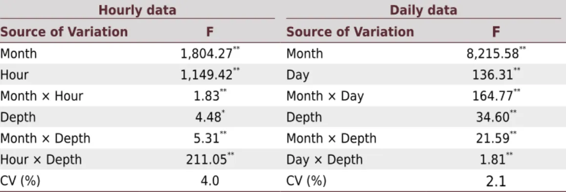
Analysis of variance performed for hourly and daily soil temperature data showed significance through the F-test for the single effects of month, hour or day, depth, and their interactions (Table 2). As soil temperature usually varies at depth, the significant interactions certainly indicate that the responses to monthly, hourly, or daily factors were different for each depth; thus, we decided to analyze and discuss them separately within each depth. The coefficients of variation were low (4.0 and 2.1 %), indicating small variation among data, and variation was lower between days than between hours.
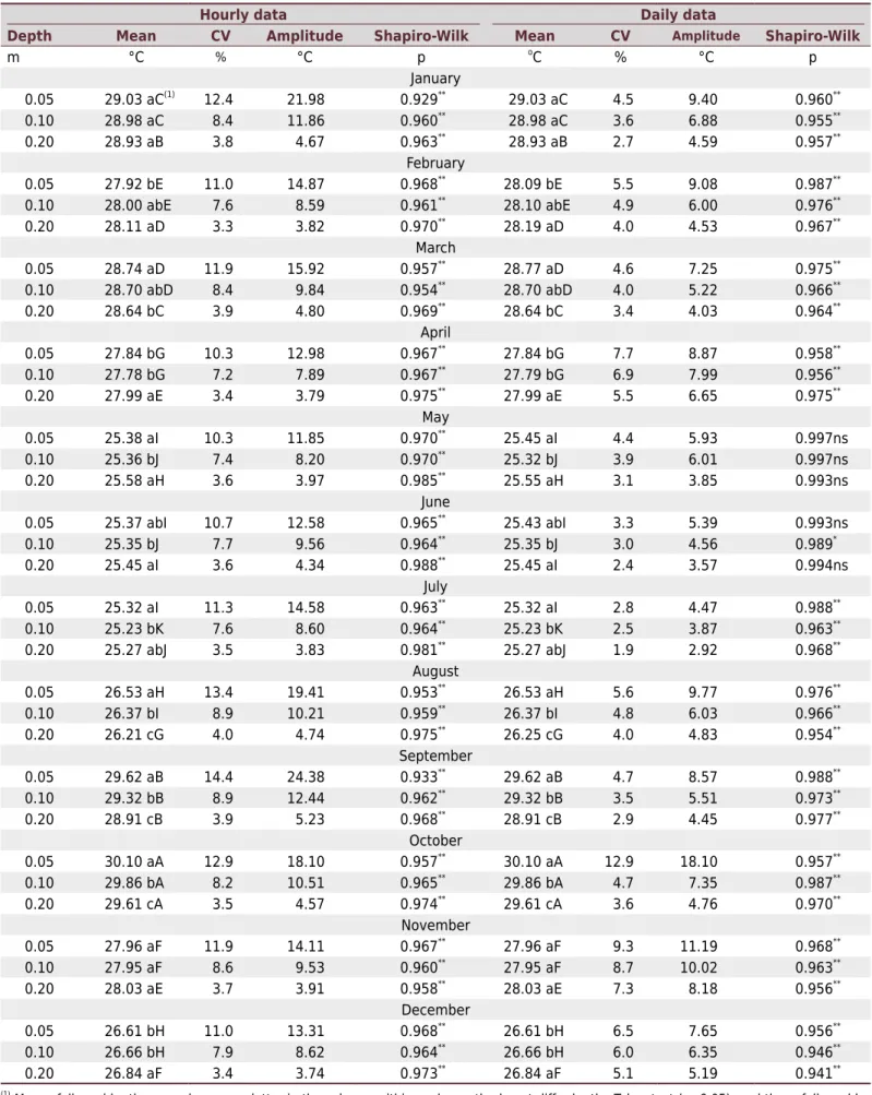
Descriptive statistical analysis for hourly and daily data did not show normal distribution in most of the months for all depths studied, according to the Shapiro-Wilk test (Table 3), except for May at all depths and June at the 0.05 and 0.20 m depths for daily data, which showed normal distribution.
October, September, January, and March showed the highest mean soil temperature readings reaching 46.2, 37.3, and 32.3 °C at the 0.05, 0.10, and 0.20 m depths, respectively, for the hourly data, and 41.5, 34.0, and 32.5 °C for the daily readings (Table 3). The depth of 0.05 m showed the highest thermal amplitude, reaching a maximum of 24.4 °C in September for hourly data, and 18.1 °C in October for daily data. The proximity to the soil surface of this depth eased heat gain and loss (Gasparim et al., 2005).
June and July showed the lowest soil temperature values and amplitude for the hourly and daily data for the depths studied (Table 3), which can be explained by the low air temperature for those months (Figure 1).
Soil temperature variability in relation to mean values can be evaluated by the coefficient of variation (CV) (Diniz et al., 2013a). The variability of the hourly and daily soil temperature per month was inversely related to depth (Table 3). As measurements approached the soil surface, the magnitude of the coefficient of variation increased, as a result of the high thermal amplitude throughout the day and/or the months; therefore, maximum values were recorded at the 0.05 m depth. Even so, CV values for hourly data reached only the mean of the variability range (Pimentel-Gomes and Garcia, 2002), with a minimum of 10.3 % in April and a maximum of 14.4 % in September. For the daily data, soil temperature showed low variability, even in the surface layer, with a minimum CV of 2.8 % in July and a maximum of 9.3 % in November.
Thermal amplitudes in the soil of the months studied, for both the hourly and daily mean data (Table 3), showed lower soil temperature variation with an increase in depth, regardless of the external variables that affect the increase or decrease in heat emission from the soil.
Table 2. F-test of analysis of variance for hourly and daily soil temperature data at three depths
of a Cambissolo Háplico Ta Eutrófico (Cambisol; Inceptisol) from February 04, 2014, to September 30, 2015, in São Gabriel, Irecê Identity Territory, Bahia, Brazil
Hourly data Daily data
Source of Variation F Source of Variation F
Month 1,804.27**
Month 8,215.58**
Hour 1,149.42**
Day 136.31**
Month × Hour 1.83**
Month × Day 164.77**
Depth 4.48*
Depth 34.60**
Month × Depth 5.31** Month × Depth 21.59** Hour × Depth 211.05**
Day × Depth 1.81**
CV (%) 4.0 CV (%) 2.1
*
Table 3. Statistical summary of monthly, hourly, and daily soil temperature at different depths of a Cambissolo Háplico Ta Eutrófico
(Cambisol; Inceptisol), from February 04, 2014 to September 30, 2015, in São Gabriel, Irecê Identity Territory, Bahia, Brazil
Hourly data Daily data
Depth Mean CV Amplitude Shapiro-Wilk Mean CV Amplitude Shapiro-Wilk
m °C % °C p o
C % °C p
January
0.05 29.03 aC(1) 12.4 21.98 0.929** 29.03 aC 4.5 9.40 0.960** 0.10 28.98 aC 8.4 11.86 0.960**
28.98 aC 3.6 6.88 0.955**
0.20 28.93 aB 3.8 4.67 0.963**
28.93 aB 2.7 4.59 0.957**
February 0.05 27.92 bE 11.0 14.87 0.968**
28.09 bE 5.5 9.08 0.987**
0.10 28.00 abE 7.6 8.59 0.961** 28.10 abE 4.9 6.00 0.976** 0.20 28.11 aD 3.3 3.82 0.970**
28.19 aD 4.0 4.53 0.967**
March 0.05 28.74 aD 11.9 15.92 0.957**
28.77 aD 4.6 7.25 0.975**
0.10 28.70 abD 8.4 9.84 0.954**
28.70 abD 4.0 5.22 0.966**
0.20 28.64 bC 3.9 4.80 0.969**
28.64 bC 3.4 4.03 0.964**
April
0.05 27.84 bG 10.3 12.98 0.967** 27.84 bG 7.7 8.87 0.958** 0.10 27.78 bG 7.2 7.89 0.967**
27.79 bG 6.9 7.99 0.956**
0.20 27.99 aE 3.4 3.79 0.975**
27.99 aE 5.5 6.65 0.975**
May 0.05 25.38 aI 10.3 11.85 0.970**
25.45 aI 4.4 5.93 0.997ns 0.10 25.36 bJ 7.4 8.20 0.970** 25.32 bJ 3.9 6.01 0.997ns 0.20 25.58 aH 3.6 3.97 0.985**
25.55 aH 3.1 3.85 0.993ns June
0.05 25.37 abI 10.7 12.58 0.965**
25.43 abI 3.3 5.39 0.993ns 0.10 25.35 bJ 7.7 9.56 0.964**
25.35 bJ 3.0 4.56 0.989*
0.20 25.45 aI 3.6 4.34 0.988**
25.45 aI 2.4 3.57 0.994ns July
0.05 25.32 aI 11.3 14.58 0.963** 25.32 aI 2.8 4.47 0.988** 0.10 25.23 bK 7.6 8.60 0.964**
25.23 bK 2.5 3.87 0.963**
0.20 25.27 abJ 3.5 3.83 0.981**
25.27 abJ 1.9 2.92 0.968**
August 0.05 26.53 aH 13.4 19.41 0.953**
26.53 aH 5.6 9.77 0.976**
0.10 26.37 bI 8.9 10.21 0.959** 26.37 bI 4.8 6.03 0.966** 0.20 26.21 cG 4.0 4.74 0.975**
26.25 cG 4.0 4.83 0.954**
September 0.05 29.62 aB 14.4 24.38 0.933**
29.62 aB 4.7 8.57 0.988**
0.10 29.32 bB 8.9 12.44 0.962**
29.32 bB 3.5 5.51 0.973**
0.20 28.91 cB 3.9 5.23 0.968**
28.91 cB 2.9 4.45 0.977**
October
0.05 30.10 aA 12.9 18.10 0.957** 30.10 aA 12.9 18.10 0.957** 0.10 29.86 bA 8.2 10.51 0.965**
29.86 bA 4.7 7.35 0.987**
0.20 29.61 cA 3.5 4.57 0.974**
29.61 cA 3.6 4.76 0.970**
November 0.05 27.96 aF 11.9 14.11 0.967**
27.96 aF 9.3 11.19 0.968**
0.10 27.95 aF 8.6 9.53 0.960**
27.95 aF 8.7 10.02 0.963**
0.20 28.03 aE 3.7 3.91 0.958**
28.03 aE 7.3 8.18 0.956**
December 0.05 26.61 bH 11.0 13.31 0.968**
26.61 bH 6.5 7.65 0.956**
0.10 26.66 bH 7.9 8.62 0.964**
26.66 bH 6.0 6.35 0.946**
0.20 26.84 aF 3.4 3.74 0.973**
26.84 aF 5.1 5.19 0.941** (1) Means followed by the same lowercase letter in the column, within each month, do not differ by the Tukey test (p<0.05), and those followed by
the same capital letter in the column, for the same depth, do not differ by the Scott-Knott test (p <0.05). *
and ** = significant at 5 % and at 1 %, i.e.,
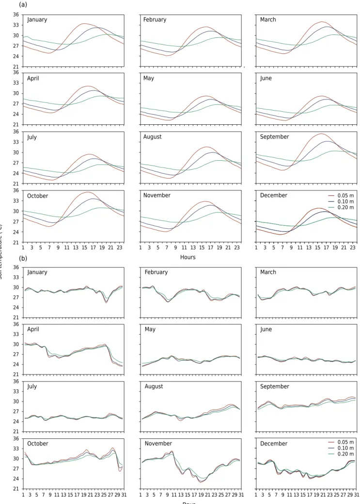
Monthly mean of hourly and daily soil temperature showed higher fluctuation in the layers closer to the surface (Figure 2). In all months, the 0.05 m depth layer showed higher temperature fluctuations throughout the day; the minimum temperature ranged from 22.0 °C in July to 25.6 °C in October between 7 and 8 a.m., and the maximum temperature ranged from 29.3 °C in May and June to 35.5 °C in October, always around 4 p.m. (Figure 2a).
Considering the mean for all months, the lowest hourly values occurred at 7 a.m. and the highest hourly values at 4 p.m. for the 0.05 m depth; at 8 a.m. and 5 p.m. for the 0.10 m depth; and at 10 a.m. and 7 p.m. for the 0.20 m depth (Table 4).
Minimum values between 2 a.m. and 8 a.m. and maximum values between 12 noon and 5 p.m. in a semiarid region in a Neossolo Regolítico at Campina Grande, state of Paraiba, Brazil were found by Diniz et al. (2013a). In the same soil and location, Oliveira et al. (2010) found regions closer to the soil surface showed lowest temperatures around 5 a.m. and maximum temperatures around 2 p.m. In a Latossolo Vermelho-Amarelo in the state of Espírito Santo, Brazil, Belan et al. (2013) also found maximum values in the surface layer between 12 noon and 2 p.m., and Kunz et al. (2002) found that the maximum soil temperature occurred around 4 p.m., which corroborates the results of this study.
There was a one hour lag between the maximum soil temperature in the 0.05 m layer, which occurred at 4 p.m., and that of the 0.10 m layer, which occurred at 5 p.m., as well as a three hour lag in maximum soil temperature between the same 0.05 m layer and the 0.20 m layer, which occurred at 7 p.m., for most of the months (Figure 2a). This is directly related to the low heat conductivity of the soil when dry, which is the prevailing condition in the region. Therefore, the 0.10 m layer for all months showed a soil temperature fluctuation closer to the 0.05 m layer than to the 0.20 m layer. Similar results were found by Belan et al. (2013) and Diniz et al. (2014), who found that maximum temperatures occurred at different times. The delay from surface to deeper depths showed that the heat wave requires a certain time period to propagate in the soil because of slow heat conduction capacity through the vertical soil profile, as mentioned above.
The daily data from February, April, November, and December (Figure 2b) showed a significant decrease in soil temperature due to rainfall, which was in greater amount in these months than in the other months (Figure 1). According to Brady and Weil (2013), the lower temperatures of a water-saturated soil are due, in part, to water evaporation - a process that consumes a lot of heat - and, in part, to high specific heat in water-saturated soil, which is 1 cal g-1, whereas specific heat in dry soil is 0.2 cal g-1. Furthermore, according
to these authors, soil temperature in the few centimeters above saturated soil is usually 3 to 6 °C lower than that of dry soil or slightly moist soil. The present study also showed these results because the lowest mean daily soil temperature at the 0.05 m depth was 25.7 °C for February, 23.4 °C for April, 23.1 °C for November, and 24.1 °C for December, which represents a drop of 3.3 to 5 °C for months with low rainfall compared to months with more abundant rain. In studies performed by Diniz et al. (2013a), the months of lower soil temperatures were precisely the months with higher rainfall.
From May to July, the daily soil temperature was lower and more constant (Figure 2b), with generally no sudden temperature gains or loss for the three depths studied. This can be attributed to the effects of low rainfall and atmospheric temperature, which exhibited lower monthly means in these months (Figure 1).
Figure 2. The hourly (a) and daily (b) monthly mean of soil temperature at three different depths of a Cambissolo Háplico Ta Eutrófico
(Cambisol; Inceptisol), from February 04, 2014, to September 30, 2015, in São Gabriel, Irecê Identity Territory, Bahia, Brazil.
Soil temperatur
e
(
o C)
Hours
Days
March February
January
21 24 27 30 33 36
June
September May
April
21 24 27 30 33 36
August July
21 24 27 30 33 36
December November
October
21 24 27 30 33 36
1 3 5 7 9 11 13 15 17 19 21 23 25 27 29 31 1 3 5 7 9 11 13 15 17 19 21 23 25 27 29 31 1 3 5 7 9 11 13 15 17 19 21 23 25 27 29 31
March
June February
January
21 24 27 30 33 36
21 24 27 30 33 36
21 24 27 30 33 36
21 24 27 30 33 36
September May
April
August July
(a)
November October
1 3 5 7 9 11 13 15 17 19 21 23 1 3 5 7 9 11 13 15 17 19 21 23 1 3 5 7 9 11 13 15 17 19 21 23
December
0.05 m 0.10 m 0.20 m 0.05 m 0.10 m 0.20 m
Soil temperature fluctuations, however subtle they may be, can significantly affect plant growth and development. Specifically in regard to castor bean, the main crop of the Irecê Identity Territory, the optimum soil temperature for seed germination is about 29 °C. According to Lucena et al. (2014), at 29 °C castor bean seedlings required an mean of 8.6 days to achieve 50 % emergence, whereas at 23 °C this took 12.8 days, and at 38 °C, 24.4 days. The present study showed that, for most days, soil temperature was within the range recommended for good castor bean emergence.
The studied soil had a dark color (yellowish red when dry and dark reddish brown when wet), which contributes to an increase in soil surface temperature during the day through high absorption of solar energy and lower reflectance (Dalmolin et al., 2005). Soil bulk density is an additional property that affects soil heat transfer. In table 1 it can be seen that soil bulk density increased with depth, ensuring lower soil thermal amplitude in the deeper layers, since the thermal conductivity of mineral particles is higher than that of air particles (Brady and Weil, 2013). As shown in table 1, the quantity of micropores, i.e., the pores that retain water, was higher than that of macropores. In the rainy season, this condition contributes to lower soil thermal amplitude in the surface and subsurface.
The regression equations between air temperature and soil temperature data (Table 5)
showed the coefficient of determination (R2) significant at 1 % for all months for the
0.05 m depth, and lower R2 values significant at 5 % or not significant for the 0.10 and 0.20 m depths. This confirmed that soil temperature at the 0.05 m depth is more affected by air temperature, less affected at the 0.10 m depth, and not affected at the 0.20 m
Table 4. Mean hourly soil temperature for all months and for different depths, from February 04,
2014, to September 30, 2015, in a Cambissolo Háplico Ta Eutrófico (Cambisol; Inceptisol) in São Gabriel, Irecê Identity Territory, Bahia, Brazil
Depth
0.05 m 0.10 m 0.20 m
Hour Soil temperature(1)
Hour Soil temperature(1)
Hour Soil temperature(1)
°C °C °C
4 p.m. 32.2 a 17 30.8 a 19 28.8 a
3 p.m. 32.0 a 18 30.7 b 18 28.8 b
5 p.m. 31.8 a 16 30.6 b 20 28.8 b
2 p.m. 31.4 b 19 30.1 c 21 28.6 c
6 p.m. 31.1 c 15 30.0 c 17 28.5 d
1 p.m. 30.4 d 20 29.4 d 22 28.5 d
7 p.m. 30.0 e 14 29.2 e 23 28.3 e
12 a.m. 29.0 f 21 28.8 f 0 28.1 f
8 p.m. 29.0 f 22 28.2 g 16 28.0 f
9 p.m. 28.1 g 13 28.2 g 1 27.8 g
11 a.m. 27.5 h 23 27.7 h 2 27.6 h
10 p.m. 27.4 h 0 27.2 i 3 27.4 i
11 p.m. 26.8 i 12 27.1 i 15 27.4 i
12 p.m. 26.3 j 1 26.8 j 4 27.2 j
10 a.m. 26.0 k 2 26.4 k 5 27.0 k
1 a.m. 25.8 k 11 26.1 l 14 26.9 l
2 a.m. 25.4 l 3 26.0 l 6 26.8 m
3 a.m. 25.0 m 4 25.7 m 7 26.6 n
9 a.m. 24.7 n 5 25.4 n 13 26.6 n
4 a.m. 24.6 n 10 25.3 n 8 26.4 o
5 a.m. 24.3 o 6 25.1 o 12 26.3 o
8 a.m. 23.9 p 9 24.8 p 9 26.3 p
6 a.m. 23.9 p 7 24.8 p 11 26.2 p
7 a.m. 23.7 p 8 24.7 q 10 26.2 p
(1) Means followed by the same letter in the column, for the same depth, do not differ by the Scott-Knott test
depth. This occurs because of low soil heat diffusivity, especially in soil with low water quantity, which is the condition in the region studied most of the time. In this case, there is a delay in propagation of the heat wave in the soil, which contributes to decreasing the relationship between air temperature and soil temperature at greater depth. Similar results were found by Belan et al. (2013) under conditions of soil without cover, with high correlation between air temperature and soil temperature at the 0.02 and 0.05 m depths, and poor correlation at the 0.20 m depth. Azevedo and Galvani (2003) and Carvalho et al. (2009) found similar results at depths closest to the surface; however, these authors found a higher R² value at the 0.20 m depth.
Evaluation of the predictive capacity of the linear regression equations developed between air temperature and soil temperature for the depth of 0.05 m for July, September, and December 2016 (Table 5) showed a higher occurrence of data overestimation than underestimation (Figure 3). The values calculated for RMSE considerably different from 0 (1.748) and the concordance coefficient of Willmott (1981) below 1 (0.858) numerically expressed the over- and underestimation of values by the use of the regression equation (Figure 3). Even so, the c coefficient of Camargo and Sentelhas (1997) was 0.740, indicating good performance of the equations that were developed.
Awe at al. (2015) observed linear correlations between mean daily air and soil temperature (0.025 m) with R2 ranging from 0.80 to 0.88. In the present study, R2 was 0.743 (Figure 3),
but using all hourly values of air and soil temperature (0.05 m), so it can be considered comparatively as satisfactory.
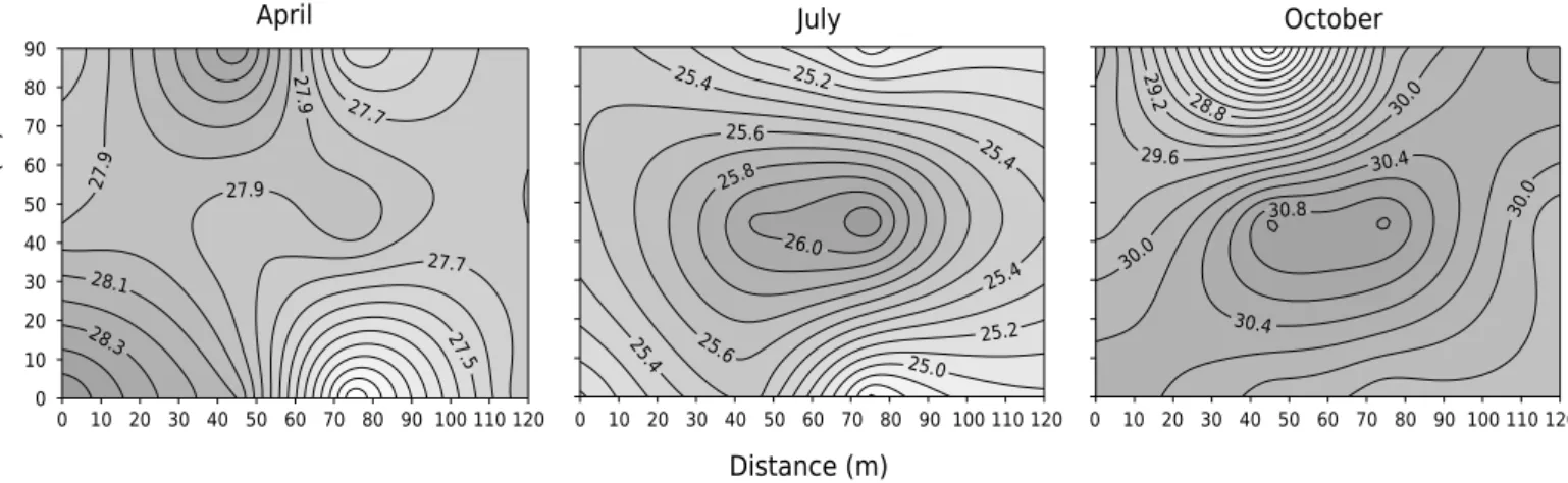
The spatial distribution of soil temperature at the 0.05 m depth for April, July, and October (Figure 4) displays intermediate, minimum, and maximum daily temperature amplitudes, respectively. Although there are differences among thematic maps for each of these months, the spatial thermal amplitude within each month can be considered low, with the minimum and maximum values reaching 26.8 and 28.5 °C in April, 24.8 and 26.1 °C in July, and 27.7 and 30.9 °C in October. The same behavior was observed in the remaining
Table 5. Linear regression equations developed for air and soil temperature from April, 2015 to March, 2016, considering three
depths of Cambissolo Háplico Ta Eutrófico (Cambisol; Inceptisol), in São Gabriel, Irecê Identity Territory, Bahia, Brazil
Month
Depth
0.05 m 0.10 m 0.20 m
Equation R² Equation R² Equation R²
January ŷ = 0.829 x + 6.471 0.718** ŷ = 0.554 x + 10.988
0.506* ŷ = 0.326 x + 16.820
0.245 ns
February ŷ = 0.590 x + 13.140 0.757** ŷ = 0.276 x + 18.730
0.354 ns ŷ = 0.049 x + 24.470 0.027 ns
March ŷ = 0.450 x + 18.980 0.641**
ŷ = 0.237 x + 21.990 0.362*
ŷ = 0.009 x + 27.862 0.002 ns
April ŷ = 0.719 x + 10.120 0.738**
ŷ = 0.457 x+ 16.810 0.466*
ŷ = 0.121 x+ 25.480 0.081 ns
May ŷ = 0.639 x + 11.540 0.725**
ŷ = 0.3500 x + 16.630 0.390 ns ŷ = 0.058 x + 23.770 0.021 ns
June ŷ = 0.530 x + 13.820 0.697**
ŷ = 0.246 x + 18.000 0.334 ns ŷ = 0.021 x + 23.160 0.007 ns
July ŷ = 0.531 x + 13.720 0.699**
ŷ = 0.230 x + 18.150 0.311 ns ŷ = 0.003 x + 23.170 0.000 ns
August ŷ = 0.615 x + 12.780 0.754** ŷ = 0.302 x + 17.380 0.395* ŷ = 0.067 x + 22.535 0.047 ns
September ŷ = 0.615 x + 14.570 0.819** ŷ = 0.270 x + 20.420 0.419* ŷ = 0.020 x + 26.380 0.008 ns
October ŷ = 0.675 x + 14.110 0.831** ŷ = 0.295 x + 21.060
0.451* ŷ = 0.027 x + 27.770
0.014 ns
November ŷ = 0.736 x + 12.030 0.760** ŷ = 0.349 x + 19.840
0.423* ŷ = 0.055 x + 27.770
0.032 ns
December ŷ = 0.660 x + 13.785 0.803**
ŷ = 0.332 x + 20.070 0.495*
ŷ = 0.038 x + 28.120 0.026 ns
Every month ŷ = 0.735 x + 10.422 0.736**
ŷ = 0.452 x + 15.150 0.469*
ŷ = 0.227 x + 20.703 0.182 ns
R² = coefficient of determination; ŷ = soil temperature; x = air temperature; ns = not significant; *
months of the year for the 0.05 m depth, the spatial thermal amplitude was lower for the 0.10 and 0.20 m depths, and the similarity between monthly maps increased with depth. Therefore, we chose to present only the graphics included in figure 4.
The CV has been the measure most used to quantify the variability of soil properties (Oliveira Junior, 2011), even allowing the minimum number of measurement points in an area to be calculated in order to estimate a soil property value at a determined level of accuracy. Thus, the higher the CV, the greater the number of measurement points to be considered (Amaro Filho et al., 2007).
As for hourly soil temperature data, with the aim of high reliability (α = 0.05), low numbers of measurement points in an area were determined for evaluating soil temperature (Figure 5a) at 10 % variation from the mean.
As the mean estimated error increases, the number of measurement points decreases, and, thus, it is possible to estimate the soil temperature in the area with three measurement points for 0.05 m, and one point for the 0.10 and 0.20 m depths, for variations from the mean of 15 % or more (Figure 5a). A variation of up to 20 % does not imply high error in the true population mean (Amaro Filho et al., 2007; Guarçoni et al., 2007; Oliveira et al., 2007).
20 24 28 32 36 40
20 24 28 32 36 40
1:1
ŷ = 0.8933x** + 3.0405
R2
= 0.743
Estimated soil temperatu
re
(
o C)
Observed soil temperature (o
C)
Figure 3. Evaluation of the predictive capacity of the linear regression equations developed
between air temperature and soil temperatures to the depth of 0.05 m of a Cambissolo Háplico
Ta Eutrófico (Cambisol; Inceptisol) for July, September, and December 2016, in São Gabriel, Irecê Identity Territory, Bahia, Brazil.
Distance (m
)
0 10 20 30 40 50 60 70 80 90 100 110 120
0 10 20 30 40 50 60 70 80 90
27.9 27.9
28.1
28.3
27.7 27.7 27.9
27 .5
April
Distance (m)
0 10 20 30 40 50 60 70 80 90 100 110 120
25.4 25.2
25.6
25.8
26.0
25.4
25.4
25.2
25.0 25.6
25.4
July
0 10 20 30 40 50 60 70 80 90 100 110 120
28.8 29.2
29.6
30.0
30.0
30.0
30.4
30.4
30.8 October
Figure 4. Spatial distribution of soil monthly mean temperature at a 0.05 m depth of a Cambissolo Háplico Ta Eutrófico (Cambisol;
The lowest CV for daily soil temperature data (Table 3) significantly affected the number of measurement points required to evaluate soil temperature in an area (Figure 5b). For 0.05, 0.10, and 0.20 m depths, 6, 4, and 3 points were estimated, respectively, for variation of 5 % from the mean, and 1 point for 15 % variation or more for all the depths measured. Souza (1992) found similar results to estimate clay, soil bulk density, and soil moisture, requiring one measurement point for 15, 20, 25, and 30 % variations. Amaro Filho et al. (2007) estimated one measurement point for 15 % or more variation from the mean for soil bulk density.
In research studies, the use of the estimated number of points for 10 % variation from the mean is suggested, aiming to reduce the effort of measurement without significantly affecting the accuracy. In production areas, considering reliable data and lower cost, use of the estimated number of points for 15 % variation is suggested.
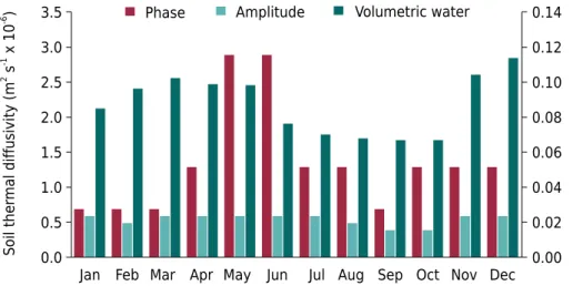
September exhibited the lowest soil temperature diffusivity by the amplitude method, with a value of 4.80 × 10⁻⁷ m2 s-1 (Figure 6). This probably occurred due to the lack of
rainfall in that month. Compared to the other months, September showed less heat
transfer capacity. January showed the highest thermal diffusivity, with 6.93 × 10⁻⁷ m2 s-1.
Jan Feb Mar Apr May Jun Jul Aug Sep Oct Nov Dec 0.0
0.5 1.0 1.5 2.0 2.5 3.0 3.5
0.00 0.02 0.04 0.06 0.08 0.10 0.12 0.14 Phase Amplitude Volumetric water
Soil ther
mal diffusivity (m
2 s -1 x 10 -6 )
Vo
lumetric water (m
3
m
-3
)
Figure 6. Monthly means of soil thermal diffusivity at the 0.05 and 0.20 m depths of a Cambissolo
Háplico Ta Eutrófico (Cambisol; Inceptisol) estimated based on soil temperature data recorded from February 04, 2014, to September 30, 2015, in São Gabriel, Irecê Identity Territory, Bahia, Brazil. 0
5 10 15 20 25 30
5 10 15 20 25 30 5 10 15 20 25 30
0.05 m 0.10 m 0.20 m
Number of measur
ement points
Difference from the mean (%)
(a) (b)
Figure 5. Minimum number of measurement points required to estimate the monthly hourly (5a) and daily (5b) soil temperature
to several difference from the mean in percentage, considering daily data of soil temperature of a Cambissolo Háplico Ta Eutrófico
In studies performed by Diniz et al. (2013b), also in semi-arid conditions and under the same method at depths from 0.10 to 0.20 m, the lowest and highest diffusivity values occurred in December (0.52 × 10⁻⁶ m2 s-1) and August (0.78 × 10⁻⁶ m2 s-1),
respectively. In another study developed by Diniz et al. (2014) in the state of Paraiba, Brazil, considering depths from 0.05 to 0.15 m, October showed the lowest thermal
diffusivity (0.59 × 10⁻⁶ m2 s-1) and June showed the highest (1.11 × 10⁻⁶ m2 s-1) in 2010.
According to the authors, June had the greatest rainfall; therefore, the soil pore space was filled with water, providing greater heat conduction capacity. December had the
lowest diffusivity in 2011 (0.74 × 10⁻⁶ m² s-1) and January had the highest (1.14 ×
10-6 m² s-1), similar to this study. The mean results found by the amplitude method for
monthly means (6.08 × 10⁻⁷ m² s-1) and for the eight periods studied (8.68 × 10⁻⁷ m2 s-1)
were similar to those obtained by Soares et al. (2014) and Oliveira et al. (2015), which were 2.43 × 10⁻⁷ and 5.25 × 10⁻⁷ m2 s-1, respectively, converging to a diffusivity value
in the order of magnitude of 10-7. In general, soils have thermal diffusivity from 10-7
to 10-8 m2 s-1, confirming the effectiveness of the amplitude method in relation to the
phase method (Amaro Filho et al., 2008).
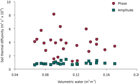
In the phase method, there was higher thermal diffusivity when the soil moisture was lower, as well as the contrary, although there was no well-defined ratio between both variables. In the amplitude method, the diffusivity showed lower values, which remained more constant and without large fluctuations with an increase in soil moisture (Figure 7). Therefore, it is assumed that other soil properties such as clay-loam soil texture, the predominance of micropores (Table 1), and a considerable presence of iron oxides, indicated by yellowish red (5YR 4/6, dry) and dark reddish brown (5YR 3/4, wet) colors, allowed greater proximity among the soil particles. This provided for higher thermal diffusivity even under low soil moisture conditions. A similar result was found by Rezende (2010), who evaluated three vegetation types in Serra Sul in Pará, Brazil, and observed a higher thermal diffusivity value for the amplitude and phase methods in the area with a lower soil moisture value throughout the year. The authors observed that the soil in this region has predominance of iron oxides in its composition, which allows greater proximity of particles and, consequently, higher thermal diffusivity.
Soil ther
mal diffusivity (m
2 s
-1 x 10
-6 )
Volumetric water (m3 m-3) 0
2 4 6 8 10
0.04 0.08 0.12 0.16 0.20
Phase
Amplitude
Figure 7. Soil thermal diffusivity at the 0.05 and 0.20 m depths depending on the soil moisture
CONCLUSIONS
On most days, the soil temperature was at the level recommended for castor bean.
October and July, respectively, showed maximum and minimum hourly and daily soil temperatures, and the maximum soil temperature values occurred at 4 p.m. (0.05 m), 5 p.m. (0.10 m), and 7 p.m. (0.20 m).
Soil temperature variability is low, requiring few measurement points to estimate this factor in an area.
The amplitude method led to soil thermal diffusivity values compatible with results in the literature. The absence of a relationship between thermal diffusivity and soil moisture is attributed to the clay-loam soil texture, predominance of micropores, and iron oxides allowing greater approximation to the soil particles, with high thermal diffusivity even under low soil moisture conditions.
REFERENCES
Amaro Filho J, Assis Júnior RN, Mota JCA. Física do solo: conceitos e aplicações. Fortaleza: Imprensa Universitária, 2008.
Amaro Filho J, Negreiros RFD, Assis Júnior RN, Mota JCA. Amostragem e variabilidade espacial
de atributos físicos de um Latossolo Vermelho em Mossoró, RN. Rev Bras Cienc Solo.
2007;31:415-22. https://doi.org/10.1590/S0100-06832007000300001
Awe GO, Reichert JM, Wendroth OO. Temporal variability and covariance structures of soil
temperature in a sugarcane field under different management practices in southern Brazil.
Soil Till Res. 2015;150:93-106. https://doi.org/10.1016/j.still.2015.01.013
Azevedo TR, Galvani E. Ajuste do ciclo médio mensal horário da temperatura do solo em função da temperatura do ar. Rev Bras Agrometeorologia. 2003;11:123-30.
Belan LL, Xavier TMT, Torres H, Toledo JV, Pezzopane JEM. Dinâmica entre temperaturas do ar
e do solo sob duas condições de cobertura. Rev Acad: Cienc Agrar Ambient. 2013;11:S147-54. https://doi.org/10.7213/academica.10.S01.AO17
Beltrão NEM, Brandão ZN, Amaral JAB, Araújo AE. Clima e solo. In: Azevedo DMP, Beltrão NEM, editores. O agronegócio da mamona no Brasil. 2.ed rev ampl. Campina Grande: Embrapa Algodão - Brasília, DF: Embrapa Informação Tecnológica; 2007. p.73-93.
Brady NC, Weil RR. Elementos da natureza e propriedades dos solos. 3. ed. Porto Alegre: Bookman, 2013.
Brasil. Ministério da Agricultura, Pecuária e Abastecimento, Companhia Nacional de Abastecimento. Conjuntura mensal da mamona, safra 2015/2016 [internet]. Brasília, DF: Ministério da Agricultura, Pecuária e Abastecimento; 2017 [acesso em 20 fev 2017]. Disponível em: http://www.conab.gov.br.
Brasil. Ministério do Desenvolvimento Agrário. Programa nacional de produção e uso de biodiesel: inclusão social e desenvolvimento territorial [internet]. Brasília, DF: Ministério do Desenvolvimento Agrário; 2011 [acesso em 07 mar 2017]. Disponível em: http://www.mda.gov.
br/sitemda/sites/sitemda/files/user_arquivos_64/Biodiesel_Book_final_Low_Completo.pdf.
Camargo AP, Sentelhas PC. Avaliação do desempenho de diferentes métodos de estimativa da evapotranspiração potencial no estado de São Paulo, Brasil. Rev Bras Agrometeorologia. 1997;5:89-97.
Carneiro RG, Moura MAL, Silva VPR, Silva Junior RS, Andrade AMD, Santos AB. Variabilidade da temperatura do solo em função da liteira em fragmento remanescente de mata atlântica.
Rev Bras Eng Agr Amb. 2014;18:99-108. https://doi.org/10.1590/S1415-43662014000100013
Cartaxo WV, Beltrão NEM, Silva ORRF, Severino LS, Auassuna ND, Soares JJ. O cultivo da
Carvalho HP, Honório DF, Rabelo PG. Estimativa da temperatura de um solo coberto com grama em função da temperatura do ar. In: Anais da 9a Jornada de ensino, pesquisa e extensão JEPEX 9 [CD-ROM]; 2009; Recife. Recife: Universidade Federal Rural de Pernambuco; 2009.
Cline MG. Principles of soil sampling. Soil Sci. 1944;58:275-88.
Dalmolin RSD, Gonçalves CN, Klamt E, Dick DP. Relação entre os constituintes do solo e seu comportamento espectral. Cienc Rural. 2005;35:481-9.
https://doi.org/10.1590/S0103-84782005000200042
Danelichen VHM, Biudes MS. Avaliação da difusividade térmica de um solo no norte do
Pantanal. Cien Natura. 2011;33:227-40.
Diniz JMT, Aranha TRBT, Sousa EP, Wanderley JAC, Sousa EP, Maracajá PB. Avaliação da difusividade térmica do solo de Campina Grande-PB - Brasil. Agropec Cient Semiarido. 2013b;9:55-60.
Diniz JMT, Carneiro RG, Alvino FCG, Sousa EP, Sousa EP, Sousa Júnior JR. Avaliação do comportamento térmico diário do solo de Campina Grande-PB. Agropec Cient Semiarido. 2013a;9:77-82.
Diniz JMT, Dantas RT, Fideles Filho J. Variabilidade espaço-temporal da temperatura
e difusividade térmica do solo de Lagoa Seca-PB. Rev Ambient Agua. 2014;9:722-36. https://doi.org/10.4136/ambi-agua.1474
Dourado-Neto D, Timm LC, Oliveira JCM, Klaus R, Bacchi OOS, Tominaga TT, Cássaro FAM. State-space approach for the analysis of soil water content and temperature in a sugarcane crop. Sci Agric. 1999;56:1215-21. http://dx.doi.org/10.1590/S0103-90161999000500025
Ferreira DF, Cargnelutti Filho A, Lúcio AD. Procedimentos estatísticos em planejamentos
experimentais com restrição à casualização. Viçosa: Sociedade Brasileira de Ciência do Solo;
2012. Boletim Informativo, 03.
Gasparim E, Ricieri RP, Silva SL, Dallacort R, Gnoatto E. Temperatura no perfil do solo
utilizando duas densidades de cobertura e solo nu. Acta Sci-Agron. 2005;27:107-14. https://doi.org/10.4025/actasciagron.v27i1.2127
Gee GW, Or D. Particle-size analysis. In: Dane JH, Topp GC, editors. Methods of soil analysis. Physical methods. Madison: Soil Science Society of America; 2002. Pt. 4. p.255-93.
Grossman RB, Reinsch TG. Bulk density and linear extensibility. In: Dane JH, Topp GC, editors. Methods of soil analysis. Physical methods. Madison: Soil Science Society of America; 2002. Pt. 4. p.201-28.
Guarçoni MA, Alvarez V VH, Novais RF, Cantarutti RB, Leite HG, Freire FM. Diâmetro
de trado necessário à coleta de amostras num Cambissolo sob plantio direto ou sob plantio convencional antes ou depois da aração. Rev Bras Cienc Solo. 2007;31:947-59. https://doi.org/10.1590/S0100-06832007000500012
Instituto Nacional de Meteorologia - Inmet. Dados meteorológicos, 2015 [acesso em 20 fev 2017]. Disponível em: http://www.inmet.gov.br/portal/.
Kunz M, Santi G, Reinert D, Reichert JM, Sequinato L, Osório Filho B. Temperatura do solo
influenciado pelo sistema de manejo dado ao solo para a cultura do feijoeiro. In: Anais da XIV Reunião Brasileira de Manejo e Conservação do Solo e da Água [CD-ROM]; 2002; Cuiabá.
Cuiabá: Sociedade Brasileira de Ciência do Solo; 2002. p.6.
Lucena AMA, Severino LS, Correia FG, Farias AL, Arriel NHC. Influência da temperatura do substrato sobre a emergência de plântulas de mamona e gergelim. In: Anais do VI Congresso
Brasileiro de Mamona - III Simpósio Internacional de Oleaginosas Energéticas; 2014; Fortaleza. Campina Grande: Embrapa Algodão; 2014. p.237.
Oliveira DB, Neto NAA, Soares WA. Estimativas da difusividade térmica e do fluxo de calor de
um solo no agreste Pernambucano. Rev Bras Geogr Fis. 2015;8:1053-67.
Oliveira FHT, Arruda JA, Silva IF, Alves JC. Amostragem para avaliação da fertilidade do solo em função do instrumento de coleta das amostras e de tipos de preparo do solo. Rev Bras Cienc Solo. 2007;31:973-83. https://doi.org/10.1590/S0100-06832007000500014
Oliveira Junior JC. Variabilidade espacial de atributos físicos, químicos e mineralógicos de solos
Oliveira LB. Determinação da macro e microporosidade pela “mesa de tensão” em amostras de solo com estrutura indeformada. Pesq Agropec Bras. 1968;3:197-200.
Oliveira SS, Fideles Filho J, Oliveira SV, Araújo TS. Difusividade térmica do solo de Campina
Grande para dois períodos do ano. Rev Geogr. 2010;27:179-89.
Paiva AQ, Souza LS, Fernandes Filho EI, Souza LD, Schaefer CEGR, Costa LM, Lopes TJ, Sousa
DV. Mudança do uso da terra e dinâmica de carbono orgânico do solo no Platô de Irecê, Bahia. Geografia. 2015;40:85-99.
Pimentel-Gomes F, Garcia CH. Estatística aplicada a experimentos agronômicos e florestais.
Piracicaba: Fealq; 2002.
Prevedello CL. Energia térmica do solo. In: van Lier QJ, editor. Física do solo. Viçosa, MG:
Sociedade Brasileira de Ciência do Solo, 2010. p. 177-211.
Queiroga VP, Santos RF, Queiroga DAN. Levantamento da produção de mamona (Ricinus
communis L.) em uma amostra de produtores em cinco municípios do estado da Bahia. Rev
Agro@mbiente On-line. 2011;5:148-57. https://doi.org/10.18227/1982-8470ragro.v5i2.409
Rao TVR, Silva BB, Moreira AA. Características térmicas do solo em Salvador, BA. R Bras Eng
Agric Ambiental. 2005;9:554-9. https://doi.org/10.1590/S1415-43662005000400018
Reichardt K, Timm LC. Solo, planta e atmosfera: conceitos, processos e aplicações. 2. ed. Barueri: Editora Manole; 2012.
Reichert JM, Reinert DJ, Braida JA. Qualidade dos solos e sustentabilidade de sistemas agrícolas. Cienc Ambient. 2003;27:29-48.
Rezende LAL. Reabilitação de campos ferruginosos degradados pela atividade minerária no
quadrilátero ferrífero [dissertação]. Viçosa, MG: Universidade Federal de Viçosa; 2010.
Ribeiro S, Chaves LHG, Guerra HOC, Gheyi HR, Lacerda RD. Resposta da mamoneira cultivar BRS-188 Paraguaçu à aplicação de nitrogênio, fósforo e potássio. Rev Cienc Agron. 2009;40:465-73.
Silva FBR, Riché GR, Tonneau JP, Souza Neto NC, Brito LTL, Correia RC, Cavalcanti AC, Silva FHBB, Silva AB, Araújo Filho JC, Leite AP. Zoneamento agroecológico do Nordeste: diagnóstico do quadro natural e agrossocioeconômico. Petrolina: Embrapa-CPATSA/Recife: Embrapa/CNPS. 1993. (Documentos, 80).
Silva VR, Reichert JM, Reinert DJ. Variação na temperatura do solo em três
sistemas de manejo na cultura do feijão. Rev Bras Cienc Solo. 2006;30:391-9. http://dx.doi.org/10.1590/S0100-06832006000300001
Soares WA, Antonino ACD, Lima JRS, Lira CABO. Comparação de seis algoritmos para a determinação da difusividade térmica de um Latossolo Amarelo. Rev Bras Geogr Fis. 2014;7:146-54.
Soil Survey Staff. Keys to soil taxonomy. 12th ed. Washington, DC: United States Department of
Agriculture, Natural Resources Conservation Service; 2014.
Souza LS. Variabilidade espacial do solo em sistema de manejo [tese]. Porto Alegre:
Universidade Federal do Rio Grande do Sul; 1992.
Superintendência de Estudos Econômicos e Sociais da Bahia - SEI. Dinâmica sociodemográfica da Bahia: 1980-2002. V II. Salvador: SEI; 2003. (Estudos e pesquisas; 60).
Willmott CJ. On the validation of models. Phys Geogr, 1981;2:184-94.
World Reference Base for Soil Resources - WRB: International soil classification system for