RBRH, Porto Alegre, v. 23, e24, 2018
Scientific/Technical Article
https://doi.org/10.1590/2318-0331.231820170115
Soil variables as auxiliary information in spatial prediction of shallow water table
levels for estimating recovered water volume
Variáveis do solo como informação auxiliar para predição espacial do nível freático superficial aplicada na estimativa do volume de água recuperado
Lucas Vituri Santarosa1 and Rodrigo Lilla Manzione2
1Programa de Pós-graduação em Agronomia, Faculdade de Ciências Agronômicas, Universidade Estadual Paulista, Botucatu, SP, Brasil
²Faculdade de Ciências e Engenharia de Tupã, Universidade Estadual Paulista, Tupã, SP, Brasil
E-mails: lucasviturisantarosa@gmail.com (LVS), rlmanzione@gmail.com (RLM)
Received: August 02, 2017 - Revised: January 18, 2018 - Accepted: May 12, 2018
ABSTRACT
Spatial data became increasingly utilized in many scientific fields due to the accessibility of monitoring data from different sources.
In the case of hydrological mapping, measurements of external environmental conditions, such as soil, climate, vegetation, are often available in addition to the measurements of water characteristics. An integrated modelling approach capable to incorporate multiple input data sets that may have heterogeneous geometries and other error characteristics can be achieved using geostatistical techniques. In this study, different physical hydric properties of soils extensively sampled and topography were used as auxiliary information for making optimal, point-level inferences of water table depths in forest areas. We used data from 48 wells in the Bauru Aquifer System in the Santa Bárbara Ecological Station (EEcSB), in the municipality of Aguas de Santa Bárbara in São Paulo State, Brazil. Using the resistance of soil to penetration and topography as auxiliary variables helped reduce prediction errors. With the generated maps, it was possible to estimate the volumes of water recovered from the water table in two periods during the monitoring period. These values
showed that 30% of the recovered volume would be sufficient for a three-month supply of water for a population of 30,000 inhabitants. Therefore, this raises the possibility of using areas such as the EEcSB as strategic supplies in artificial recharging management.
Keywords: Data fusion; Groundwater management; Geostatistics; Bauru Aquifer System; Groundwater recharge.
RESUMO
Os dados espaciais tornaram-se cada vez mais utilizados em muitos campos científicos devido ao acesso à resultados do monitoramento
de diferentes fontes. No caso do mapeamento hidrológico, medidas de condições ambientais externas, como solo, clima, vegetação, estão frequentemente disponíveis, além das medidas das características da água. Uma abordagem de modelagem integrada capaz de incorporar vários conjuntos de dados de entrada que podem ter geometrias heterogêneas e outras características de erro que pode ser alcançada usando técnicas geoestatísticas. Neste estudo, foram utilizadas diferentes propriedades físicas dos solos amplamente
amostrados e a topografia como informação auxiliar para fazer inferências ótimas das profundidades do nível freático em área florestal.
Utilizou-se dados de 48 poços no Sistema Aquífero Bauru na Estação Ecológica de Santa Bárbara (EEcSB), no município de Águas
de Santa Bárbara, no Estado de São Paulo, Brasil. O uso da resistência do solo à penetração e a topografia como variáveis auxiliares
ajudou a reduzir erros de predição. Com os mapas gerados, foi possível estimar os volumes de água recuperados no lençol freático
em dois períodos durante o monitoramento. Estes valores mostraram que 30% do volume recuperado seria suficiente para suprir a
demanda por água por três meses para uma população de 30 mil habitantes. Portanto, isso levanta a possibilidade de usar áreas como
o EEcSB como suprimentos estratégicos na gestão de recarga artificial.
INTRODUCTION
The future of natural resources has been the subject of
much reflection in relation to the modern way of life, with the
imminent scarcity of water resources among the greatest causes for concern. Shallow groundwater systems are vitally important to humankind as a source of water, for maintaining river discharge, and for sustaining wetland and riparian ecosystems. When shallow
groundwater systems are unconfined, they are vulnerable to
anthropogenic contamination. It is therefore important for hydrogeologists and natural resource managers to understand the processes of the unsaturated zone that link human activity at the soil surface with the underlying groundwater, and vice versa (DILLON; SIMMERS, 1998). Thus, the strategic importance of groundwater resources has increased, stimulating the development
of efficient methods for their measurement and monitoring.
Such techniques must be capable of assessing the quantity of groundwater resources and the seasonality effects and possible alterations in climatic conditions. This understanding would promote a balance of the interests around the multiple functions attributed to groundwater, making the knowledge regarding the very important spatiotemporal dynamics of the groundwater (VON ASMUTH; KNOTTERS, 2004).
Robust data collection is a fundamental requirement for a
monitoring system intended to reflect a representative assessment
of the state of natural resources (BAALOUSHA, 2010). Geospatial data often demonstrate incompatible heterogeneities with each other. For Cao et al. (2014) it can happens in terms of data nature (continuous or categorical), spatial support (areal or point-reference data), spatial scales, and sample locations (missing values). Considering also a complex spatial dependence and inter-dependence structures among spatial variables, these incompatibilities or heterogeneities render fusing these diverse sources of spatial information a rather challenging problem. Nguyen et al. (2012) regard data fusion as an inference problem: given two heterogeneous input datasets with different statistical characteristics, how do we optimally estimate the quantity of interest, and obtain uncertainty measures associated with these inferences? It would be ideal to fuse these diverse
information efficiently to achieve a comprehensive perspective
(CAO et al., 2014).
One technique for efficient and precise monitoring of
groundwater is to use stochastic methods. These are able to assemble information on aquifers and the spatiotemporal variation of water table depths, allowing decisions to be made within the context of the strategic management of water resources (KNOTTERS; BIERKENS, 2001). Groundwater dynamics, which are governed by the systemic combination of natural and anthropic factors, require the use of data models to explain their complexity (KRESIC; MIKSZEWSKI, 2013).
Geostatistics is a branch of statistics that allows the simulation of the spatiotemporal distributions of variables that
define the quantity and quality of natural resources (SOARES, 2006). Even though geostatistical models are technically complex and strict, they have been used widely because of their capacity to predict a variable with precision and to calculate the uncertainties involved (KITANIDIS, 1997; YAMAMOTO; LANDIM, 2015). The use of geostatistics for monitoring aquifers might facilitate data collection by minimizing hindrances caused by costs, natural
limitations, and time (KITANIDIS, 1997), providing spatiotemporal
analyses that benefit the management of groundwater resources.
Geostatistical models that consider correlations between variables in the estimation of a variable of interest might produce
better estimations if the correlation is sufficiently strong and there
is an inherent physical meaning behind it. Remote monitoring tools or even the detailed collection of low-cost sampling variables have been used successfully for this purpose by applying interpolators such as cokriging (AHMADI; SEDGHAMIZ, 2008), universal kriging (KAMBHAMMETTU; ALLENA; KING, 2011; MANZIONE; MARCUZZO; WENDLAND, 2012), and kriging with external drift (DESBARATS et al., 2002; PETERSON et al., 2011). The present work considered several characteristics and physical properties of the environment as secondary variables that could help predict shallow water table depths in areas belonging to the Cerrado biome and in forest crops in the Santa Bárbara Ecological Station (EEcSB) in São Paulo State, Brazil. The objective was to
test the efficacy of soil granulometry, topography, soil humidity,
and resistance to penetration as auxiliary variables when measuring the spatial variability of water table depths in an area of the Bauru Aquifer System (BAS) in comparison with the managed state in the EEcSB. Subsequently, the volume of water recovered during the rainy season was estimated and the exploitation capacity of the aquifer was evaluated using cokriging as the geostatistical interpolator.
METHODOLOGY
Study area and available data
The EEcSB is located at 24°48´S, 49°13´E, near highway SP 261 (Km 58) in the municipality of Águas de Santa Bárbara in São Paulo State, Brazil. The EEcSB includes an area of 2,712 ha of native vegetation (Cerrado, swamps, and riverine forests), interspaced with exotic species resulting from reforestation (e.g.,
pine and eucalyptus). The existing crop configuration was initiated
within the context of the state policy for reforestation during the 1960s. The total area of the EEcSB comprises 4,371 ha designated as belonging to State Forest and the Ecological Station. The study area is located above the Bauru Aquifer System (BAS), which is an aquifer in Upper Cretaceous sandstones, with a regional extension that occupies the geomorphological region of the occidental plateau of São Paulo State, in the sedimentary basin of Paraná. The outcropping surface of the BAS extends over more than 96,000 km2, representing an important source of water for the municipalities in São Paulo State. In the EEcSB, the aquifer units are represented by the Marília and Adamantina aquifers.
In our study, we used water table depths observed between September 5, 2014 and May 31, 2016, from 48 monitoring wells distributed within the EEcSB (Figure 1), with a minimum depth of 4 and maximum of 8 meters. The wells were constructed only for monitoring the groundwater level.
Two periods of analysis were selected: (P1) November 21, 2014 to May 5, 2015 and (P2) October 16 to December 3, 2015, that included the period of water table depth increase during the wettest part of the hydrological year. These measurement periods encompassed the lowest level of water table depth in the period, were close to the start of the hydrological year, and included the peak elevation of water table depth in the rainy season (Figure 2).
As data from the monitoring wells are scarce, values of the physical hydric properties of the soil and topography were used to assist in the interpolation of the water table depth. The physical hydric properties used in the present study were soil granulometry (percentage of sand (SAN) and clay (CLA)), hydraulic conductivity (K), soil moisture (SM), and soil resistance to penetration (RP). Soil samplings and SM and RP measurements were obtained in November and December 2015, during the wet period.
Granulometry was determined by the collection of soil samples, followed by laboratory analyses to determine the sand, silt, and clay fractions. Overall, 113 soil samples were collected at depths of 50 cm. A granulometry analysis was performed using sand fractionation to determine the value of K based on the Hazen method (FETTER, 2001). The value of SM was measured
using a time-domain reflectometer on 70 sampling areas. On these
same areas, RP was measured using an automatic electronic meter. These variables were collected in the suroundings of the basins; the irregularity of the sampling mesh was due to restricted access to the available routes in the EEcSB.
Figure 1. Location of the Santa Bárbara Ecological Station (EEcSB) and the positions of the monitoring wells.
Topography data were extracted from digital elevation models built based on 20-m equidistant contours extracted from topographic maps from the Brazilian Institute of Geography and Statistics (ALT) and on 30-m-resolution maps from the orbital survey of the Shuttle Radar Topography Mission (SRTM). The two altimetry variables were considered because they presented different spatial resolution and obtained by differentiated methods, providing different results in the application as secondary variables or extensive layers for data fusion.
Those values were interpolated and tendency surfaces representing the variables of interest were created. Figures 3 and 4 show maps of the auxiliary variables selected for the interpolation
of water table depth for the EEcSB area, based on the survey data. These maps were generated by kriging the collected data. Santarosa (2016) presents in detail the procedures performed; however, a brief outline is presented in this article.
Geographical data spatial analysis
For the spatial analysis of the geographical data, the formalism of the geostatistical application was considered according to Kitanidis (1997), which follows three steps: (1) exploratory data analysis, (2) parameter estimation, and (3) model validation.
The exploratory data analysis involves performing statistical calculations to describe the characteristics of the sampling group. This analysis includes measurements of dispersion and central
tendency, data normality tests, identification of outliers, and data
transformation.
Parameter estimation refers to the adjustment of theoretical semivariogram models to the experimental spatial correlation of the regionalized variable (YAMAMOTO; LANDIM, 2015). The estimation of the weight of each measurement should be sought
An experimental variogram consists of the finite variance of a group of data at a predefined distance (lag) (HENGL, 2009). A semivariogram is calculated based on the arithmetical average of the squared differences between pairs of spots (Z(xi)-Z(xi + h)) separated by a vector h, as described in Equation 1:
( )
( )( )
( ) N h[ i ( i )]² i 1
1
h Z x Z x h
2N h γ
= ∑
= − + (1)
Once the hypothesis of second-order stationarity is
satisfied, the model that best explains the evaluated phenomenon
is selected, summarizing the main patterns of spatial continuity. At this moment, the continuity degrees, anisotropy relations, and
other properties of the spatial process are identified by variography.
If the random functions are the basis of the selected model, this will condition the process of value estimation for the variable
identified as the attribute under evaluation in non-sampled areas
(SOARES, 2006).
In the case of two correlated variables, cokriging is used and a cross variogram is calculated, considering Z1 and Z2 as stationary random variables (Equation 2):
( )
1( )
1(
)
2( )
2(
)
1
h E Z x Z x h Z x Z x h
2
γ = − + − + (2)
Once the semivariogram is defined, geostatistical estimation
is performed using interpolators. To incorporate the uncertainties associated with estimation, and to consider the structural continuity of a certain phenomenon under evaluation, geostatistical methodologies make a spatial inference about a variable that has not been sampled (Z(xo)) at a certain location xo, based on a linear combination of values measured for the same variable (Z(xα)) located at position xα (Equation 3):
( )
*( )
N
0 1 a
Z x α Z x
α = ∑
=
(3)
Soares (2006) mentions that weighting (λα) has the role of
reflecting lower or higher proximities of the sample structures
(Z(xα)) relative to the point to be estimated (Z(xo)), and that it should have the effect of dissociating biased groups.
In the case of cross variograms, different variables grouped together based on their spatial correlation can be estimated using cokriging. This is a multivariate extension of the kriging method, which for each a sampled location seeks to obtain a vector of values instead of a single value (YAMAMOTO; LANDIM, 2015). Cokriging is suitable for situations in which a second variable with higher sample density can be incorporated to help estimate the main variable. The secondary variable is incorporated in the estimation model, by considering the existence of correlation between the two variables (GOOVAERTS, 1997; SOARES, 2006). The main variable Z1(xi) is known at N1 sampled locations, and the secondary variable Z2 is sampled at N2 locations. Therefore, variable Z1(xo) in a non-sampled location xo can be described by the linear interaction between the main and secondary variables (Equation 4):
( )
*( )
( )
1 2
N N
0 ck i 1 i j 2 j
i 1 j 1
Z x a Z x b Z x
= =
∑ ∑
= +
(4)
Weights ai and bj are distributed based on the spatial dependency of each of the variables on each other and on their cross correlations. An optimal estimator cannot be tendentious and it should present minimal variance (neither overestimating nor underestimating values) with maximum reliability in the estimations (ISAAKS; SRIVASTAVA, 1989).
Cokriging, as the estimation of a regionalized variable through two or more variables with the purpose of improving local predictions, considers additional information contributed by a variable different from that being predicted. The use of this method should be preferred when the main objective is to reduce prediction variance. The incorporation of an auxiliary variable might also add physical meaning and help circumvent operational
and financial limitations in surveys involving groundwater and the
spatial prediction of water table levels. Generally, in such a process, data on topography, soil use and occupation, soil characteristics, and other variables that might be associated with groundwater dynamics are used (BETTÚ; FERREIRA, 2005; DESBARATS et al., 2002; HOOSHMAND et al., 2011; MANZIONE; MARCUZZO; WENDLAND, 2012; PETERSON et al., 2011; ROCHA et al., 2009).
Based on a comparison of the application of kriging and cokriging on a group of data for mapping groundwater levels, Ahmadi and Sedghamiz (2008) concluded that cokriging, using the different responses of the water table depths to distinct climatic conditions as auxiliary variables, provided results that were more precise than achieved using kriging alone.
Finally, yet importantly, the validation of the model may be performed by cross validation. In this procedure, the value estimated for one of the measured points is ignored. Instead, its value is estimated based on the remaining values, and the process is repeated for all measurements. With the group of actual values (measured) and those estimated for the group of data under analysis, statistical analyses are performed to assess the quality of the utilized model (SOARES, 2006).
As the formalism of geostatistical analysis consists of steps, its modeling is regarded as excellent and impartial (i.e., non-tendentious), making spatial analysis richer by allowing the prediction of values for non-sampled areas and measuring the quality of the estimation (YAMAMOTO; LANDIM, 2015). In the cross validation, a good estimation should present a value of the Mean Standardized (MS) close to zero, the lowest possible Root Mean Square (RMS), an Average Standard Error (ASE) close to the RMS, and a value of the RMS Standardized (RMSS) close to 1 (JOHNSTON et al., 2001). The parameters ASE, RMSS, and
the coefficient of determination (R2) were considered crucial in
the verification of the quality of the interpolation of the water
table levels.
Correctly assessing the variability in prediction can be
verified when the ASEs are close to the RMS prediction errors.
underestimated. Alternatively, the RMSS errors should be close to 1 if the prediction standard errors are valid. If the RMSS errors are greater than 1, the variability of the prediction is underestimated; if the RMSS errors are less than 1, the variability of the prediction is overestimated.
The exploratory data analysis required by the geostatistical method, variography, data interpolation, and cross validation were all performed using the Geostatistical Analyst package of the Geographical Information System ArcGIS (JOHNSTON et al., 2001).
Estimation of the recovered volume by the aquifer during the rainy seasons
In the present study, one of the applications for the mapping of water table levels was the calculation of the recovered volume, performed by map algebra based on the surfaces given by the interpolation of the water table depth and structured from both time points of water table depth recovery (P1 and P2). For this purpose, Equation 5, which was adapted from Manzione et al. (2007), was used:
(
f i)
eVR= WTD WTD A− η (5)
where the volume of recharge (VR) of each recovery was calculated by the variation of the water table depth (unit: m), which was given
by the difference between the initial and final levels (WTDf – WTDi) in the evaluated period, multiplied by the values of the area (A) of each pixel (unit: m2) and the effective porosity (η
e). Here, a value of effective porosity of 10% was used. This represents an average value of the effective porosity in the BAS (i.e., 5–15%), and it is close to the inferior limit of effective porosity for quartz sand soils (varying between 12% and 18%). This chosen value took into account data generalization considering both the soil and rock layers; i.e., the effective porosity value should be neither too low (simulating only the rock condition) nor too high (referring only to the condition of the soil).
RESULTS AND DISCUSSION
Interpolation of water table depths
Exploratory analysis
The summary of statistical measurements displayed in Table 1 reveals the differences between measurements made at the beginning of the hydrological year (with lower levels) and those that represent the peak elevation of water table depth.
The measured values did not show normal behavior, i.e., the asymmetry and kurtosis values diverged from the expected limits of 0 and 3, respectively.
When using an auxiliary variable, it should be correlated
with the main variable. Therefore, the values for the coefficient
of determination between the average water table depth and the auxiliary variables utilized were calculated (Table 2).
The R2 values reveal the degree of dependence between the main variable and the secondary variables. In general the secondary variables showed moderate to strong correlation with the main variable ranging from 0.45 to 0.86.
Some variations in the measuring methods and the complexity of water table dynamics can cause distortions in the spatial analysis, making erratic results and not reproducing the expected effect in the model even with a high correlation between target and ancillary variables. The behavior of RP can
also have influence from land use and sampling scale. In this way,
RP just present good results in the central part of the study area as showed at Figure 5.
Variographic analysis
With regard to the variographic parameters, it is important to verify the variance of the calculated values by the difference between the sill (C) and the nugget effect (C0), with the expectation that the acquired values with cokriging would be lower than those obtained using ordinary kriging alone (Table 3).
The best results for the auxiliary variables in the interpolation were obtained using the SRTM for the measurement made on 11/21/2014. For the measurements on 05/05/2015, RP, K, and SM provided the best results. For the measurements made on 10/16/2015, RP and
SAN were the most efficient, whereas ALT, RP, SAN, and SRTM
provided the best results for the measurements made on 12/03/2015.
Table 1. Descriptive statistics of measured water table depths.
Statistical
measurements 11/21/2014 05/05/2015 10/16/2015 12/03/2015
No. of samples 32 32 48 48 Minimum -5.13 -4.53 -5.80 -4.14 Maximum -0.35 -0.09 -0.15 -0.10 Average -1.99 -1.34 -1.79 -0.96 Median -1.77 -1.09 -1.52 -0.70 Standard
deviation
1.15 1.04 1.20 0.90
Kurtosis 3.50 4.30 4.40 5.50 Asymmetry -1.00 -1.30 -1.20 -1.50 Unit: meters (m).
Table 2. Coefficient of determination (R2) between water table
depth and auxiliary variables.
Auxiliary variable R2
ALT 0.66 SRTM 0.64 SAN 0.86 CLA 0.85 K 0.75 RP 0.45 SM 0.60
Figure 5. Standard error map for all interpolations.
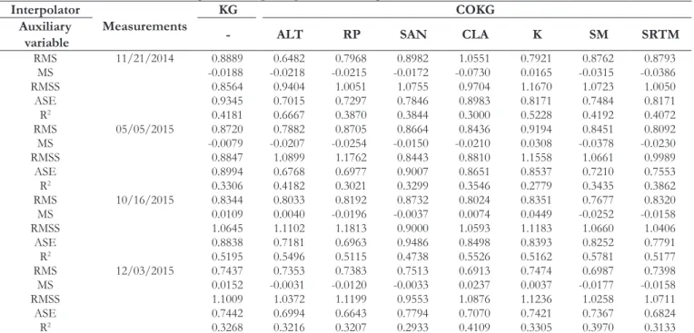
Cross validation
To analyze the interpolation quality, the values of ASE, RMSS, and R2 were considered determinant in the cross validation evaluation (Table 4).
Analysis of the resulting ASEs verified that most of the auxiliary variables were efficient by decreasing the error to a value
lower than that found using kriging. For the measurements made on 11/21/2014, 05/05/15, and 10/16/2015, all variables were
efficient with alternation in the granulometry values (SAN and CLA).
For the interpolation of the measurements made on 12/03/2015, only ALT, RP, CLA, and SRTM were able to reduce the ASE. The RMSS was considered adequate, although it varied above or below the ideal limit (should be close to 1), possibly contributing
to the increased error in some predictions or influencing the
lower error reduction. The R2 verification showed punctuated improvement in the predictions. However, the prediction model
showed moderate to low accuracy, reflecting the level of dependence
between the measured and predicted values.
Table 3. Variographic parameters.
Interpolator
Measurements
KG COKG
Auxiliary
Variable - ALT RP SAN CLA K SM SRTM
Model 11/21/2014 GAU. EXP EXP SPH GAU CIR EXP EXP a 661.50 2,771.40 2,983.90 2,836.60 794.00 816.50 1,792.00 2,788.30
C0 0.10 0.00 0.00 0.20 0.12 0.00 0.00 0.20
C 1.68 1.92 2.01 2.14 1.95 1.76 1.66 1.81
Model 05/05/2015 GAU EXP SPH SPH SPH SPH EXP EXP a 660.00 2,779.40 1,962.70 961.00 1,014.70 735.00 1,700.00 2,372.00
C0 0.08 0.00 0.14 0.00 0.00 0.00 0.00 0.05
C 1.57 1.64 1.34 1.62 1.67 1.40 1.36 1.60
Model 10/16/2015 GAU EXP CIR EXP GAU GAU GAU EXP a 784.40 3,354.00 1,724.5 2,917.60 964.00 792.00 950.00 3,044.00
C0 0.10 0.00 0.05 0.40 0.13 0.10 0.13 0.08
C 2.21 2.3 1.98 1.84 2.53 2.21 2.4 2.14
Model 12/03/2015 GAU EXP CIR EXP GAU GAU GAU EXP a 799.70 3,037.00 1,600.00 2,990.00 1,084.00 850.00 869.00 3,553.10
C0 0.13 0.20 0.15 0.35 0.16 0.13 0.15 0.20
C 1.31 1.11 1.15 1.03 1.50 1.44 1.34 1.15
ALT: altimetry of the topographic map; RP: resistance to penetration; SAN: percentage of sand; CLA: percentage of clay; K: hydraulic conductivity; SM: soil moisture; SRTM: altimetry of the SRTM product; a: range (m); C0: nugget effect; C: sill; EXP: exponential; CIR: circular; SPH: spherical; GAU: Gaussian; KG: kriging; COKG: cokriging.
Table 4. Cross validation for the interpolations regarding water table depths (m).
Interpolator
Measurements
KG COKG
Auxiliary
variable - ALT RP SAN CLA K SM SRTM
RMS 11/21/2014 0.8889 0.6482 0.7968 0.8982 1.0551 0.7921 0.8762 0.8793 MS -0.0188 -0.0218 -0.0215 -0.0172 -0.0730 0.0165 -0.0315 -0.0386 RMSS 0.8564 0.9404 1.0051 1.0755 0.9704 1.1670 1.0723 1.0050 ASE 0.9345 0.7015 0.7297 0.7846 0.8983 0.8171 0.7484 0.8171 R2 0.4181 0.6667 0.3870 0.3844 0.3000 0.5228 0.4192 0.4072
RMS 05/05/2015 0.8720 0.7882 0.8705 0.8664 0.8436 0.9194 0.8451 0.8092 MS -0.0079 -0.0207 -0.0254 -0.0150 -0.0210 0.0308 -0.0378 -0.0230 RMSS 0.8847 1.0899 1.1762 0.8443 0.8810 1.1558 1.0661 0.9989 ASE 0.8994 0.6768 0.6977 0.9007 0.8651 0.8537 0.7210 0.7553 R2 0.3306 0.4182 0.3021 0.3299 0.3546 0.2779 0.3435 0.3862
RMS 10/16/2015 0.8344 0.8033 0.8192 0.8732 0.8024 0.8351 0.7677 0.8320 MS 0.0109 0.0040 -0.0196 -0.0037 0.0074 0.0449 -0.0252 -0.0158 RMSS 1.0645 1.1102 1.1813 0.9000 1.0593 1.1183 1.0660 1.0406 ASE 0.8838 0.7181 0.6963 0.9486 0.8498 0.8393 0.8252 0.7791 R2 0.5195 0.5496 0.5115 0.4738 0.5526 0.5162 0.5781 0.5177
RMS 12/03/2015 0.7437 0.7353 0.7383 0.7513 0.6913 0.7474 0.6987 0.7398 MS 0.0152 -0.0031 -0.0120 -0.0033 0.0237 0.0037 -0.0177 -0.0158 RMSS 1.1009 1.0372 1.1199 0.9553 1.0876 1.1236 1.0258 1.0711 ASE 0.7442 0.6994 0.6643 0.7794 0.7070 0.7421 0.7367 0.6824 R2 0.3268 0.3216 0.3207 0.2933 0.4109 0.3305 0.3970 0.3133 MS: Mean Standardized; RMSS: Root Mean Square Standardized; ASE: Average Standard Error; RMS: Root Mean Square; R2: coefficient of determination; ALT: altimetry
Another way to verify the quality of the interpolations was to use maps incorporating the standard error of the interpolation (Figure 5), which made it possible to identify the best interpolations by cross-referencing with previously analyzed information. Therefore, it was possible to observe that the auxiliary variables ALT, RP, and SRTM gave the most consistent results in the interpolated measurements.
This differential behavior of the auxiliary variables in the results is because each soil property used presents different spatial variability behavior, necessitating different strategies of obtaining data for each auxiliary variable. Another fact considered is the variability in each of the methods of obtaining the values of the physical hydric properties of the soil.
The difference found between the measurements of the water table depth reveals the difference in the behavior of the
fluctuation of the water level in each well under the influence of
climatic dynamics and the characteristics of the aquifer. Another phenomenon that caused behavioral change in the parameters of the spatial prediction was the difference in the way the sample set related to each auxiliary variable.
In undisturbed groundwater systems, climatological conditions can be considered the only factor. This approach can be considered in the interpretation of the spatial variation of groundwater dynamics, because spatial differences in groundwater dynamics are determined by the spatial variation of the system properties, while the temporal variation is driven by the dynamics of the input into the system (VON ASMUTH; KNOTTERS, 2004).
The maps generated using cokriging and ALT were used to calculate the volumes recovered in the analyzed period. Using topographic data as auxiliary variables for the interpolation of water table depths, Rocha et al. (2009) also achieved better geostatistical modeling. By incorporating topographic data in the spatial analysis of groundwater, they observed an important decrease in the sample variation marked by the reduction of the variogram sill.
The results show that the application of the auxiliary variables and data fusion from different scales in groundwater mapping can favor and improve of the quality of the information provide for water management. It also could replicated similar
environmental conditions to those found in the field trips at
EEcSB, providing information to explore the seasonal variation of the water volume in areas with an imminent or permanent situation of water resources scarcity.
Extractable water volume
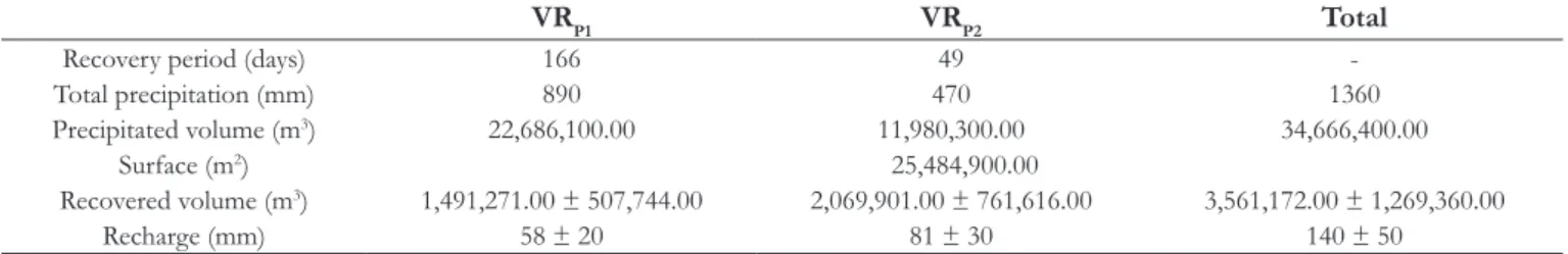
The best maps were selected (Figures 6 and 7) to calculate the volume of water that was recovered in studied periods P1 and P2. Using this methodology, calculated the volumes of recovered water (VR) for each of the two periods (VRP1 and VRP2). The recharge volume was calculated according to the use of Equation 5 and compared to the volume precipitated in the period. The total height of precipitation responsible for level recovery was 890 mm for VRP1 and 470 mm for VRP2 (total: 1360 mm). This value, converted to a volume relative to the surface of the evaluated basins (2549 hectares), represents a precipitated volume of 34,666,400.00 m3.
Figure 6. Oscillation of water table depth in studied periods P1.
Thus, the total recovered value is equivalent to 10% of the rainfall and it represents a recharge of 140 mm (Table 5).
Comparison of both recovery periods shows that rainfall was more widely distributed but with lower recharge in VRP1, whereas in VRP2, rainfall was more concentrated, resulting in greater recharge in a shorter period. It is possible to infer that the volume to be collected depends directly on precipitation behavior, because water table depth oscillation is very susceptible to precipitation events.
The average water consumption in the municipalities of Águas de Santa Barbara, Manduri, and Cerqueira Cesar, according to data from the National System of Information on Sanitation, is shown in Table 6. An evaluation of the calculated values based on the collection of 30% of the VR in the EEcSB basins is presented in Table 7. This volume would be sufficient to supply water to the municipalities for three months, even when considering a 20% loss in the water catchment and distribution system. It is only a simulation for the use of the seasonal oscillation of groundwater.
Average uncertainties were incorporated to the spatial prediction model in the extractable water volume calculations to measure the effects of the ASE in the method application. The considered variation refers to minimal deviation close to the monitoring wells, in the region where water table depth data collection are concentrated, since the uncertainty in areas where the prediction was extrapolated generates a higher variation than
the natural oscillation verified in VRP1 and VRP2. This behavior
exposes a limitation in the methodology application. Thus, it is necessary to undertake new experiments to test sampling
configurations, because sampling optimization can reduce the
uncertainties reducing the variance and minimizing errors, providing more accurate estimates for water resources management.
CONCLUSIONS
This study examined the efficacy of using different physical
hydric variables of soils and topography as auxiliary depths in forest areas, based on geostatistical interpolation, and producing important information for the advancement of spatial data studies. The use of such information produced satisfactory results in the interpolation of water table depths, especially in cases when RP, ALT, and SRTM were used as secondary variables.
The use of cokriging as an interpolator gave superior results in comparison with those achieved by kriging alone, as seen from the variographic parameters in the cross validation and in the standard error maps. However, the uncertainty present in the spatial prediction exposes the limitation of the method. Thus, adaptations are required to promote changes in data collection to reduce uncertainties and to provide estimates that are more accurate for the management of water resources.
The generated maps constitute an important tool for the management of water resources in priority areas, where aquifers are particularly vulnerable both to anthropic factors and to the effects of climate change. Understanding the dynamics of water table depth oscillation might facilitate faster response in times of water scarcity, alleviating the impacts on society by including strategic reserves of short-term groundwater volumes during times of pronounced drought, as seen in 2014.
Table 5. Stored volumes of precipitation in the aquifer during the rainy season between November 2014 and December 2015.
VRP1 VRP2 Total
Recovery period (days) 166 49
-Total precipitation (mm) 890 470 1360
Precipitated volume (m3) 22,686,100.00 11,980,300.00 34,666,400.00
Surface (m2) 25,484,900.00
Recovered volume (m3) 1,491,271.00 ± 507,744.00 2,069,901.00 ± 761,616.00 3,561,172.00 ± 1,269,360.00
Recharge (mm) 58 ± 20 81 ± 30 140 ± 50
Table 6. Water volume for the monthly supply of cities near the Santa Barbara Ecological Station.
Municipalities
Average consumption
per capita (l/day)
Population (inh.)
Monthly consumption
(m3)
Águas de Santa Barbara 201 5,600 33,768.00
Manduri 277 8,900 73,959.00
Cerqueira Cesar 222 17,530 116,750.00
Total - 32,030 224,477.00
Table 7. Extractable volume (m3) and months of water supply.
Extractable volume (m3) Months of
water supply
ACKNOWLEDGEMENTS
The authors are grateful to FAPESP (São Paulo Foundation
for Scientific Research) for funding (Grants 2014/04524-7 and
2016/09737-4) and master scholarship (Grant 2015/05171-3), and to Instituto Florestal (IF) do Estado de São Paulo and LabH2O/UNESP/Ourinhos team members involved in this
study for field support.
REFERENCES
AHMADI, S. H.; SEDGHAMIZ, A. Application and evaluation of kriging and cokriging methods on groundwater depth mapping. Environmental Monitoring and Assessment, v. 138, n. 1-3, p. 357-368, 2008. http://dx.doi.org/10.1007/s10661-007-9803-2. PMid:17525831.
BAALOUSHA, H. Assessment of a groundwater quality monitoring network using vulnerability mapping and geostatistics: a case study from Heretaunga Plains, New Zealand. Agricultural Water Management, v. 97, n. 2, p. 240-246, 2010. http://dx.doi. org/10.1016/j.agwat.2009.09.013.
BETTÚ, D. F.; FERREIRA, F. J. F. Modelos da superfície potenciométrica do Sistema Aqüífero Caiuá no noroeste do estado do Paraná: comparação entre krigagem ordinária e krigagem com tendência externa do modelo numérico do terreno. Águas Subterrâneas, v. 19, n. 2, p. 55-66, 2005.
CAO, G.; YOO, E.; WANG, S. A statistical framework of data fusion for spatial prediction of categorical variables. Stochastic Environmental Research and Risk Assessment, v. 28, n. 7, p. 1785-1799, 2014. http://dx.doi.org/10.1007/s00477-013-0842-7.
DESBARATS, A. J.; LOGAN, C. E.; HINTON, M. J.; SHARPE, D. R. On the kriging of water table elevations using collateral information from a digital elevation model. Journal of Hydrology, v. 255, n. 1-4, p. 25-38, 2002. http://dx.doi.org/10.1016/S0022-1694(01)00504-2.
DILLON, P.; SIMMERS, I. (Eds.). Shallow groundwater systems. Balkema: Rotterdam, 1998.
FETTER, C. W. (Ed.). Applied hydrogeology. 4th ed. Upper Saddle River: Prentice Hall, 2001.
GOOVAERTS, P. (Ed.). Geostatistics for natural resources evaluation. New York: Oxford University Press, 1997.
HENGL, T. (Ed.). A practical guide to geostatistical mapping. 2nd ed. Amsterdam: Hengl, 2009.
HOOSHMAND, A.; DELGHANDI, M.; IZADI, A.; AALI, K. A. Application of kriging and cokriging in spatial estimation of groundwater quality parameters. African Journal of Agricultural Research, v. 6, n. 14, p. 3402-3408, 2011.
ISAAKS, E. H.; SRIVASTAVA, R. M. (Eds.). Applied geostatistics. New York: Oxford University Press, 1989.
JOHNSTON, K.; KRIVORUCHKO, K.; LUCAS, N.; VER HOEF, J. M. (Eds.). Using ArcGIS geostatistical analyst. Redlands: ESRI, 2001. KAMBHAMMETTU, B. V. N. P.; ALLENA, P.; KING, J. P. Application and evaluation of universal kriging for optimal contouring of groundwater levels. Journal of Earth System Science, v. 120, n. 3, p. 413-422, 2011. http://dx.doi.org/10.1007/s12040-011-0075-4.
KITANIDIS, P. K. (Ed.). Introduction to geostatistics: applications to hydrogeology. Cambridge; New York: Cambridge University Press, 1997. http://dx.doi.org/10.1017/CBO9780511626166.
KNOTTERS, M.; BIERKENS, M. F. Predicting water table depths in space and time using a regionalised time series model. Geoderma, v. 103, n. 1, p. 51-77, 2001. http://dx.doi.org/10.1016/ S0016-7061(01)00069-6.
KRESIC, N.; MIKSZEWSKI, A. (Eds.). Hydrogeological conceptual site models: data analysis and visualization. Boca Raton: CRC Press, 2013. MANZIONE, R. L.; DRUCK, S.; CÂMARA, G.; MONTEIRO, A. M. V. Modelagem de incertezas na análise espaço-temporal dos níveis freáticos em uma bacia hidrográfica. Pesquisa Agropecuária Brasileira, v. 42, n. 1, p. 25-34, 2007. http://dx.doi.org/10.1590/ S0100-204X2007000100004.
MANZIONE, R. L.; MARCUZZO, F. F. N.; WENDLAND, E. C. Integração de modelos espaciais e temporais para predições de níveis freáticos extremos. Pesquisa Agropecuária Brasileira, v. 47, n. 9, p. 1368-1375, 2012. http://dx.doi.org/10.1590/S0100-204X2012000900022.
NGUYEN, H.; CRESSIE, N.; BRAVERMAN, A. Spatial statistical data fusion for remote sensing applications. Journal of the American Statistical Association, v. 107, n. 499, p. 1004-1018, 2012. http:// dx.doi.org/10.1080/01621459.2012.694717.
PETERSON, T. J.; CHENG, X.; WESTERN, A. W.; SIRIWARDENA, L.; WEALANDS, S. R. Novel indicator geostatistics for water table mapping that incorporate elevation, land use, stream network and physical constraints to provide probabilistic estimation of heads and fluxes. In: INTERNATIONAL CONGRESS ON
MODELLING AND SIMULATION, 19., 2011, Perth. Anais…
Australia: Modelling and Simulation Society of Australia and New Zealand, 2011. Disponível em: <http://www.mssanz.org. au.previewdns.com/modsim2011/I9/peterson.pdf> Acesso em: 11 nov. 2015.
ROCHA, M. M.; YAMAMOTO, J. K.; FONTELES, H. R. N. Cokrigagem ordinária versus krigagem com deriva externa: aplicações para a avaliação do nível potenciométrico em um aquífero livre.
Geologia USP Série Científica, v. 9, n. 1, p. 73-84, 2009. http://dx.doi. org/10.5327/Z1519-874X2009000100005.
Faculdade de Ciências Agronômicas, Botucatu, 2016. Disponível em:<http://hdl.handle.net/11449/143849>. Acesso em: 1 dez. 2016.
SOARES, A. (Ed.). Geoestatística para as ciências da terra e do ambiente. 2nd ed. Lisboa: IST Press, 2006.
VON ASMUTH, J. R.; KNOTTERS, M. Characterising groundwater dynamics based on a system identification approach. Journal of Hydrology, v. 296, n. 1-4, p. 118-134, 2004. http://dx.doi. org/10.1016/j.jhydrol.2004.03.015.
YAMAMOTO, J. K.; LANDIM, P. M. B. Geoestatística: conceitos e aplicações. São Paulo: Oficina de Textos, 2015.
Authors contributions
Lucas Vituri Santarosa: Field implementation of water table depths monitoring network, sampling and data collection, data modelling, results analysis and manuscript preparation including
writing, figures and tables preparation, bibliographical revision
and translation to English language.
Rodrigo Lilla Manzione: Experimental design, field implementation