Validation of the method used by the SUBER model for the estimation of
extracted cork dry weight with more and less than 9 years of growth
Marta Felip Ruiz
Dissertation for the Master's Degree
Mediterranean Forestry and Natural Resources Management (MEDfOR)
Tutors: Joana Amaral Paulo
Margarida Tomé
Jury:
President: Dr. Maria Helena Reis de Noronha Ribeiro de Almeida, Associate professor at Instituto Superior de Agronomia in University of Lisbon
Vowel: Dr. Maria Augusta Fernandes Pereira da Costa de Sousa, Assistant researcher at Instituto Nacional de Investigação Agrária e Veterinária.
Vowel: Dr. Joana Amaral Paulo, Post-doctoral fellowship from Fundação para a Ciência e a Tecnologia
Vowel: Dr. Vanda Cristina Paiva Tavares de Oliveira, Post-doctoral fellowship from Fundação para a Ciência e a Tecnologia
ACKNOWLEDGMENTS
To all my family and friends that have been supporting me and cheering me up during the hole process of the writing and defense of this thesis.
To the Forchange group (Forest Ecosystem Management under Global Change), investigation group of the Centro de Estudos Florestais in Instituto Superior de Agronomia that helped me in several parts of the thesis and let me participate in some field work for their projects that I really enjoyed it.
Especially to Joana Amaral Paulo (tutor) for the attention and carefulness that she put on the work and the facilitations that she gave to me in order to finish in time, thanks.
Also to Paulo Firmino, that helped me with the samples and all the practical stuff and, above all, for his moral support and kindness.
Thanks to Catarina Tavares and Ágata Lam for all their help in the administrative procedures even when they didn’t have to.
RESUMO (Portuguese)
A extração de cortiça constitui uma das principais atividades dos montados de sobro em Portugal, país onde está presente em 23% da área florestal. Portugal e Espanha em conjunto são responsáveis pela produção de 80% da cortiça a nível mundial.
A camada de cortiça é originada pela atividade contínua do felogénio, o qual morre e regenera após a operação de descortiçamento permitindo a formação de uma nova camada de cortiça. Esta operação de descortiçamento ocorre geralmente a cada 9 anos (mínimo permitido pela legislação nacional). No entanto, existem frequentemente exceções. Em alguns casos, para situações definidas no decreto lei em vigor (DL 169/2001 e DL 155/2004), a extração pode ser efetuada com 7 ou 8 anos após pedido de autorização às entidades competentes. É o caso do acerto de diferentes anos de tiradas numa área de gestão. O descortiçamento pode também ser efetuado em intervalos maiores que 9 anos, por opção do gestor floresta, perante uma ou mais das seguintes situações:
i) decréscimo do preço da cortiça
ii) condições climáticas adversas no ano e/ou do novénio iii) mau estado vegetativo das árvores
iv) reduzido calibre da cortiça aos 9 anos
Atualmente, em Portugal, a cortiça é vendida por unidade de peso, sendo estabelecido em cada situação entre o vendedor e o comprador, um preço para o material a comercializar. A determinação do peso extraído de cortiça pode ser feita de diferentes maneiras:
i) na árvore por estimativa visual (método menos recomendado pelas associações de produtores)
ii) estimativa com base em modelos de predição do peso de cortiça que utilizam variáveis recolhidas em inventário (da árvore ou do povoamento)
iii) pesagem após o descortiçamento (em verde – cortiça pesada após a extração – ou após um periodo de secagem em pilha)
No que diz respeito ao conhecimento da qualidade da cortiça, determinada considerando calibre, porosidade e presença de defeitos da cortiça, apenas a amostragem prévia com a recolha de calas (método ii) permite efetuar a caracterização do material a extrair. Esta amostragem é efetuada por diversas associações de produtores, seguindo um desenho amostral definido por Almeida e Tomé (2008).
A maioria dos modelos que existem para a estimativa do peso de cortiça extraída (método ii) ao nível da árvore apenas consideram cortiças com 9 ou 10 anos de idade. Paulo e Tomé (2010) desenvolveram um método que
permite a estimativa do peso de cortiça extraída ao nível da árvore qualquer que seja a sua idade (t anos de crescimento). O método baseia-se no conhecimento existente de que a densidade da cortiça é constante entre os anéis de cortiça, sendo apenas significativamente diferente a densidade da costa da cortiça. O método é baseado na aplicação de dois sub-modelos: 1) modelo que prevê a biomassa de cortiça com 9 anos de idade utilizando um de entre quatro modelos alternativos (modelos I, II, III e IV); 2) modelo que estima a proporção de peso de costa de cortiça aos 9 anos de idade. Os valores obtidos por estes modelos permitem a estimativa do peso de cortiça, para qualquer que seja a sua idade de crescimento, através de um método descrito em Paulo e Tomé (2010). O método encontra-se validado apenas para 9, 10 e 11 anos de idade de cortiça, sendo que os objetivos deste trabalho foram levar a cabo a validação para as idades de 8 e 13 anos, e discutir alternativas para a melhoria dos modelos e das estimativas de produção de cortiça produzidas.
Para o trabalho de validação estavam disponíveis, ao nível da árvore individual, amostras de cortiça (calas), medições dendrométricas das árvores e pesos secos de cortiça. As amostras foram recolhidas em povoamentos distribuídos ao longo da região sudoeste de Portugal: Sacavém (14 calas), Fontanal (13 calas), Lantiscais (24 calas) e Fontainhas (109 calas), num total de 160 calas. Em Sacavém a cortiça tinha 8 anos de idade e nos restantes povoamentos tinha 13 anos. No âmbito deste trabalho estas amostras foram cozidas (processo de cozedura de acordo com o procedimento industrial habitual, a 100 ºC durante 1 hora, efetuado na Associação de Produtores Florestais de Coruche) e o calibre foi medido antes e depois da cozedura (calibre incluindo a barriga e a costa da cala).
O processo de validação implicou o cálculo dos valores estimados de peso de cortiça pelo método proposto por Paulo e Tomé (2010), e a posterior comparação destes com os valores observados (medidos) através do cálculo dos resíduos (valor observado – valor estimado). A validação foi efetuada considerando cada um dos 4 modelos disponíveis para determinação do peso de cortiça com 9 anos (modelos I, II, III e IV), por forma a avaliar a importância da utilização de modelos com variáveis referentes à intensidade de descortiçamento (modelos II e III) e de modelos com variáveis referentes ao calibre da cortiça da árvore (modelo IV), em alternativa a um modelo que apenas incluí a variável diâmetro à altura do peito (modelo I).
Os resíduos foram avaliados em termos de enviesamento e precisão, através do cálculo e da análise dos valores da média dos resíduos e da média dos valores absolutos dos resíduos, respetivamente. Também foram calculados os percentis de 5% e 95% dos resíduos e o valor da eficiência da modelação. A mesma análise foi feita aos valores dos resíduos expressos em termos percentuais do peso de cortiça extraído da árvore. Esta análise foi feita inicialmente para o conjunto total dos dados de validação, e de seguida para o conjunto de dados agrupados segundo as seguintes variáveis: idade da cortiça (8, 9, 10, 11 e 13 anos), diâmetro à altura do peito sem cortiça (classes de 5 cm
de amplitude), classes de espessura de cortiça segundo as definidas pela indústria (delgadinha, delgada, meia
marca, marca, grossa e triângulo), e número de pernadas de primeira ordem descortiçadas.
Os resultados do presente trabalho mostram que a utilização do modelo IV na fase de estimativa do peso de cortiça com 9 anos é a que resulta em estimativas com maior valor de precisão (média dos resíduos absolutos, em percentagem do peso de cortiça extraído da árvore, variando entre 8 e 25%) e menor enviesamento (média dos resíduos, em percentagem do peso de cortiça extraído da árvore, variando entre -7 e 23%) das estimativas finais. Este modelo, incluindo variáveis da árvore e da cortiça, exige não só a realização de inventário florestal, mas também a realização de uma amostragem à cortiça antes do descortiçamento, na qual seja medido diretamente na árvore o calibre, ou retirada uma amostra de cortiça (cala) para medição em gabinete. Por outro lado o modelo I, dependente apenas da variável diâmetro da árvore, embora menos exigente no que diz respeito a recolha de dados, resulta em estimativas menos exatas: precisão (média dos resíduos absolutos, em percentagem do peso de cortiça extraído da árvore) entre 23 e 46%, e enviesamento (média dos resíduos, em percentagem do peso de cortiça extraído da árvore) entre -32 e 36%. Os modelos II e III apresentam resultados intermédios.
A validação do método permitiu ainda concluir:
1. É possível estimar a produção da biomassa de cortiça com valores de eficiência de modelação entre 0,12 e 0,99, com uma média de 0,80, a partir das características dendrométricas da árvore e da cortiça incluídas como preditoras no modelo
2. Para as seguintes situações todos os modelos de previsão de cortiça são positivamente enviesados (predizem valores de biomassa de cortiça inferiores aos observados):
- idade da cortiça superior a 11 anos - classes de diâmetros superiores a 40 cm
- classes de espessura de cortiça das classes grossa e triângulo
3. O enviesamento diminui quando os modelos incluem mais variáveis como preditores (ao passar da utilização do modelo I para o II, III ou IV)
4. O enviesamento ocorre principalmente para as classes extremas, por exemplo, cortiças das classes
delgadinha e triângulo
5. A medição da altura vertical de descortiçamento diminui o enviesamento e aumenta a precisão na previsão da biomassa da cortiça. Por exemplo, para cortiças com 8 anos, o enviesamento (média dos resíduos, em percentagem do peso de cortiça extraído da árvore) das estimativas reduz-se de -26 para 0,8% e a precisão (média dos resíduos absolutos, em percentagem do peso de cortiça extraído da árvore) aumenta de 43 para 26% com a utilização do modelo III em alternativa ao modelo II
6. A medição da espessura da cortiça e utilização do modelo IV permite diminuir o erro na predição, em particular para cortiças das classes delgadinha e triângulo (passando do modelo III para o IV o enviesamento reduz-se de -28 para -7% em delgadinha e 34 para 23% em triângulo; e a precisão aumenta de 30 para 20% em delgadinha e 34 para 25% em triângulo)
Os resultados obtidos permitem propor a melhoria dos modelos de determinação do peso de cortiça como forma de melhorar a estimativa do peso de cortiça extraída, nomeadamente através do seu reajustamento com um maior número de observações respeitantes ao peso de cortiça extraída nos casos de árvores produtoras de cortiças muito finas e muito grossas. Outra alternativa que se coloca é a comparação deste método com outro baseado apenas numa equação preditora do peso de cortiça, que inclua a variável idade da cortiça como variável independente. Esta alternativa implicaria o investimento de tempo e recursos na recolha de mais observações referentes a peso de cortiça extraída em casos de idades de cortiça igual a 12 e superior a 13 anos.
ABSTRACT (English)
Extraction of cork from montados or cork oak forests is one of the main activities in Portugal. 23% of Portuguese forests are from Quercus suber and Portugal is the main producer of cork in the world. Commonly, every 9 years, but also 10 or more, the cork of the stem and branches with perimeter at breast height greater than 70 cm is removed. Possibly this intervals are not the optimum for the production of cork. Most of the models that exist only predict cork weight for 9 or 10 years of cork age. But a new model developed by Paulo and Tomé (2010) allows the prediction of mature cork biomass with t years of growth, based in one measurement taken at any other age. The model is based on two sub-models; the first one predicts cork biomass with 9 years of age using four alternative models with different variables as inputs; and a second one that estimates cork back weight proportion at 9 years of age. The method has already been validated for 9, 10 and 11 years of cork age, and the objective of this work was doing the validation of the model for that ages and also adding new data of 8 and 13 years of cork age. The evaluation was done by comparing the observed and the estimated values of cork biomass from corks with 8, 9, 10, 11 and 13 years of age. According to previous validation, it was confirmed that the model work better as more input variables are added in the model and it was also found that as the ages of cork biomass move away from 9 years, as well as the extremes of cork thickness classes, the worst is the performance of the model.
CONTENT
LIST OF FIGURES ... 1 LIST OF TABLES ... 3 1. INTRODUCTION ... 4 2. DATA ... 6 2.1. MEASUREMENTS ... 7 3. METHODS ... 113.1. Models for predicting cork biomass with 9 years of age (wcm9) ... 12
3.2. Predicting cork bark weight proportion at 9 years of age (cbp9) ... 14
3.3. Validation of the Paulo and Tomé (2010) method ... 14
4. RESULTS ... 18
4.1. Results according to cork age ... 20
4.2. Results according to diameter under cork ... 23
4.3. Results according to cork thickness classes ... 27
4.4. Results according to the number of first-order debarked branches ... 30
4.5. General results ... 34
5. DISCUSSION ... 36
6. CONCLUSION ... 38
1
LIST OF FIGURES
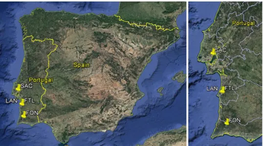
Figure 1: Location of the sites where data were collected. The labels LAN, FTL, FON and SAC correspond to
Lantiscais, Fontanal, Fontainhas and Sacavém respectively. Source: Google earth. ... 6
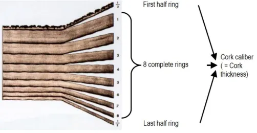
Figure 2: Schematic representation of a cork sample with 9 years, showing the 8 complete cork rings and the 2 half rings (Adapted from Natividade (1950) and Almeida et al. (2010)). ... 8
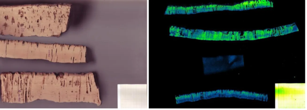
Figure 3: Examples of scans of some “calas”. Without filters (left) and with filters (right). ... 9
Figure 4: Relationship between mature cork biomass and diameter under bark at breast height: x, cork with 13 years (left) and ◊, with 8 years (right). ... 9
Figure 5: Procedure by steps of the transformations by equations of the data, from cork caliber at t years to cork caliber at 9 years of age. ... 13
Figure 6: Schematic representation of bias and precision terms (Vanclay, 1994). ... 15
Figure 7: Relationship between cork thickness after and before boiling in mm: x, cork with 13 years (left) and ◊, with 8 years (right). ... 18
Figure 8: Relationship between cork thicknesses after boiling measured directly and estimated by Almeida and Tomé (2008) system of equations in mm: x, cork with 13 years (left) and ◊, with 8 years (right). ... 19
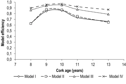
Figure 9: Model efficiency along 8, 9, 10, 11 and 13 years of cork ages for the different models tested. ... 20
Figure 10: Bias of the tested models with cork age – mean value of the residuals (kg). ... 21
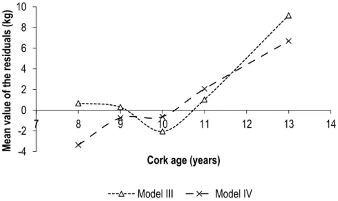
Figure 11: Bias of model III and IV with cork age – mean value of the residuals (kg). ... 21
Figure 12: Bias of the tested models with cork age – mean of value of the residuals (%). ... 22
Figure 13: Precision of the tested models with cork age – mean of absolute value of the residuals (%). ... 23
Figure 14: Model efficiency for diameter under cork classes (cm) for the different tested models. ... 24
2
Figure 16: Bias of the tested models with diameter under the cork – mean of value of the residuals (%). ... 26
Figure 17: Precision of the tested models with diameter under the cork – mean of absolute value of the residuals (%). ... 26
Figure 18: Model efficiency for cork thickness classes for the different tested models. ... 28
Figure 19: Bias of the tested models with cork thicknesses classes – mean value of the residuals (kg). ... 28
Figure 20: Bias of the tested models with cork thicknesses classes – mean value of the residuals (%). ... 29
Figure 21: Precision of the tested models with cork thickness classes – mean of absolute value of the residuals (%). ... 29
Figure 22: Model efficiency for number of debarked branches for the different tested models. ... 31
Figure 23: Bias of the tested models with number of debarked branches – mean value of the residuals (kg). ... 32
Figure 24: Bias of the tested models with number of debarked branches – mean value of the residuals (%). ... 32
Figure 25: Precision of the tested models with number of debarked branches – mean of absolute value of the residuals (%). ... 33
Figure 26: Relationship of average value for 8 complete years cork thickness (mm) and by 5 cm range tree diameter under cork classes (cm). ... 34
3
LIST OF TABLES
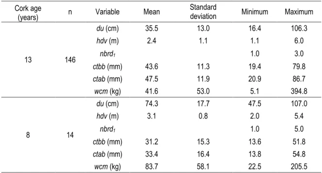
Table 1: Summary statistics of the variables for 13 and 8 years of cork age. ... 10
Table 2: Models for cork biomass prediction for 9 years of age (Paulo and Tomé, 2010). ... 12
Table 3: System of equations from Almeida and Tomé (2008) used for the estimation of the 9 years cork thickness value after boiling, used as an independent variable in Paulo and Tomé (2010) model IV ... 13
Table 4: Validation statistics obtained for the Paulo and Tomé (2010) method, considering together as a validation data set the samples collected for this thesis (8 and 13 years old cork) and the ones used by Paulo and Tomé (2010) (9, 10 and 11 years old cork). Statistics are presented separately considering the usage of alternative models I, II, III and IV for the estimation of cork biomass with 9 years old (see section 3 for details). ... 19
Table 5: Frequency distribution for cork age (years). ... 20
Table 6: Frequency distribution for diameter under cork classes (cm). ... 24
Table 7: Frequency distribution and intervals (in mm) for cork thickness classes. ... 27
1. Introduction
4
1.
INTRODUCTION
The montado or cork oak forests cover a worldwide area of 2,139,942 hectares. Cork oak is a typical species of the Western Mediterranean region, occurring spontaneously in Portugal and Spain, but also in Morocco, in Northern Algeria and Tunisia (Pereira and Tomé, 2004). It appears mainly in pure cork oak forests and cork oak based agro-forestry systems. In addition, it is found in more restricted areas in the south of France and on the west coast of Italy, including Sicily, Corsica and Sardinia. Portugal has 34% of the world’s area, which corresponds to an area of 736,775 thousand hectares and 23% of national forest (IFN6, 2013). Portugal and Spain have the clear leadership in terms of areas of cork oak forests representing, together, more than three quarters of the world’s cork production, 49.6% and 30.5% respectively. In year 2010 world cork production rose to 201,428 tons per year. Portugal continues to be the leader, with an average annual production of more than 100 thousand tons per year. The main target of the cork products are the bottle stoppers for wine which accounts for 72% of what is produced, followed by the construction sector with 28% (APCOR, 2016).
The cork layer is originated by the continuous activity of the phellogen. Periodically (commonly at 9-year intervals, but also 10 or more), the cork of the stem and branches of trees with perimeter at breast height greater than 70 cm is removed through the debarking operation. The phellogen dies in the debarking operation but a new phellogen layer is regenerated inside the inactive phloem, allowing the formation of a new cork layer. The extracted cork planks are then the raw material for cork stoppers and other less valuable cork products as agglomerates.
Models for assessing, in a quantitative way, the production of non-timber products in different forest situations and for different management schedules are required (Calama et al., 2010). The importance of cork production makes the development of cork biomass prediction models a necessary tool for two different scenarios: (1) for the forest management, where cork biomass models are tools to develop integrated management models as important as diameter, cork growth and cork quality models and (2) for the economy, allowing the assessment of cork production at local, regional and national level allows a better programming for the industry supply of raw material and the exportation of manufactured products (Vázquez and Pereira, 2005).
Currently in Portugal the cork is sold per unit of weight. In some farms, previously to the debarking operation, an estimation of cork production, quality and average cork price is carried out. This estimation is extremely important to forest landowners for cork commercialisation and it needs to be as accurate as possible to the reality. Currently the cork sampling methodology with a more efficient precision/cost ratio is used and arises from the method proposed by Almeida and Tomé (2010).
1. Introduction
5 The complexity and dynamism of the forest systems make difficult the prediction of the system behaviour. Forest systems are subjected to many external and internal factors that are not yet completely understood. The climatic and microclimatic factors, the availability of nutrients and water, the interaction between and within species, the intrinsic characteristics of each species make really complex the knowledge of what factor influences each characteristic, and also the combination of them causes distinct responses. In this case, use of models helps us to find easily the nature response with the introduction of several parameters measured in the field and in the lab.
Forest modelling rises from the need of the managers to quantify the forest on the long term as a support to their decisions. The variables that we use to characterize the forests such as tree and stand dimension, production, growth, etc. are difficult, expensive and time consuming to achieve; for that reason, it is common the use of models to get information of variables like those. The models allow the user to get information of the development of the stand, the production of cork and wood, economic sustainability and carbon sequestration. Those are useful tools for the sustainable management of cork oak stands, used for stand characterisation, the definition of management areas, simulation of the stand evolution, definition of forest management plans and research.
Growth and production models allow forest managers to evaluate the consequences of the different management alternatives and strategies, in processes that can be from periodic growth of trees to succession of the species in the forest (Vanclay and Skovsgaard, 1996). In practice, process-based models (e.g., Mäkela et al., 2000) have been used when modelling is undertaken for the purpose of understanding, while growth and yield models (e.g., Vuokila, 1965; Shao and Reynolds, 2006) are widely used when the objective is prediction (Burkhart and Tomé, 2012).
For this study the focus was on the cork production module of the SUBER model (described in Paulo, 2011), an empirical model, more specifically a growth and production model, implemented in the sIMfLOR platform (Faias, 2012). It can also be classified inside the category of individual tree, distance independent growth model (Munro, 1974; Burkhart et al., 1981; Monserud, 2003). The objective of the present study was validating the cork biomass module for the estimation of extracted mature cork biomass with more or less than 9 years of cork growth, and to discuss alternatives for the improvement of the estimates. The first validation has been presented by Paulo and Tomé (2010) for cork with 9, 10 and 11 years of growth; this study was focused on trees with cork older than 11 years and younger than 9. The results of the study should be really interesting for landowners, managers and for the cork industry in general as a predictable tool for quantifying the cork of the stands. Also the results should be relevant for the study of the differences of biomass in variable rotation periods in order to know when it is better to do the debarking operation as a decision tool. If this model can be valid for any t years of growth, the cork producers could be more efficient in decision making procedure and for future predictions.
2. Data
6
2.
DATA
Data used for the validation procedure was collected in four distinct sites distributed along the south west of Portugal: Sacavém, Fontanal, Lantiscais and Fontainhas (Figure 1). The trees were debarked in 2009 in Sacavém and 2010 in the other sites. The distribution of the samples was the following:
24 tree samples from Lantiscais (Alentejo, Setúbal), reference LAN, collected in 2010. UTM 29S 519151 4201549
13 tree samples from Fontanal (Alentejo, Setúbal), reference FTL, collected in 2010. UTM 29S 520905 4202699
109 tree samples from Fontainhas (Algarve, Faro), reference FON, collected in 2010. UTM 29S 535423 4124650
14 tree samples from Sacavém (Loures, Lisboa), reference SAC, collected in 2009. UTM 29S 491571 4294566
Figure 1: Location of the sites where data were collected. The labels LAN, FTL, FON and SAC correspond to Lantiscais, Fontanal, Fontainhas and Sacavém respectively. Source: Google earth.
Also, the data used for validation from Paulo and Tomé (2010) was used; the results from both works were joined and resulted in the final validation data set. The data corresponding to their work were: 100 samples for 9 years cork, 90 samples for 10 years cork and 93 samples for 11 years cork. In total 443 samples were used for validation purposes.
2. Data
7 2.1. MEASUREMENTS
The total extracted cork from each tree was weighted immediately after cork extraction, together with a sample taken at breast height (20 cm x 20 cm, called cala) that was used to determine the cork humidity in the laboratory, and consequently the mature cork biomass. A second sample, also taken at breast height and with the same dimensions, was used for cork thickness measurements, both before and after boiling (ctbb and ctab). For the determination of the dry weight the samples were dried until stabilization of the weight.
After extraction from the tree, the cork planks usually undergo a postharvest preparation for further industrial processing consisting of an immersion in water at approximately boiling temperature during 1 h. The objective of this operation is to flatten the raw planks, curved according to the stem shape, to clean them, extract the water-soluble substances from them, improve their smoothness and elasticity, and to soften the cork tissue for an easier subsequent cutting; also a consequence is a density decrease. With water boiling the cork expands and the most important practical consequence is that the raw cork planks increase in thickness, on average 12% (Pereira and Tomé, 2004). This operation also ensures that the microflora is significantly reduced (APCOR, 2006). Additionally, cork thickness after boiling best represents the real cork thickness considered for industrial purposes. Since it is measured after the internal tensions, caused by the cellular corrugation during cork growth occurring between the wood and the external cork layers, have been relieved during the water boiling of cork (Pereira, 2007).
During the sampling, tree dendrometric variables have been measured to be used as repressors variables in the models. The diameter at breast height under bark is one of the most common, simple and cheap measurement that is taken in an inventory. It was measured easily with a tape and can provide information of tree size. The second one was the total height that can be useful in other studies but not really in the present work. The interesting height here was the total and vertical debarked height that can provide information on the quantity of debarked cork and the intensity of the debarking process, although it is not commonly registered in the inventories. The last variable measured was the number of debarked branches that was easily taken by naked eye and useful in order to predict cork quantity and also a measure of the debarking intensity.
The thickness of the cork plank, or cork caliber according to the industry terminology, is the most important variable when analysing the raw material suitability for the production of stoppers (Pereira and Tomé, 2004). In this work the term cork thickness was used with the same meaning to cork caliber and if it is not specified it is always after boiling. Also another term that was used is the thickness of complete rings that discounts from the cork caliber the first and the last half rings/years and the cork back. The cork is extracted during the growing season, starting the growth of the new cork shortly after the extraction. The first growth ring is therefore an incomplete ring, many times including cork
2. Data
8 and dead phelogen tissues (usually called costa or cork back), and in the opposite way, the last ring is also incomplete. The scheme of Figure 2 shows the differences between these two thicknesses. The thickness of the cork is the main cause of different cork weight values from two different trees with the same size and the same extraction intensity, but with different cork thickness due to genetic and/or the cork age and/or micro-site variation (Paulo and Tomé, 2010).
Figure 2: Schematic representation of a cork sample with 9 years, showing the 8 complete cork rings and the 2 half rings (Adapted from Natividade (1950) and Almeida et al. (2010)).
The thicknesses of the samples before boiling have been measured on February of 2017. The “calas” from each plot have been taken looking at the transversal face of the cork and making two lines with a blue pen (approximately at the maximum and the minimum thickness). Those lines represent the measurement points to facilitate coming back to the same point after the boiling process. The samples were transported to Associação de Produtores Florestais do Concelho de Coruche to be boiled in late February, and again to ISA in March. Because the samples were still wet, they were moved to a forced air oven during 72 hours at 60 Celsius degrees in order to lower the water content and avoid the formation of fungus. After that, the measurements after boiling were taken in the same points as before.
The ages of the “calas” were written in most of the samples but had to be confirmed. All the samples were supposed to have 13 years except the ones from Sacavém that should have less than 9 years. The procedure to check the ages was: first of all, selecting 3 “calas” that have clear cork rings from each plot, LAN, FTL and FON; and the fourteen from SAC. It was known that the trees from the first three plots had been debarked at the same ages so all the stand had the same cork age. After that, one face of each sample was smoothed and the rings counted by naked eye several times. Following the counting, it was checked again the scan of the sanded faces of the samples and looked
2. Data
9 those with the ImageJ software (Figure 3). Cork age was confirmed: in plots LAN, FTL and FON cork was 13 years, and the samples from SAC had 8 years.
Figure 3: Examples of scans of some “calas”. Without filters (left) and with filters (right).
Table 1 summarizes the data collected, distinguishing the age of the cork. Figure 4 shows the relationship between mature cork biomass in kg (wcm) and the diameter at breast height in cm (du).
Figure 4: Relationship between mature cork biomass and diameter under bark at breast height: x, cork with 13 years (left) and ◊, with 8 years (right). 0 50 100 150 200 250 300 350 400 450 0 50 100 150 w cm (kg) du (cm) 0 50 100 150 200 250 300 350 400 450 0 50 100 150 w cm (kg) du (cm)
2. Data
10
Table 1: Summary statistics of the variables for 13 and 8 years of cork age.
Cork age
(years) n Variable Mean
Standard
deviation Minimum Maximum
13 146 du (cm) 35.5 13.0 16.4 106.3 hdv (m) 2.4 1.1 1.1 6.0 nbrd1 1.0 3.0 ctbb (mm) 43.6 11.3 19.4 79.8 ctab (mm) 47.5 11.9 20.9 86.7 wcm (kg) 41.6 53.0 5.1 394.8 8 14 du (cm) 74.3 17.7 47.5 107.0 hdv (m) 3.1 0.8 2.0 5.4 nbrd1 1.0 5.0 ctbb (mm) 31.2 15.3 13.6 51.8 ctab (mm) 33.4 16.4 13.8 54.8 wcm (kg) 83.7 58.1 22.5 205.5
Diameter under bark at breast height (du); vertical debarked height (hdv); number of debarked first-order branches (nbrd1); cork
3. Methods
11
3.
METHODS
The present work was focused on the validation of the method for prediction of mature cork biomass at any t age, using tree dendrometric and cork thickness measurements taken at any other age developed by Paulo and Tomé (2010). This method was based on the knowledge that the density of the cork tissue is nearly constant between the inner and outer cork rings, and just differs for the cork back. The thickness of the cork back is highly variable among trees, from 2 mm to more than 4 mm, and depends mostly on the depth from which the traumatic periderm is regenerated after the cork extraction. The cork back is about three times denser than cork (Fortes et al., 2004). For that reason, two models were developed by Paulo and Tomé (2010):
(1) a model to estimate cork biomass at 9 years of age
(2) a model to estimate the cork back weight proportion at 9 years of age.
The variables used in these models were related to tree size, shape, intensity of cork extraction, and cork thickness.
The method for the estimation of cork biomass with t years of growth (wcmt), based on cork biomass and cork thickness (after boiling) with 9 years of growth (wcm9 and ctab9), can be represented in four different steps (Paulo and Tomé, 2010):
1. Estimate the tree cork biomass for a cork with 9 years of age (wcm9). 2. Estimate the cork bark weight proportion at 9 years of age (cbp9).
3. Estimate the biomass of cork tissue for a cork at 9 years of age free from the cork back (wcm9-b).
𝑤𝑐𝑚9_𝑏 = 𝑤𝑐𝑚9(1 −
𝑐𝑏𝑝9
100) = 𝑤𝑐𝑚9− 𝑤𝑐𝑚9 𝑐𝑏𝑝9
100 4. Estimate the cork biomass for t years of growth (wcmt).
𝑤𝑐𝑚𝑡 = 𝑤𝑐𝑚9_𝑏 𝑐𝑡𝑎𝑏𝑡 𝑐𝑡𝑎𝑏9 + 𝑤𝑐𝑚9 𝑐𝑏𝑝9 100
where ctabt corresponds to the cork thickness after boiling with t years of growth and ctab9 is the cork thickness after boiling with 9 years of growth.
3. Methods
12 3.1. Models for predicting cork biomass with 9 years of age (wcm9)
Four models were considered for modelling cork biomass with 9 years of age (Table 2), each group corresponding to a different level of forest inventory information:
I. Model considering only the diameter at breast height (du).
II. Model considering diameter at breast height and the number of debarked first-order branches (nbrd). III. Model considering diameter at breast height, number of debarked first-order branches and vertical debarking
height (hdv) as a variable representing management options.
IV. Model considering diameter at breast height, number of debarked first-order branches, vertical debarking height and cork thickness after boiling (ctab9).
Table 2: Models for cork biomass prediction for 9 years of age (Paulo and Tomé, 2010).
Model Expression I 0.0203 ∗ 𝑑𝑢1.9843 II 0.0372 ∗ 𝑑𝑢1.7825∗ (𝑛𝑏𝑟𝑑1)0.2811 III 0.1036 ∗ 𝑑𝑢1.3395∗ ℎ𝑑𝑣[0.6709+0.1466∗𝑙𝑛(𝑛𝑏𝑟𝑑1)] IV 0.0303 ∗ 𝑑𝑢1.3178∗ ℎ𝑑𝑣[0.6703+0.1570∗𝑙𝑛(𝑛𝑏𝑟𝑑1)]∗ [𝑙𝑛(𝑐𝑡𝑎𝑏 9)]1.0667
du is the diameter under bark at breast height (1.30 m) in cm; nbrd1 is the number of debarked first-order branches assuming a value of 1 when
the tree was only debarked in the stem and 2 or more when there are first-order branches already debarked; hdv is the vertical debarked height (measured to the highest debarked part of the stem or branches); and ctab9 is the cork thickness at breast height (1.30 m) after boiling at 9
years of age
In the model IV the value of cork thickness after boiling (ctab9) was obtained in two alternative ways:
measured directly in the cork sample (ctab_m)
estimated using formula from Table 3 in Almeida and Tomé (2008) (ctab_e)
The model from Paulo and Tomé (2010) is used in predictions of cork biomass for cork with 9 years of age so it was necessary to transform the cork thickness after boiling at the ages of 13 and 8 to 9 years in order to be able to use the formula of model IV. For that reason, a model to transform cork thickness between ages was used. The system of difference equations (Table 3) developed by Almeida and Tomé (2008) was used for that purpose. The model for predicting cork growth is divided in two sub-models (Almeida and Tomé, 2008):
3. Methods
13
Model for cork growth in complete rings
Model for prediction of cork caliber from the thickness of the complete rings
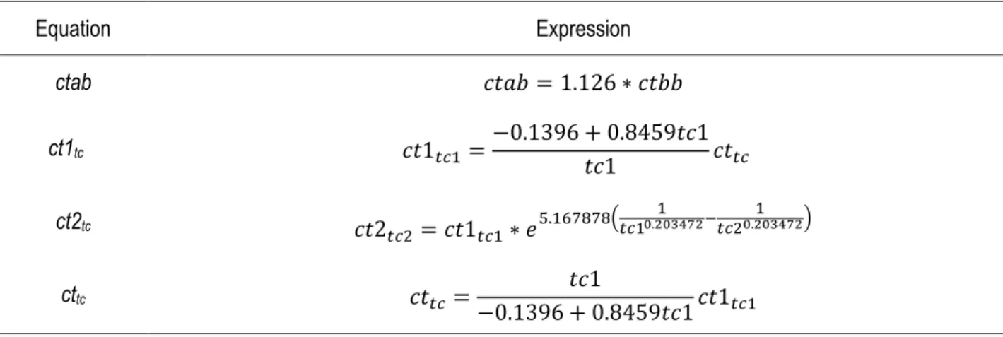
The model for predicting cork biomass at 9 years of age is dependent from cork thickness after boiling at 9 years of age too. For that reason, the cork thickness after boiling at 9 years of age had to be found. In Almeida and Tomé (2008) a system of equations that allows the prediction of mature cork caliber over time can be used in this purpose. Some of them have been used in the present work (see Table 3): (I) a model to transform cork thickness before boiling to cork thickness after boiling; (II) a model to find growth of complete rings (years) at t years depending on the thickness of complete rings at any other age; (III) a model that founds the caliber after boiling as a function of the thickness of complete years; and (IV) a model to transform the same as before but in the other sense.
Table 3: System of equations from Almeida and Tomé (2008) used for the estimation of the 9 years cork thickness value after boiling, used as an independent variable in Paulo and Tomé (2010) model IV.
Equation Expression ctab 𝑐𝑡𝑎𝑏 = 1.126 ∗ 𝑐𝑡𝑏𝑏 ct1tc 𝑐𝑡1𝑡𝑐1=−0.1396 + 0.8459𝑡𝑐1 𝑡𝑐1 𝑐𝑡𝑡𝑐 ct2tc 𝑐𝑡2 𝑡𝑐2= 𝑐𝑡1𝑡𝑐1∗ 𝑒 5.167878( 1 𝑡𝑐10.203472− 1 𝑡𝑐20.203472) cttc 𝑐𝑡𝑡𝑐= 𝑡𝑐1 −0.1396 + 0.8459𝑡𝑐1𝑐𝑡1𝑡𝑐1
ctab, cork thickness after boiling (mm); ctbb, cork thickness before boiling (mm); ct1i, cork thickness of the first complete i rings (mm); tc1,
number of complete rings (years); ct1tc1, cork thickness in tc1 complete years (mm)
The procedure that has been followed to get cork thickness after boiling at 9 years of age is synthetized in Figure 5.
Figure 5: Procedure by steps of the transformations by equations of the data, from cork caliber at t years to cork caliber at 9 years of age.
Caliber at t years before boiling (ctbbt) • ctbb13 • ctbb8 Caliber at t years after boiling (ctabt) • ctab13 • ctab8 Caliber for t-1 complete growth years • ct112 • ct17 Caliber for 8 complete years • ct18 • ct18 Caliber at 9 years • ctab9 • ctab9
3. Methods
14 3.2. Predicting cork bark weight proportion at 9 years of age (cbp9)
Paulo and Tomé (2010) showed that the cork back proportion (cbp9) presented significant relationship to cork thickness after boiling, and used this variable (ctab) to develop the following model:
𝑐𝑏𝑝 = 𝑒𝑥𝑝 [− [ 𝑐𝑡𝑎𝑏𝑡 (19.4629)]
0.4744
]
Once the cork caliber at 9 years of age has been found (section 3.1), the cork bark proportion at 9 years of age (cbp9) can be derived directly from this model.
3.3. Validation of the Paulo and Tomé (2010) method
The objective of the validation was to analyse and characterize the errors of the models that were used to find out the mature cork biomass for corks of different ages when used jointly with the model of cork back percentage (Paulo and Tomé, 2010) and the system of equations of Almeida and Tomé (2008) to predict cork caliber at 9 years from calibre measured at any other cork age
Validation of the models is a very important step in model evaluation because quality of fit does not necessarily reflect the quality of prediction. Any model is a simplification of the reality and cannot be correct in every sense. Models used in decision support require a firm foundation in science and should produce predictions with qualified accuracy (Burkhart and Tomé, 2012). Validation involves a process to determine if a model performs at an acceptable level for its intended purpose (Burkhart and Tomé, 2012). Validation is the act of increasing to an acceptable level the confidence that an inference about a simulated process is correct for the actual process (Van Horn, 1971). Model validation can never result in the acceptance of a model as right or wrong. It is instead a thorough analysis of model performance, including several procedures, that provides information that can be used to assess its adequacy for a particular use (Burkhart and Tomé, 2012).
Yang et al. (2004) recommended that analysts look at how well a model fits new, independent data rather than apply a statistical test to determine whether or not the model is good enough, because results will vary depending on the data, model types, study objectives, and statistical test applied. Model validation is an attempt to judge whether or not a model is an acceptable representation of the reality for some stated purpose. The model evaluation in this case is focused on the validation, a quantitative analysis that implies comparisons of predictions with observations
3. Methods
15 independent from those used to fit the model, usually including statistical evaluation of the magnitude of the differences between the model and the real world (Burkhart and Tomé, 2012).
The analysis of the logic behind the model structure, including the model components, and of the compatibility of the model predictions with existing biological theories are usually referred to as qualitative evaluation. The model must be biologically realistic, agree with existing theories of forest growth and predict sensible responses to management actions (Burkhart and Tomé, 2012).
Analysis of model error is based on the computation of prediction residuals or model errors, the differences between the observed and predicted values of all variables of interest. Error characterization may involve statistical testing or be based mainly on the computation of selected statistics and graphical analysis (Burkhart and Tomé, 2012).
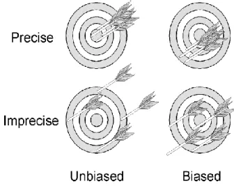
Model error should be assessed in terms of two characteristics: bias and precision (Figure 6). Bias refers to the deviation of the average of the model errors from zero and the precision to the size of the model errors.
Figure 6: Schematic representation of bias and precision terms (Vanclay, 1994).
The most commonly used statistics to assess bias and precision are the mean value of the residuals (Mr) for the bias and mean of the absolute value of the residuals (MIrI) to evaluate precision:
3. Methods 16 Model bias: 𝑀𝑟= ∑𝑛𝑖=1(𝑦𝑖− 𝑦̂𝑖) 𝑛 Model precision: 𝑀|𝑟| = ∑𝑛𝑖=1|𝑦𝑖− 𝑦̂𝑖| 𝑛
Where yi is the observed cork weight of tree i, 𝑦̂𝑖 is the estimated value of cork weight of tree i using the Paulo and
Tomé (2010) method and n is the number of observations used in the validation procedure.
The analysis of the distribution of the errors may also be useful to assess precision. The 5% and 95% percentiles are commonly calculated statistics as they are not overly sensitive to extreme points in the data. Plots of observed versus predicted values are another way to characterize bias and precision.
Another statistic frequently used to compare predictions is the so-called modelling efficiency:
𝑒𝑓 = 1 −∑(𝑦𝑖− 𝑦̂)𝑖
2
∑(𝑦𝑖− 𝑦̅)𝑖 2
where yi is the observed cork weight of tree i, 𝑦̂𝑖 is the estimated value of cork weight of tree i and 𝑦̅ is the cork 𝑖 weight average value.
Model efficiency (ef) provides a simple index of performance on a relative scale, where 1 indicates a “perfect” fit, 0 reveals that the model is no better than a simple average, and negative values indicate a poor model indeed (Burkhart and Tomé, 2012).
Since the final objective was to develop a method that is able to predict cork biomass for corks with different ages, the validation statistics were also computed separately according to cork age. Validation was also carried out for each model separately (model I, II, III and IV), by diameter classes (5 cm range), cork thickness classes and the number of first-order debarked branches.
Since the cork biomass increases with tree size, namely with diameter, it was expected to find larger values of the residuals in larger trees. Nevertheless, these larger values of residuals do not necessarily correspond to lower precision of the model, since they may represent a small percentage of the total cork biomass produced by a tree with
3. Methods
17 large dimensions. Therefore, when evaluating bias, the mean of the absolute value of the residuals was also computed in percentage as suggested by Paulo and Tomé (2010):
𝑀|𝑟
𝑗|= 100
∑𝑛𝑖=1|(𝑦𝑖− 𝑦̂ )|𝑖 /𝑛𝑗
𝑐𝑗
where yi is the observed cork weight of tree i, 𝑦̂𝑖 is the estimated value of cork weight of tree i, nj is the number of observations in class j, and cj is the mean value of cork biomass from class j.
4. Results
18
4.
RESULTS
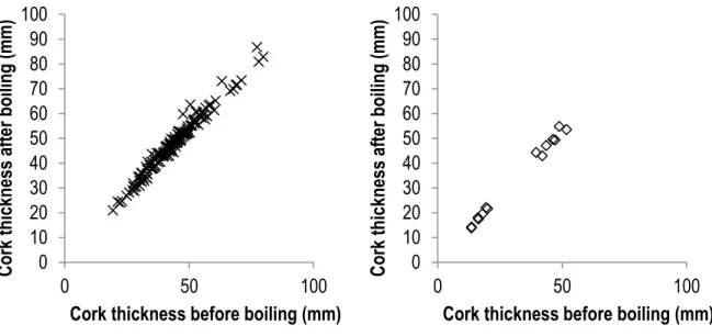
Cork boiling of the samples resulted in an increase of cork thickness (Figure 7) varying between 1.18 and 25.99%, with an average value of 9.17%.
Figure 7: Relationship between cork thickness after and before boiling in mm: x, cork with 13 years (left) and ◊, with 8 years (right).
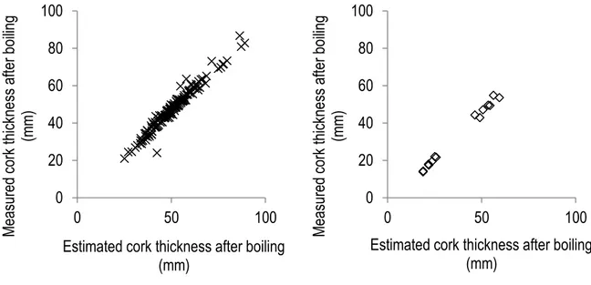
The estimation of cork biomass predicted with model IV required the estimations of cork thickness values for 9 years of age (ctab9), included as a variable in model IV, was made twice
i) using the measured values of cork thickness showed in Figure 7 (ctab_m);
ii) using the Almeida and Tomé (2008) systems of equations presented in Table 3 (ctab_e).
Both of them were transformed into ctab9_m and ctab9_e following the same procedure described in section 3. Differences in the estimated values from both alternatives are presented in Figure 8. In absolute values, they vary between 0.01 mm and 18.36 mm, with an average value of 3.51 mm difference (ctab_m - ctab_e). The validation has been done using both alternative values in model IV (ctab9_m and ctab9_e), demonstrating that no important differences were encountered (not shown). For this reason, only the results obtained considering the ctab_m were presented.
0
10
20
30
40
50
60
70
80
90
100
0
50
100
Co
rk
thic
knes
s
aft
er
boili
ng (
mm)
Cork thickness before boiling (mm)
0
10
20
30
40
50
60
70
80
90
100
0
50
100
Co
rk
thic
knes
s
aft
er
boili
ng (
mm)
4. Results
19
Figure 8: Relationship between cork thicknesses after boiling measured directly and estimated by Almeida and Tomé (2008) system of equations in mm: x, cork with 13 years (left) and ◊, with 8 years (right).
The validation statistics, considering as a validation data set the samples collected for this thesis (8 and 13 years old cork) plus the ones used by Paulo and Tomé (2010) (9, 10 and 11 years old cork), showed an increase of model efficiency and a general reduction of residuals and absolute residuals when moving from model I to model IV as alternative models for the estimation of cork biomass with 9 years old. Indeed, the Paulo and Tomé (2010) method performs better when model IV was used instead of model III, and this was even more evident when comparing validation estimates resulting from models I and II (Table 4).
Table 4: Validation statistics obtained from the Paulo and Tomé (2010) method, considering together as a validation data set the samples collected for this thesis (8 and 13 years old cork) and the ones used by Paulo and Tomé (2010) (9, 10 and 11 years old cork). Statistics are presented separately considering the usage of alternative models I, II, III and IV for the estimation of cork biomass with 9 years old (see section
3 for details). Model Mr MIrI P5 P95 ef I 2.86 11.62 -0.49 40.32 0.71 II 3.06 10.87 -0.38 38.84 0.71 III 2.91 7.80 0.12 25.42 0.85 IV 2.23 6.38 0.23 19.60 0.90
Mr, mean value of the residuals (kg); MIrI, mean of absolute value of the residuals (kg); P5, percentile 5 of the
residuals (kg); P95, percentile 95 of residuals (kg); ef, model efficiency
0
20
40
60
80
100
0
50
100
M
ea
su
red
co
rk th
ickne
ss
aft
er
bo
iling
(mm)
Estimated cork thickness after boiling
(mm)
0
20
40
60
80
100
0
50
100
M
ea
su
red
co
rk th
ickne
ss
aft
er
bo
iling
(mm)
Estimated cork thickness after boiling
(mm)
4. Results
20 4.1. Results according to cork age
For detailing the validation procedure according to cork age, the number of observations available by cork age was computed (Table 5).
Table 5: Frequency distribution for cork age (years).
Age (years) Frequency
8 14
9 100
10 90
11 93
13 146
Models I and II showed lower and similar values of model efficiency for all cork ages (Figure 9). Similar model efficiency values were also found for models III and IV, for these varying between 85% and 95%. In relation to cork age, models I and II perform better for 9 and 10 years old cork, while models III and IV were the ones that showed a smaller variation of model efficiency across different cork ages, although, in general, all models presented a decrease of model efficiency for cork ages of 11 and 13 years.
Figure 9: Model efficiency along 8, 9, 10, 11 and 13 years of cork ages for the different models tested.
0,0 0,1 0,2 0,3 0,4 0,5 0,6 0,7 0,8 0,9 1,0 7 8 9 10 11 12 13 14 Model efficiency
Cork age (years)
4. Results
21 Mean value of residuals for bias assessment again showed similarity between the values obtained by the four models, in the case of cork ages between 9 and 13 (Figure 10). Instead, for cork age equal to 8 years, models III and IV clearly outperformed models I and II. For facilitating the observation of the tendency of the values, the mean value of the residuals was shown separately for models III and IV (Figure 11).
Figure 10: Bias of the tested models with cork age – mean value of the residuals (kg).
Figure 11: Bias of model III and IV with cork age – mean value of the residuals (kg).
-25 -20 -15 -10 -5 0 5 10 15 7 8 9 10 11 12 13 14 Mean value of t he r esiduals (kg)
Cork age (years)
Model I Model II Model III Model IV
-4 -2 0 2 4 6 8 10 7 8 9 10 11 12 13 14 Mean value of t he r esiduals (kg)
Cork age (years)
4. Results
22 When the mean value of the residuals was computed in percentage (Figure 12) the shape of the curves was similar, now showing an increase for positive bias estimates in all the models when cork age goes from 11 to 13. Bias was larger in models I and II for 8 years, reaching values of -19 and -22 kg (-23 and -26% in percentage). The bias was smaller in 9, 10 and 11 years, and for 13 years both models showed a bias that varied from 6.69 to 9.17 kg. For younger ages (8 years) models I and II overestimated cork biomass and, in the opposite way for older cork ages (13 years) all the models (models I to IV) underestimate the cork biomass.
Figure 12: Bias of the tested models with cork age – mean of value of the residuals (%).
Analysing the precision using the mean value of the absolute residuals in percentage of cork biomass (Figure 13) showed that again models I and II were generally less precise (values ranging between 23 and 46%), and that more evident differences were found for 8 and 13 years old cork. For corks with 9, 10 or 11 years old, precision was similar for models I and II and for models III and IV. The biggest percentages in absolute values were found in models I and II for 8 and 13 years, reaching values of 46.39 and 37.19%, respectively. The more the complexity of the model the more precise the cork biomass estimates were. Precision of model III varies for all ages from 15.60 to 27.61% and for model IV from 13.01 to 22.03%. The tendency for models III and IV seems to be better as more close to age 10 and worst in the extremes, 8 and 13 years.
-30 -20 -10 0 10 20 30 7 8 9 10 11 12 13 14 Mean value of t he r esiduals (%)
Cork age (years)
4. Results
23
Figure 13: Precision of the tested models with cork age – mean of absolute value of the residuals (%).
4.2. Results according to diameter under cork
The next step, in order to find out if the results obtained for bias and precision were related with cork age or with other tree variables, was carried out by checking the performance of the models independently of the age and centred on other variables that may be also sources of error. First a possible relationship between error values and the distribution of the tree diameter classes was observed. Frequency of the distribution is shown in Table 6. All classes have at least 20 cork samples except class 60 cm that only has 10 cork samples.
0 5 10 15 20 25 30 35 40 45 50 7 8 9 10 11 12 13 14 Mean of absolu te value of t he residuals (%)
Cork age (years)
4. Results
24
Table 6: Frequency distribution for diameter under cork classes (cm).
Diameter under cork
class (cm) Frequency 20 39 25 82 30 83 35 65 40 60 45 35 50 25 55 21 60 10 > 65 23
Model efficiency (Figure 14) across all diameter classes varied less for models III and IV, with minimum values of 0.61 and 0.73 for diameter classes 45 and 40 cm, respectively. Instead, for models I and II, model efficiency markedly decreased for diameter classes between 40 to 50 cm reaching values of 0.12 and 0.27.
Figure 14: Model efficiency for diameter under cork classes (cm) for the different tested models.
0,0 0,1 0,2 0,3 0,4 0,5 0,6 0,7 0,8 0,9 1,0 0 5 10 15 20 25 30 35 40 45 50 55 60 65 70 Model efficiency
Diameter under cork class (cm)
4. Results
25 Figure 15 represents the mean value of the residuals (kg) along diameter classes. All the models were positively biased but less in the diameter classes below 45 cm and the cork class 60 cm (that only has 10 cork samples), and model IV was less biased than the others. In a medium diameter class under cork, as an example class 55 cm, it was possible to find bias values that vary from 12.33 kg in model IV to 17.94 kg in model I (represent values of 15 and 22% in percentage, respectively; see Figure 16). If the class 60 cm was ignored, because of the few data inside that class, it was possible to see a tendency on the bias increasing from the class 40 cm forward.
According to Figure 17 the same values commented before were represented in absolute values as 21 and 34% in absolute values for models IV and I, respectively. Clearly model I was the less precise and model IV the more precise. The tendency of precision was that as the diameter under cork increases the percentage of the absolute residuals also increases in models I and II, but for models III and IV the average tendency is flat.
Figure 15: Bias of the tested models with diameter under the cork – mean value of the residuals (kg).
-5 0 5 10 15 20 25 0 5 10 15 20 25 30 35 40 45 50 55 60 65 70 Mean value of t he r esiduals (kg)
Diameter under cork class (cm)
4. Results
26
Figure 16: Bias of the tested models with diameter under the cork – mean of value of the residuals (%).
Figure 17: Precision of the tested models with diameter under the cork – mean of absolute value of the residuals (%).
-10 -5 0 5 10 15 20 25 0 5 10 15 20 25 30 35 40 45 50 55 60 65 70 Mean value of t he r esiduals (%)
Diameter under cork class (cm)
Model I Model II Model III Model IV
0 5 10 15 20 25 30 35 40 0 5 10 15 20 25 30 35 40 45 50 55 60 65 70 Mean of absolu te value of t he residuals (%)
Diameter under cork class (cm)
4. Results
27 4.3. Results according to cork thickness classes
Similar plots for industrial cork thickness classes (Figure 18 to Figure 21) showed that all the models follow the same tendency of bias overestimating cork biomass of thinner cork classes and underestimating cork biomass for thicker classes but always the less biased was the model IV. According to precision, models I and II were clearly less precise and model IV was more precise than model III. All models respond better in bias and precision in thin, half stand,
standard and large cork thickness classes. In this particular case the tendency of model IV was quite different and
also much better than the other models. In relation to other variables, models III and IV behaved similar but in what concerns the relationship between the errors and cork thickness the position of model IV was indisputably better. The distribution of the frequencies and the intervals of the classes are shown in Table 7. All cork thickness classes had at least 40 samples.
Table 7: Frequency distribution and intervals (in mm) for cork thickness classes.
Cork thickness class Cork thickness interval (mm) Frequency
Extra thin <22 50 Thin 22-27 66 Half stand 27-32 77 Standard 32-40 78 Large 40-54 129 Extra large >54 43
Model efficiency (Figure 18) shows that all models were above 0.5, and skipping the extreme classes, extra thin and
extra large, all models had efficiency above 0.7. The response of models IV and III was really close to 1 and more or
4. Results
28
Figure 18: Model efficiency for cork thickness classes for the different tested models.
Figure 19: Bias of the tested models with cork thicknesses classes – mean value of the residuals (kg).
0,0 0,1 0,2 0,3 0,4 0,5 0,6 0,7 0,8 0,9 1,0 Model effiency Cork thickness
Model I Model II Model III Model IV
-15 -10 -5 0 5 10 15 20 25 30 35 Mean value of t he r esiduals (kg) Cork thickness
4. Results
29
Figure 20: Bias of the tested models with cork thicknesses classes – mean value of the residuals (%).
Figure 21: Precision of the tested models with cork thickness classes – mean of absolute value of the residuals (%).
-40 -30 -20 -10 0 10 20 30 40 50 Mean value of t he r esiduals (%) Cork thickness
Model I Model II Model III Model IV
0 5 10 15 20 25 30 35 40 45 Mean of absolu te value of t he residuals (%) Cork thickness
4. Results
30 4.4. Results according to the number of first-order debarked branches
Finally, the same analysis was performed according to the variable number of first-order debarked branches. It is important to clarify that for this variable, a value equal to 1 corresponds to a tree that was only debarked in the stem. When this variable takes a value equal or larger than 2, it corresponds to the number of first-order branches debarked. The frequency of distributions for the validation data set observations (Table 8) showed that most of the trees had only been debarked in the stem, and that a few ones have been debarked in 4 or more first-order branches (12 observations).
Table 8: Frequency distribution depending on number of first-order debarked branches.
Number of debarked branches Frequency 1 268 2 120 3 43 4 9 5 3
Model efficiency (Figure 22) across the number of debarked branches varied from 0.57 to 0.98. Tendency of models III and IV was constant independently of the branches debarked, but in models I and II there was a peak at 4 debarked branches; deteriorating the performance of the models as more debarked branches were added in the debarking operation, but recovering at 5.
4. Results
31
Figure 22: Model efficiency for number of debarked branches for the different tested models.
The peak in bias was at 5 first-order debarked branches (Figure 23) that reaches 28 kg (24% in percentage; see Figure 24) of biomass in model I; but focusing on precision (Figure 25), at the same point, is when all models were more precise, telling us that the biomass that the models estimate when 5 branches are debarked do not represent so much in proportion of tree cork biomass, that was very large in these big trees. Precision of all models was worst when 4 branches are debarked.
If trees with 5 debarked branches were not considered, bias decreases varying from values around 10 to -5 kg (19 and -12% in percentage of residual values, respectively) of cork biomass that represent values around 16 till 40% in precision.
Following the previous results it was also evident here that models I and II perform worse than models III and IV, and model IV was the less biased and the more precise.
0,0 0,1 0,2 0,3 0,4 0,5 0,6 0,7 0,8 0,9 1,0 0 1 2 3 4 5 6 Model efficiency
Number of debarked branches
4. Results
32
Figure 23: Bias of the tested models with number of debarked branches – mean value of the residuals (kg).
Figure 24: Bias of the tested models with number of debarked branches – mean value of the residuals (%).
-10 -5 0 5 10 15 20 25 30 0 1 2 3 4 5 6 Mean value of t he r esiduals (kg)
Number of debarked branches
Model I Model II Model III Model IV
-15 -10 -5 0 5 10 15 20 25 30 0 1 2 3 4 5 6 Mean value of t he r esiduals (%)
Number of debarked branches
4. Results
33
Figure 25: Precision of the tested models with number of debarked branches – mean of absolute value of the residuals (%).
0 5 10 15 20 25 30 35 40 45 0 1 2 3 4 5 6 Mean of absolu te value of t he residuals (%)
Number of debarked branches
4. Results
34 4.5. General results
Comparing model efficiency along cork ages, it was found that for all models it was above 0.5, but that models III and IV outperformed models I and II for all cork ages. Since for corks with 8 years models I and II showed to be biased, their response in terms of precision have a poor performance in ages 8 and 13 years. The bias and precision of models III and IV seem quite well for all cork ages.
The analysis of the relationship between model errors and tree diameter under cork classes showed that all of them performed poorly for some diameter classes, with an increasing error tendency for higher tree diameter values. When looking in detail for the characteristics of the sample by diameter classes, it can be noted that the pattern of average cork thickness by diameter class follows a pattern somehow similar to the one observed for the errors in cork biomass prediction (Figure 26). In terms of bias all models followed the same trend, being more imprecise as the diameter of trees increase. Instead, for models III and IV, the tendency of the precision was less noticed.
Figure 26: Relationship of average value for 8 complete years cork thickness (mm) and by 5 cm range tree diameter under cork classes (cm).
Focusing the analysis of the residuals computed by cork thickness classes, it was found that considering the caliber, variable improves the mean value of the residuals more than 20% for the extra thin class and 10% for the extra large class in comparison to model III. This again noticed the importance of the cork thickness variability between trees, even with the same diameter, debarked height and number of debarked branches. For average values of cork
22 24 26 28 30 32 34 0 5 10 15 20 25 30 35 40 45 50 55 60 65 70 C or k thickness of 8 complete years (mm)
4. Results
35 thickness the differences between the models were more or less following similar to the trend observed in the analysis with other variables, that model I and II were worse than models III and IV. But for the extreme values, only model IV could be considered appropriate in terms of bias and precision. Model IV was the one less biased for all cork thickness classes. The tendency of bias was similar in all models for all cork thickness classes overestimating cork biomass for thinner classes and underestimating cork biomass for large classes but the performance of model IV was always better. These results suggest the need to improve the existing models to predict cork biomass in order to decrease the bias that was observed for values of cork thickness that were outside the more usual range of cork thicknesses.
Finally the analysis with number of first-order debarked branches showed a good performance of the efficiency for all models being better models III and IV in comparison to models I and II but all above 0.5. When the attention was focused on trees with 5 first-order debarked branches it was found that all models were biased, more than when the number of debarked branches was lower, but this bias also represents the best precision in percentage, telling us that the proportion of error in the prediction of biomass for those trees was not so high. On the other hand, the focus was on the lower number of debarked branches and when that number was 4 the precision reached around 40% (model I) of the mean value of the absolute residuals but almost 24% in model III.