Valter Vairinhos1, Rui Parreira2, Suzana Lampreia3, Vítor Lobo4, and Purificación Galindo5 1 Cinav, Escola Naval, Portugal and ICAA, Santarém, Portugal
valter.vairinhos@sapo,pt 2,3 Cinav, Escola Naval, Portugal
[email protected] [email protected]
4 Cinav, Escola Naval, Portugal and ISEGI, UN, Portugal [email protected]
5 Depto. de Estadística Universidad de Salamanca, España [email protected]
ABSTRACT
Vibration Analysis (VA) is now routinely used for condition monitoring and failure diagnosis in Condition Based Maintenance (CBM). In the context of VA, a methodology is proposed, based on biplots, to simultaneously display both vibration frequencies and their measurement points, in support of monitoring and diagnostics tasks.
In this research, real observational data obtained measuring mechanical vibrations on four generators aboard a Portuguese Navy Ship in real operating conditions is used. A portable vibration collector was employed, and the measurements were taken at 13 measurement points in each one of four generators, using the same collector settings. Spectrograms resulting from vibration measurements were transformed into biplots and used for decision support according to the proposed methodology. Data analysis showed a robust stability in the macrostructure of biplots when observations resulting from different generators of the same model and at the same assumed conditions was analyzed. This invariance allows the specification of reference conditions, rules to detect changes of operating conditions and the emergence of failures. The proposed methodology, once embedded in dedicated software, will reduce the interpretation error in diagnosis and prognosis associated to variability in personnel training and experience. Consequently, it will increase the safe use of VA in an increasing number of situations.
1. INTRODUCTION
VA is nowadays an efficient, reliable and proven methodology, widely used for CBM.
This being true, its use in some organizations poses problems connected not with the method itself but with its organizational implementation. One important issue that limits its generalized use in some contexts is related with personnel training and retention.
The routine use of VA implies investments in equipment and personnel training. Performing accurate measurements and correct interpretations of data analysis results are not trivial tasks. Only technicians with solid theoretical knowledge about the methodology and accumulated practical experience can reliably perform these tasks. This means that those technicians become highly valuable for the organization which employs them and, at the same time, become very attractive for other organizations.
For government and other organizations lacking competitive salaries and having high internal mobility, it becomes very difficult to retain that kind of personnel: Therefore, very frequently, the introduction of VA based CBM becomes, in practice, a never-ending process and, sometimes, a practical impossibility. To overcome this situation, a partial solution is to incorporate a greater part of the knowledge involved in software.
Recent emergence of low cost sensors, frequently enabling wireless data transmission, local data storage and processing also lead to a need for better software tools. The amount of data collected both by sensors and mobile data collectors is becoming bigger every day and the problem associated with
_____________________
Valter Vairinhos et al. This is an open-access article distributed under the terms of the Creative Commons Attribution 3.0 United States License, which permits unrestricted use, distribution, and reproduction in any medium, provided the original author and source are credited.
its storage, handling and analysis is one of the present challenges to statistics and computation, as discussed by Ferrer (2014). In this context, the present paper proposes the use of biplots as a graphical and descriptive instrument to consider in the development of software for VA.
Field data associated to VA has an observational nature: data used for analysis in an operational setting is frequently collected using portable collectors, operated by not always fully trained technicians, in aggressive environments (heat, noise, smell, movement, reduced space) very far away from controlled laboratory conditions where planned experiments make sense. For this kind of data, sophisticated statistical inference procedures are in general invalid, given failure to satisfy assumed theoretical conditions such as randomness and independence.
With the strong emergence of low cost sensors and the development of “Internet of Things” (IoT) all this is changing. The data generated daily from thousands of such sensors installed in a single plant (a ship for instance) allows not only the use of sophisticated multivariate data analysis methods but also imposes the search for new data driven methodologies able to cope, in real time, with such “data mountains”.
The structure of this work is as follows. Part 2 is devoted to the statistical formulation of VA based CBM. Here it is shown that equipment condition is a latent, not directly observable variable, that manifests itself through observations at a chosen set of Observation Points (OP), and that must be estimated and predicted using adequate statistical methodologies. Part 3 is a brief review of relevant methodological literature directly related with our problem. Part 4 presents materials and methods employed, including collected data and assumptions implicit in its analysis. Part 5 is used to define a kind of biplots assumed useful for the interpretation of VA data, relating OP with Fourier Frequencies (FF). Part 6 is used to interpret relations that can be read from biplots built from spectrograms and to present rules to detect, characterize and forecast failures using biplots.
2. VIBRATION ANALYSIS AND CBM
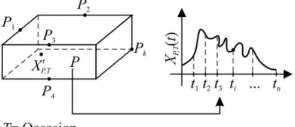
In VA CBM it is assumed that the machine condition (in general not directly observable) manifests itself through the vibration signals measured at a pre-defined set of observation points (OP) on the machine. See Figure 1, where the machine is represented as a parallelepiped and the selected observation points set is represented by OP = { P1, P2, … , Pk, …, PK }. This means that it is assumed that the
true condition of the machine (whatever its meaning) manifests itself through the vibration signals observed at OP. Frequently, the set OP is suggested by equipment builder or imposed by local physical practical conditions such as accessibility, temperature or other. This means that neither the number of points nor its locations are necessarily
Figure 1. For a specific equipment, the points P1, P2, … , Pk, …, PK represent observation points where the vibration
energy is represented by XP, tT( ), t= 1, …, n at the specific occasion T.
optimal from the point of view of condition estimation, this fact making room for further theoretical considerations Let
XP,T(t),t0,T =1,2,...,Q
(1)represent the vibration signal, expressed in a convenient measurement unit (in fact it could be displacement, velocity, or acceleration) at a specific point P and observation occasion T= 1, 2, …, Q. XP,T (t) is a stochastic process, i.e. a
random variable dependent of time. The sequence of observation occasions T= 1, 2, …, Q must not be confused with time t used to refer to the time parameter of a specific signal. For example, P may represent the left support of a specific Diesel engine, T refer to weekly observations of that engine and t (in seconds) a generic instant in the interval [0, 1], 1 second being the observation length. Expression (1) is a continuous stochastic process that must be observed at specific instants (t1, t2, …, ti, …, tn) specified
by n (sampling rate).
This means that the observed data for a specific measurement occasion (T) is a set of K observed time series, each one with n observations as can be seen in Table 1. The “true” machine condition at a specific occasion is not directly observable and must be estimated, predicted or inferred from the observed time series data at OP for a succession of occasions (observation times).
) ( , 1 t XP T → , (1)... , ( )... , ( ) 1 1 1T PT i PT n P t X t X t X … … ) ( , t XPT → XP,T(t1)...XP,T(ti)...XP,T(tn) … … ) ( , t XP T k → XPk,T(t1)...XPk,T(ti)...XPk,T(tn)
P -Observation Point; T= Observation Occasion Table 1. Observed time series corresponding to K observation points, at occasion T. For each point, the
Referring to one such specific time series as x1, x2, …, xn,
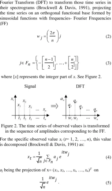
the usual VA procedure consists in using the Discrete Fourier Transform (DFT) to transform those time series in their spectrograms (Brockwell & Davis, 1991), projecting the time series on an orthogonal functional base formed by sinusoidal functions with frequencies- Fourier Frequencies (FF) j n j w
= 2 (2)
− + − = 2 , ... , 2 1 n n n F j (3)where [x] represents the integer part of x. See Figure 2.
Figure 2. The time series of observed values is transformed in the sequence of amplitudes corresponding to the FF. For the specific observed value xt (t= 1, 2, …, n), this value
is decomposed (Brockwell & Davis, 1991) as: = n F j j itw e j a n t x 1 (4)
aj being the projection of x= (x1, x2, …, xi, …, xn)T on
j itw e n 1 . (5)
Inference about machine condition is then performed using statistical inference procedures based on results of DFT, or, informally, using the analyst skills, knowledge, experience and on existing rules or regulations.
3. LITERATURE REVIEW
The inference problem associated with spectral analysis and, consequently, with the use of VA for CBM, is solved using the concept of spectral density function and its estimation through the periodogram, a function of FF (w) and observed signal values xt (t= 1, …, n). If f(w) is the theoretical
spectral density function, the variance or energy contained in the signal for frequencies w is given by
dw w f w w dF w
w
F( )= − ( )= − ( ) . (6) distribution (Priestley, 1981, and Brockwell & Davis, 1991).
Statistical inference about f(w) is based on the observed data periodogram and its sampling distribution (Brockwell & Davis, 1991). This problem has been the object of intense research during the last 50 years, as can be seen in Jones (1965), Beneke, Leemis, Schelegal and Foote (1988), McSweeney (2006) and, more recently, in Fokianos and Savvides (2008). In all those references the main issue is to decide if two periodograms, corresponding to two sets of observations, come from the same population spectral density or not. For recent work in this direction see also Halliday, Rosenberg, Rigas and Conway (2009), and Ravishanker, Hosking and Mukhopadhyay (2010).
Unfortunately, the use of these statistical inference results for operational diagnostic needs is questionable given the observational nature of data collected, not satisfying all the theoretical assumptions required by inference methods. In consequence, the diagnostic decision based on results of DFT is in general performed informally by the technicians, using their knowledge, experience and judgement.
This context is changing with the availability of low cost high quality sensors. This creates a super abundance of data allowing and imposing the use of multivariate data analysis methods (Garcia & Trendafilova, 2014, Ferrer, 2014), where a new paradigm for Statistical Process Control (SPC) is identified and the generalized use of multivariate data analysis methods is suggested. Frequently these methods are based on the decomposition of matrices and other tensors using the Singular Value Decomposition (SVD) and in the visualization of its results. That is the case for classical multivariate techniques such as principal components (Li, Shi, Liao & Yang, 2003).
The use of multivariate data analysis techniques in the context of maintenance has been the object of many contributions such as Zhan, Makis and Jardine (2003). The use of biplots in maintenance, proposed in this paper, has scarcely been employed. The biplot concept and its variants can be seen in Gabriel (1971), Galindo (1986), Greenacre (2010), Gower and Hand (1996).
Biplots were initially proposed by Gabriel (1971). The concept was also present in the work of French school of Benzécri, associated to correspondence analysis (Benzécri et Collaborateurs, 1973). Biplots show in the same plot two kinds of objects (two modes), for example, frequencies and observation points. As can be seen in what follows, VA and reasoning involved in interpretation and prognosis relates more than two kinds of objects; namely: Occasions, Observation Points, Frequencies and Equipment.
For this multiway or multimode data, occurring naturally in VA, a whole set of statistical and visualization methodologies have been developed recently (Kroonenberg, 2008, Papalexakis & Faloutsos, 2015, Kolda & Sun, 2008, Mendes, 2011, Mendes, Fernandez-Gomez, Pereira, Azeiteiro & Galindo-Villardon, 2012). It is expected that, in
the near future, more applications of these concepts to VA and CBM will show up.
4. MATERIAL AND METHODS.DATA ISSUES
Data for this work was collected by the second author in real operating conditions on board NRP Berrio, a Portuguese Navy auxiliary ship. The data was obtained measuring vibration signals (in g-s) from four electrical power generators, powered by Volvo Penta TAMD 165A Diesel engines. These are four strokes, direct injected, turbocharged 440 kw, 1800 rpm diesel engines. The AC generators are STAMFORD, HC M534 D1, 60Hz, 487.5 kw at 1800 rpm.
For each one of the 4 Generators (GE1 to GE4), vibrating signals were measured at K= 13 OP, identified in Figure 3, using a mobile collector CSI 2140 from Emerson (Emerson, 2016).
The vibration collector CSI 2140 was set for Hamming Window, observation time 1 second and sampling rate 3900 lines. For each measurement, several replicas were obtained (at least 3) and the corresponding DFT’s were averaged. Figure 4 shows one possible layout for DFT resulting data. For each equipment E (power generators GE1 to GE4), at a specific point P, and a spectral frequency w, the corresponding amplitude (g-s) was aE,P,w.
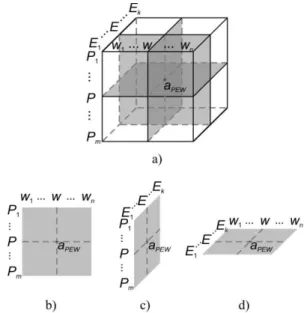
This kind of data is a 3-way layout (three modes) since it relates 3 kinds of entities: Equipment, Points and Frequencies. If all the measurements were obtained at the same occasion (T= 1st February 2011) for the 4 groups, the 3-way layout that interests us here is shown in Figure 4 a). This kind of data, represented by tensors of order ≥ 2, requires algorithms such as PARAFAC (Kroonenberg, 2008, Papalexakis & Faloutsos, 2015, Kolda & Sun, 2008, Mendes, 2011) to generalize to higher dimensions the classical graphical results such as principal components and biplots based SVD.
2D Biplots used in this work were drawn using the software Biplots PMD (Vairinhos, 2003).
Figure 3. For each site (1, 2, ...,7) there are 1, 2 or 3 measurement points labelled as P(A,H,V). For example, P4
(A, H, V) means that at site Coupling (C) there are 3 measurements points – Axial, Horizontal and Vertical.
Figure 4. a) A 3-way layout with modes 1 – Observation Points (P); 2 –Frequencies (w); 3 – Observed Equipment (E); b) Slices corresponding to biplots of interest. For Point
p (on each equipment), relation between frequencies and equipment; c) For w0= 30HZ, say, aEPw – amplitude for E, P,
w constant, relation between Equipment and OP. The suggested use of biplots in what follows is based in the following two assumptions:
Assumption 1- The equipment condition does not change during the measurement process, at a specific occasion, for different OP.
Assumption 2- The vibration patterns observed at OP (expressed by the corresponding DFT´s) are related. This relation is assumed approximately linear and captured by DFT’s correlations.
5. USING BIPLOTS TO STUDY SPECTROGRAMS
Biplots are defined in Gabriel (1971) as follows: given a rectangular matrix X (np) with n rows and p= m columns, this matrix can be represented exactly in Rr, with r= rank
(X) p, or, approximately, in Rd with d < rank (X), using a
Cartesian reference system, representing its rows by markers g1 … gn and markers h1 … hr for the columns, this
representation being called a biplot, with x =ij giThj (i= 1 … n; j= 1 … p).
Given the SVD of X = UΣVT = UΣαΣ(1-α)VT , ( 0 <= α <= 1) where U and V contain X´s left and right eigenvectors and diagonal matrix Σ contains its singular values, one possible choice for markers, satisfying Gabriel definition, is using the rows of UΣα forg
i and the rows of V Σ(1-α) as hj. Whenα = ½, this choice guarantees that both rows and columns are represented, in the corresponding biplot, with the same quality but not with the maximum possible quality. For
other choices of parameter α, rows and columns are represented with distinct qualities.
HJ-BIPLOT, Galindo (1986), uses for row markers gi the rows of UΣ and for columns markers hj the rows of VΣ. This means that, in contrast with Gabriel biplot, xij ≠ giThj (i=
1 … n; j= 1 … p).
HJ-Biplot, on the other hand, is a true simultaneous representation of rows and columns in a referential formed by the factorial axes, these axes being associated to the same weights for rows and columns. For this kind of biplot, rows and columns, are represented with the same and maximum possible quality and it makes sense to interpret statistically the distances (and angles) between rows and columns: when, on a HJ-Biplot, the distance between a column and a row is small (small angle) that means that the variable assumes a large value for that row. See Galindo (1986). In all what follows only HJ-biplots will be employed, meaning that the word biplot replaces, from now on, the expression HJ-Biplot.
Both gi and hj are vectors of the same dimension d ≤ r. In a
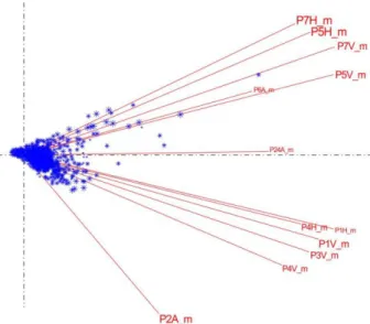
Cartesian (orthogonal) reference system, a biplot visualization is possible only for d 3. Using a parallel coordinate system, the visualization is possible for any d p (Vairinhos & Galindo, 2012). The data illustrated in Figure 4 b) and c), extracted from the cube in Figure 4 a), is named in what follows, respectively by: X (m, n), Y (m, k), Z (k, n). In X (m, n), for a specific equipment, rows represent Observation Points and columns represent Fourier frequencies. This means that each X column contains, for a specific Fourier Frequency w, m amplitudes (one for each observation point), for that frequency, obtained by DFT of vibration signals corresponding to observation points. A X row contains the n amplitudes corresponding to the n Fourier Frequencies of a single spectrogram obtained by DFT performed on the vibration signal at a single observation point. In Y(m, k), for a specific w, rows represent OP and columns represent Equipment. In Z (k, n), for a specific OP, rows represent Equipment and columns FF. For each one of those matrices/slices a biplot is possible since only two of the three kinds of information (Modes) are being related. In our case, for n = 3900 FF; k= 4 generators; m = 13 OP, there are three biplots. For example, Figure 5 shows a biplot corresponding to XT (3900, 13). Points
represent n = 3900 FF and arrows represent the m = 13 observation points.
In these biplots the cosines of angles between the vectors representing variables (in this case the OP) are the correlations between those variables. Biplots show a graphical image of that correlation matrix; in this context, the cosines represent the strength of association between the vibration patterns at distinct OP: the greater the absolute value of those cosines the more similar the vibrations are at those points.
Figure 5. HJ-Biplot for matrix X, relating n= 3900 Fourier Frequencies with p= 13 Observation Points. ‘*’ Represents a Fourier frequency; Observation points are represented by vectors labeled according with Figure 3. Tag “_m” means that variables were obtained averaging spectrogram replicas. For biplot in Figure 5, the distances between row markers (Fourier frequencies), represent dissimilarities (in terms of signal energy) between the corresponding frequencies (Galindo, 1986).
6. BIPLOT INTERPRETATION FOR VIBRATION ANALYSIS
RESULTS
The reasoning used for VA results interpretation relates the following items: Fourier Frequencies (wi), Observation
Points (Pj), Equipment (Ek) and, for monitoring,
Observations Occasions (Tl). When all that matters is a
global impression of what is going on, the kind of biplot in Figure 5, where rows (FF) are represented by a non-labelled symbol, can be very useful. The general position of these markers (as opposed to the actual frequencies they represent) can be used as reference to detect changes in the future. In the case of Figure 5, biplot represents 13 spectrograms each one with 3900 FF corresponding to GE1, observed at Feb 1st, 2011 in a “good condition”.
In this case the Fourier frequencies were labeled by ‘*’ but they could have been labelled also using their values (FF) or their amplitudes for each one of OP (variables), as shown, in Figure 6 where FF are identified by labels related with their value in Hz.
For HJ biplots, Galindo (1986) used in this work, the angles between rows and columns (FF and OP in our case) can be statistically interpreted as the degree of contribution from the rows to the columns. If, for a specific observation point (P7V, say) some set of frequencies form small angles with that OP, this means that the identified FF have large contributions for the explanation of the vibration pattern
(represented by a spectrogram) at that OP. For example, it can be seen, in Figure 6 that FF labelled 190 and 191 make angles nearly zero (cosines =1) with P7V observation point, the right support of AC generator. That same figure, also shows that the subset of FF = {159, 158, 477, 588, 636, 637, 350, 349, 196, 189, 191, 190} are the major contributors- by this order - for the vibration patterns at OP subset = {P7H, P5H, P7V, P5V} all belonging to the AC generator component, as can be checked from Figure 3.
This means that, in the biplot, it is possible to, literally, “see” and read all the information that matters for VA results interpretation and diagnosis: OP (spectrograms), FF(w´s), amplitude values and the mutual relations between OP and FF, expressed by angles and distances.
Being a bit more specific, in a 2D biplot let w (an FF) and P1 and P2 two OP. All three markers are represented by 2D points in the biplot. For example: w= (5, 6)T , P
1= (15, 3)T, P2= (1, 0)T. The marker w represents a row in the data set (corresponding to a Fourier Frequency) formed by p (p= 13 in our example) amplitudes, the number of observation points. In the same way, the marker P1, for example, represents a vector with n (n=3900 components in our case), a column in the data set, containing the amplitudes of the spectrogram observed at point P1. The same for P2.
The contribution of a Fourier Frequency w to explain the vibration pattern at point P is obtained projecting w on P, by
) ( cos
,P wTP w P
w = = (7)
In the process of VA results interpretation, the four basic tasks are:
Task 1 – Set a reference: specify a biplot for a known reference condition.
Task 2 – Detect a change: compare a measurement with the reference.
Task 3 – Diagnostic: identify possible failure modes. Task 4 –Prognosis: given some trend pattern, predict the failure.
Task 1 (set a reference)
This task corresponds, roughly, to Phase I in the process of specifying a SPC control chart. For a specific equipment, assuming a known condition and the corresponding working parameters, several replicas of vibration measurements are obtained for all OP and for identical machines (same maker and model). The biplots corresponding to the spectrograms of these observations are built and studied, identifying the sets of frequencies that are more important for the characterization of vibration patterns at specific observation points or at homogeneous sub-groups of OP.
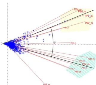
Figure 6. For GE1 in the reference condition, the frequencies that
must contribute to the Motor and Generator form the signaled Co-cluster = {{P7H, P5V, P7V, P5V}, {189, 196,
195, 191, 190}}. FF are represented by blue figures; Variables (OP’s) are represented by red vectors and red
labels. The black lines represent the means both for Generator (G) and Diesel Motor (M) sets of points. For example, in Figure 6, corresponding to an assumed good condition of Generator Number 1 (GE1), two main sub-groups of OP can be identified corresponding accurately with the Diesel Motor (subset M= {P1H, P1V, P2A, P3H, P3V}) and with the Electric Generator (subset G= {P5H, P5V, P6A, P6H, P6V, P7H, P7V}). In this same Figure 6, the FF labels (not to be confused with frequencies in Hz) that, for this specific condition, have more influence on the vibration patterns at subset of OP M, are: {478, 159, 159, 477, 637, 588, 636, 579, 222, 439, 350, 196, 189, 195}. As already seen, the vibration pattern at point P5V is very well explained by Fourier frequencies labelled 189, 196, 195, 191,190 sorted by increasing effect. This means that, for this specific example, output from Task1 is a description/characterization of biplot structure given by two subsets of OP and corresponding lists of Fourier frequencies with greater contribution for identified subsets of OP. The final decision about this reference biplot configuration can be made using, for example, the bootstrap methodology (Nieto, Galindo, Leiva & Vicente-Galindo, 2014). Figure 7 shows four biplots for GE1, GE2, GE3, GE4 in the assumed reference condition, showing, with small variations, the same macrostructure.
same model and maker and assumed in the same condition. Biplots macrostructure are very similar and defined by two subsets of OP: M (for Diesel Motor) and G (for electric Generator) the two means (black lines) which form an angle θ. Task 2 - Detect a condition change
This task is related with a condition change associated with the emergence and incipient development of a failure. If there is a new failure development process, this process must be the cause of a noticeable change in the vibration patterns at OP and, consequently, of noticeable features in the current biplot. As an example, the process could manifest itself through noticeable changes of angles between OP, changes in the lists of contributing frequencies for OP and changes in some of angles between OP and FF. To be useful, this process must occur before any major external evidence of failure occurs. In synthesis: it is assumed that, when there is an assignable cause of change (not attributable only to chance), such as the development of an incipient failure, that must manifest itself in the corresponding geometric relations of markers in biplots, both FF and OP. For an example, figure 8 shows the biplot constructed with the same graphical parameters, resulting from an artificial modification of spectrograms for observation points P1H, and P1V. This new biplot should be
compared with the one presented in Figure 6 for the reference condition resulting from Task 1. Observe that the macro structure of the second biplot – the Observation Points from the two cluster already identified in Figure 6, corresponding to M (Motor) and G (Generator), although very similar, presents noticeable changes in relation to reference Biplot at Figure 6.
Another graphical manifestation of assignable causes of condition change, are the variations of angles between the subset of FF with higher influence on the vibration patterns at some specific subset of OP´s. In addition, it may happen that a specific assignable cause can produce also changes in the lists of FF with higher contributions for the vibration patterns at OP. For example, from Figure 8 the list of FF with more influence over the G set is the same as before but small variations between the angles are noticed.
Another, rough, way to quantify the biplot change resulting from the existence of a latent failure process can be based on the following reasoning:
Figure 8. Modified reference condition biplot after the emergence of an incipient (simulated) failure which manifest itself in the biplot by the position of P1H, now associated to P4V when in the original it was associated to P4H. The two QQ clusters correspond to AC Generator and Diesel Motor. FF are represented by blue markers; Variables
(OP’s) are represented by red vectors and red labels. The black lines represent the means both for Generator (G) and
Diesel Motor (M) sets of points. Generator (down) is “slightly” different from the reference.
If there is an assignable cause that explains the change in vibration pattern at some OP, this means that a new dimension is needed to account for the information associated with this new variability source.
If the reference biplot (assumed to be 2D) explained 100% of the information associated with the Reference Condition, this would mean, for the current biplot, that the two-factorial solution would explain less than 100% of information; the additional information or variability associated to the new variation source should be accounted for by that additional dimension. To represent 100% variability, it would be necessary now to have a higher dimension biplot.
Rule. Generalizing the idea in 2), a rule to detect the presence of an assignable cause of condition change (presence of an incipient or latent failure process) would be: “If the percent of variance (information) explained by the current biplot is less than that explained by the Reference biplot, this means that, eventually, an incipient failure is developing”.
This rule can become more objective bootstrapping SVD results used to construct the current biplot (Nieto et al, 2014), and performing a statistical test using the corresponding “sampling” distribution: the rejection of a reference hypothesis of no-change would sound the alarm for the eventual presence of a latent or incipient failure
process. Another possibility is to use angle θ as a feature to monitor.
Task 3 – Diagnostic. Identify possible failure modes
Having assumed that equipment condition changed (or is changing) it becomes necessary to identify the cause of that change when such cause can be expressed using relations between frequencies and observation points. For example, let the natural frequency of some equipment be f0 Hz. This means that its harmonics hk = k × f0, k= 1, 2…, if combined with a vibrating pattern of some source can create dangerous resonances. From this observation, would result a rule to detect the presence of harmonics hk (or “near harmonics”)
among the frequencies that most contribute (make smaller angles) to some subset of OP in the biplot.
ISO 10816 (2014) and other international norms are important sources of data to construct rules of this kind. The exact nature of a failure cause, and its expression in terms of FF and corresponding amplitudes at OP can only be specified using deep technical knowledge about the specific machine. For example, ball bearings failures generate vibration processes with frequencies related with the geometry of the bearing and the number of balls. The number of balls combined with the rotation speed generate, in the case of several failed balls, vibration effects whose frequency can be calculated using this knowledge (Emerson, 2016). This means that a technical analysis of specific equipment is needed to create rules relating possible failure causes, technical characteristics and frequencies. In general: if the FF that in the current biplot have higher contributions for the vibration patterns of some subset of OP belong to the set of harmonic frequencies that characterise some specific failure, then possibly, that failure is present or is becoming present. Geometrically, in the biplot, this is equivalent to the definition of detection regions, for each OP or relevant subsets of OP such as M or G defined before. The presence of harmonics associated to a specific class of failures in those regions should work as an alarm signal for that failure. Using a more appealing language: if some specific failure is developing, then those regions should “see” the presence of corresponding harmonics. In other words, the biplot should show a “movement” of some frequencies towards those regions, as if the FF subset corresponding to specific failure modes were attracted by those regions.
Task 4 - Prognosis
The monitoring of a system using biplots can be accomplished measuring vibrations at OP for successive occasions (T=1, 2,…,Q) and comparing the successive biplots with the reference one. For each occasion, the relevant features of the current biplot, for example angle θ between sets of points M and G or the % of variance explained by the first two biplot axis, are extracted and used to perform prediction/prognosis based in the corresponding
trends. When the reference condition is defined by a 2D biplot, then for successive biplots the total percent variance accumulated by the two axes (the same for 3D biplots) are compared with the corresponding value for the reference condition.
Figure 9. A time series of biplots for VA monitoring. Biplot for T= 0 correspond to reference condition. For each observation condition (T=1, 2,…, Q) a biplot is produced
and its features extracted.
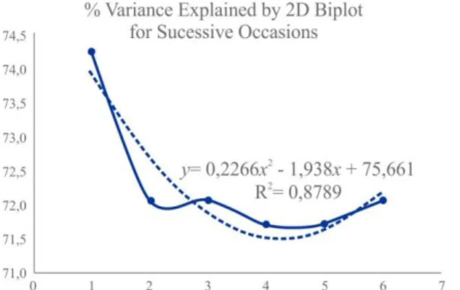
Specifically, for each one of the 5 biplots in Figure 9, constructed with random modifications (bootstrap simulated failures) of reference biplot for GE1, the percent of information/variance explained by those biplots are, for T= 0, …, 5, respectively (74.25, 72.07, 72.07, 71.71, 71.72, 72.07).
Representing these values with a chart (Figure 10), it is shown that, for successive 2D biplots the percentage of information explained is decreasing. This means that the remaining (residual) information/variance, not explained by current biplot, is increasing. This suggests that one additional dimension is needed to account for that unexplained variability and, according with what was explained before, an incipient failure is developping.
Figure 10. Plot and trendline for percent variance explained by successive 2D biplots corresponding to simulated failure data for 6 occasions, showing the need of a third dimension.
Discussion
The present work was based on about 2 GB of observational real data collected from real machines in real operating conditions. This was not enough to identify all possible problems and to check all the nuances and limitations of the
proposed methodology. Further efforts in this direction are needed, but the results obtained so far are very encouraging. To fully explore the ideas proposed in this paper the software to be used must be “tailor-made”: allow dynamic interactions, have the statistical functionality needed to implement the interpretation rules suggested and to give the answers expected in VA. In our case a general-purpose software was used with the consequent limitations (Vairinhos, 2003).
Biplots features extraction, the base of effective comparisons and trend studies implicit in Tasks 1,2,3,4 must be much more developed in future work, and the same applies to failure rules detection.
7. CONCLUSIONS
A biplot based graphical data driven methodology was proposed to monitor vibrations in the context of CBM maintenance.
The methodology is based on observational data collected by fixed or mobile sensors in operating conditions.
When implemented through dedicated software incorporating specific knowledge about the monitored machines, this methodology can contribute to generalise the use of VA.
REFERENCES
Brockwell, P. J., & Davis, R. A. (1991). Time series: Theory and methods (2nd Edition). Springer Verlag, New York.
Beneke, M., Leemis, L. M., Schelegal, E., & Foote, B. (1988). Spectral analysis in quality control: A control chart based on periodogram. Technometrics, vol. 30(1), pp.63-70.
Benzécri, J. P. et Collaborateurs (1973). L’Analyse des Données. Dunod: Paris.
Emerson (2016). Process management CSI 2140 Machinery HealthTM Analyzer. User Guide.
Ferrer, Alberto (2014). Latent structures-based multivariate statistical process control: A paradigm shift. In Quality Engineering, vol. 26, pp. 72-91.
Fokianos, K., & Savvides, A. (2008). On comparing spectral densities. Technometrics, vol. 50(3), 317-331.
Gabriel, K. R. (1971). The biplot graphic display of matrices with application to principal components analysis. Biometrika, vol. 58(3), pp. 453-467.
Galindo, M. P. (1986). Una alternativa de representación simultánea: HJ-BIPLOT. Qüestiió, vol. 10(1), pp. 13-23.
García, D., & Trendafilova, I. (2014). A multivariate data-analysis approach towards vibration data-analysis and vabriation - based damage assessment: Application for determination detection in composite bean. Journal of Sound and Vibration, Vol. 333(25), pp. 7036-7050.
Gower, J. C., & Hand, D. J. (1996). Biplots. monographs on statistics and applied probability, vol. 54. Chapman & Hall: London.
Greenacre, M. J. (2010). Biplots in Practice. Retrieved from http://www.fbbva.es/ ([2017 January 10]).
Halliday, D. M., Rosenberg, J. R., Rigas, A., & Conway, B. A. (2009). A periodogram-based test for weak stationarity and consistency between sections in time series. In Journal of Neuroscience Methods, vol. 180, pp. 138-146.
Jones, Richard H. (1965). A reappraise of the periodogram in spectral analysis”. Technometrics, vol. 7(4), pp. 531-542.
Kolda, T. G., & Sun, J. (2008). Scalable tensor decompositions for multi-aspect data mining. In Data Mining 2008. ICDM’08, Eigtht IEEE International Conference on IEEE, 2008, pp. 363-372.
Kroonenberg, P. M. (2008). Applied multiway data analysis. Wiley: New Jersey.
Li, W., Shi, T., Liao, G., & Yang, S. (2003). Feature extraction and classification of gear faults using principal component analysis. Journal of Quality in Maintenance Engineering, vol. 9(2), pp. 132-143. McSweeney, L. (2006). Comparison of periodogram tests.
Journal of Statistical Computation and Simulation, vol. 76(4), pp. 357-369.
Mendes, S. L. C. M. (2011). Metodos multivariantes para evaluar patrones de estabilidad y cambio desde una perspectiva biplot. Tesis Doctoral. Universidad de Salamanca, España.
Mendes, S., Fernandez-Gomez, M. J., Pereira, M. J., Azeiteiro, U. M., & Galindo-Villardon, M. P. (2012), An empirical comparison of canonical correspondence analysis and atatico in the identification of spatio-temporal ecological relationships. Journal of Applied Statisticas, vol. 39(5).
Nieto, A. B., Galindo, M.P., Leiva, V., & Vicente-Galindo, P. (2014). A methodology for biplots based on bootstrapping with R. Revista Colombiana de Estadística, Current Topics in Statistical Graphics Diciembre 2014, vol. 37(2), pp. 367-397. Retrieved from http://dx.doi.org/10.15446/rce.v37n2spe.47944 ([2017 January 10]).
Papalexakis, E. E., & Faloutsos, C. (2015). Fast efficient and scalable core consistency diagnostics for the parafac decomposition for big sparse tensors. In Acoustics, Speech and Signal Processing LICASSP, 2015 IEEE International Conference on IEE.
Priestley, M.B. (1981). Spectral analysis and time series. Academic Press: London.
Ravishanker, N., Hosking, J. R. M., & Mukhopadhyay, J. (2010). Spectrum-based comparison of stationary multivariate time series. Methodol Comput Appl Probab 2010, vol. 12, pp. 749-762.
Vairinhos, V. M. (2003). Desarrollo de un sistema para minería de datos basado en los métodos biplot. Tesis Doctoral. Universidad de Salamanca (USAL), España. Vairinhos, V. M., & Galindo, M. P. (2012). Biplots
cilíndricos. Joclad 2012, XIX Jornadas de Classificação e Análise de Dados, pp. 132, Março 28-31, Tomar, Portugal.
Zhan, Y., Makis, V., & Jardine, A. K. S. (2003). Adaptive model for vibration monitoring of rotating machinery subject to random deterioration. Journal of Quality in Maintenance Engineering, vol. 9(4), pp. 351-375. ISO 10816-3:2009 (2014). Mechanical vibration. Evaluation
of machine vibration by measurements on non-rotating parts. Part 3, ISO Standards.