The evolution of the OECD countries after the 2008 financial crisis : simultaneous data analysis of the “how’s life” datasets between 2009 and 2015

The evolution of the OECD countries after the

2008 financial crisis

João Pedro Pires dos Reis Muralha Delgado

Simultaneous data analysis of the “How’s Life”

datasets between 2009 and 2015

PROJECT

Dissertation report presented as a partial requirement for

obtaining the Master’s degree in Information Management

MEGI

201

i

NOVA Information Management School

Instituto Superior de Estatística e Gestão de Informação

THE EVOLUTION OF THE OECD COUNTRIES AFTER THE 2008 FINANCIAL CRISIS

SIMULTANEOUS DATA ANALYSIS OF THE “HOW’S LIFE” DATASETS BETWEEN 2009 - 2015

by

João Pedro Pires dos Reis Muralha Delgado

Dissertation report presented as a partial requirement for obtaining the Master’s degree in Information Management, with specialization in Knowledge Management and Business Intelligence

Advisor: Professor Paulo Jorge Mota de Pinho Gomes

iii

DEDICATION

iv

ACKNOWLEDGMENTS

v

ABSTRACT

The financial crisis of 2008 affected virtually every country in the World due to the connectivity of the global markets. Despite the significant contrasts in the starting points, there is the common perception that different economies recovered at distinct paces at least in part due to the policies and methods adopted by the authorities to address the financial crisis. In this context, the OECD “How’s Life” datasets were analyzed with the objective of trying to detect trajectories in countries that could partially be explained by the macroeconomic measures adopted after the crisis. With the support of the OECD secondary data for the period 2009-2015, this novel study involved not only univariate, bivariate, and cluster evaluations but also a three-way data analysis based on the STATIS method. Among the existing multivariate methodologies, STATIS is the most comprehensive and flexible method to assess the evolution of a large (and possibly varying) number of individuals and variables over several years. With the identification of country trajectories in association with the evolution of variables, the findings may be relevant for business organizations with regard to defining strategic directions and making operational decisions.

KEYWORDS

PCA;

Three-Way Data Analysis; STATIS;

vi

INDEX

1.

Introduction ... 1

1.1.

Background and Problem Identification... 1

1.2.

Study Objectives ... 2

1.3.

Study Relevance and Importance ... 3

1.4.

Data Sources ... 3

2.

Literature review ... 5

2.1.

Global Financial Crisis ... 5

2.2.

Government Policies ... 5

2.3.

Economic Models ... 5

2.4.

National Stimulus ... 6

2.5.

Three-Way Data Models ... 7

3.

Methodology ... 8

3.1.

PCA and DPCA ... 9

3.2.

PCA Generalizations ... 10

3.3.

FCA and MFA ... 11

3.4.

STATIS ... 12

3.4.1.

Interstructure ... 13

3.4.2.

Compromise ... 14

3.4.3.

Intrastructure ... 15

3.4.4.

Trajectories ... 15

3.5.

STATIS Variations ... 15

3.6.

MTSA ... 16

3.7.

Techniques Comparison ... 16

3.8.

Clustering ... 17

3.9.

Statistical and Distribution Analysis ... 18

4.

Results and discussion ... 19

4.1.

Data Description ... 19

4.2.

Global Analysis ... 20

4.3.

STATIS Analysis ... 24

4.3.1.

Interstructure ... 24

4.3.2.

Compromise ... 25

4.3.3.

Intrastructure ... 27

4.3.4.

Trajectories ... 28

vii

4.4.

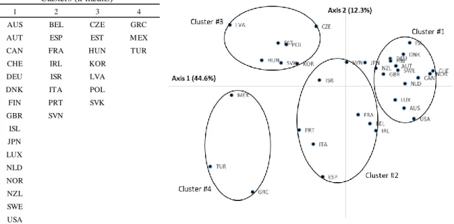
Cluster Analysis ... 30

4.5.

Statistical and Distribution Analysis ... 30

4.6.

Variables Evolution per Country ... 31

4.6.1.

Variable Perspective ... 32

4.6.2.

Country Perspective ... 34

5.

Conclusions ... 37

6.

Limitations and recommendations for future works ... 39

7.

Bibliography ... 40

8.

Appendix ... 44

8.1.

Appendix 1 ... 44

8.2.

Appendix 1 (cont.) ... 45

9.

Annexes ... 46

9.1.

Variables Variation on First Two Axes ... 46

9.2.

Variables Trajectories ... 47

9.3.

Countries Trajectories ... 48

9.4.

Compromise Positions ... 49

9.5.

OECD "How’s Life" Data & Descriptive Statistics - 2009 ... 50

9.6.

Boxplots and Scattergrams - 2009 ... 51

9.7.

Boxplots and Scattergrams – 2009 (cont.) ... 52

9.8.

Histograms – 2009 ... 53

9.9.

Clustering Analysis – 2009 ... 54

9.10.

OECD "How’s Life" Data & Descriptive Statistics - 2010 ... 55

9.11.

Boxplots and Scattergrams - 2010 ... 56

9.12.

Boxplots and Scattergrams – 2010 (cont.) ... 57

9.13.

Histograms – 2010 ... 58

9.14.

Clustering Analysis – 2010 ... 59

9.15.

OECD "How’s Life" Data & Descriptive Statistics - 2011 ... 60

9.16.

Boxplots and Scattergrams - 2011 ... 61

9.17.

Boxplots and Scattergrams – 2011 (cont.) ... 62

9.18.

Histograms – 2011 ... 63

9.19.

Clustering Analysis – 2011 ... 64

9.20.

OECD "How’s Life" Data & Descriptive Statistics - 2012 ... 65

9.21.

Boxplots and Scattergrams - 2012 ... 66

9.22.

Boxplots and Scattergrams – 2012 (cont.) ... 67

viii

9.24.

Clustering Analysis – 2012 ... 69

9.25.

OECD "How’s Life" Data & Descriptive Statistics - 2013 ... 70

9.26.

Boxplots and Scattergrams - 2013 ... 71

9.27.

Boxplots and Scattergrams – 2013 (cont.) ... 72

9.28.

Histograms – 2013 ... 73

9.29.

Clustering Analysis – 2013 ... 74

9.30.

OECD "How’s Life" Data & Descriptive Statistics - 2014 ... 75

9.31.

Boxplots and Scattergrams - 2014 ... 76

9.32.

Boxplots and Scattergrams – 2014 (cont.) ... 77

9.33.

Histograms – 2014 ... 78

9.34.

Clustering Analysis – 2014 ... 79

9.35.

OECD "How’s Life" Data & Descriptive Statistics - 2015 ... 80

9.36.

Boxplots and Scattergrams - 2015 ... 81

9.37.

Boxplots and Scattergrams – 2015 (cont.) ... 82

9.38.

Histograms – 2015 ... 83

9.39.

Clustering Analysis – 2015 ... 84

9.40.

Variables Evolution per Country – Australia and Austria ... 85

9.41.

Variables Evolution per Country – Belgium and Canada ... 86

9.42.

Variables Evolution per Country – Switzerland and Czech Republic ... 87

9.43.

Variables Evolution per Country – Germany and Denmark ... 88

9.44.

Variables Evolution per Country – Spain and Estonia... 89

9.45.

Variables Evolution per Country – Finland and France ... 90

9.46.

Variables Evolution per Country – Great Britain and Greece ... 91

9.47.

Variables Evolution per Country – Hungary and Ireland ... 92

9.48.

Variables Evolution per Country – Iceland and Israel ... 93

9.49.

Variables Evolution per Country – Italy and Japan ... 94

9.50.

Variables Evolution per Country – Korea and Luxembourg ... 95

9.51.

Variables Evolution per Country – Latvia and Mexico ... 96

9.52.

Variables Evolution per Country – Netherlands and Norway ... 97

9.53.

Variables Evolution per Country – New Zealand and Poland ... 98

9.54.

Variables Evolution per Country – Portugal and Slovakia ... 99

9.55.

Variables Evolution per Country – Slovenia and Sweden ... 100

9.56.

Variables Evolution per Country – Turkey and USA... 101

9.57.

Variables Evolution per Country – Table 1 ... 102

ix

9.59.

Variables Evolution per Country – Table 3 ... 104

9.60.

General Trend of Each Variable Per Dimension and Country ... 105

9.61.

Number of Variables with Up/Down Trend Per Axis and Dimension ... 106

9.62.

Country Groups Based on Up/Down Trend of Variables per Axis ... 107

9.63.

List of Countries ... 108

9.64.

Description of Study Variables ... 109

x

LIST OF FIGURES

Figure 2.1 – OECD (2009): The size of fiscal packages (revenue and spending measures) ... 6

Figure 2.2 – OECD (2009): Government investment in stimulus packages in 2008-2010 ... 7

Figure 4.1 – Global analysis: Eigenvalues and variability ... 20

Figure 4.2 – Guttman effect: Observations on the first plan ... 22

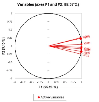
Figure 4.3 – Variables on the correlation circle and oppositions ... 22

Figure 4.4 – Variables variation based on correlations between variables and factors ... 23

Figure 4.5 – Interstructure results ... 24

Figure 4.6 – Compromise positions ... 27

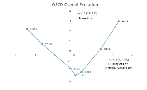
Figure 4.7 – Noticeable country trajectories ... 28

xi

LIST OF TABLES

Table 4.1 – Global analysis: PCA results ... 20

Table 4.2 – First plan: Observations coordinates and contributions ... 21

Table 4.3 – Variables coordinates and correlations ... 21

Table 4.4 – S and RV diagonalization ... 24

Table 4.5 – WD diagonalization ... 25

Table 4.6 – Variables opposition on axis 1 ... 26

Table 4.7 – Variables opposition on axis 2 ... 26

Table 4.8 – Behavior of variables for the long-trajectory countries in clusters ... 33

xii

LIST OF ABBREVIATIONS AND ACRONYMS

CTA Absolute Contribution CTR Relative Contribution

DPCA Double Principal Component Analysis

FCA Factorial Correspondence Analysis GDP Gross Domestic Product

ISI International Statistical Institution MCA Multiple Correspondence Analysis MFA Multiple Factorial Analysis

MTSA Multivariate Time-Series Analysis

OECD Organization for Economic Cooperation and Development

PCA Principal Component Analysis

PESTEL Political, Economic, Social, Technological, Environmental, and Legal STATIS Structuration des Tableaux A Trois Indices de la Statistique

SWOT Strengths, Weaknesses, Opportunities, and Threats

1

1. INTRODUCTION

Although the financial crisis of 2008 was not an entire surprise for people from within the industry with a critical mindset, the reality is that the large majority of the insiders and outsiders perceived the developments as a “Black Swan”: something totally unpredictable and thus, unavoidable. Regardless of the differences in perspectives, the 2008 crisis started in the USA but quickly propagated and contaminated not only the European but also the Asian markets due to the global connectivity and scale of the financial and business operations (Crotty, 2009; Erkens, Hung, & Matos, 2012; Taleb, 2007).

The global financial crisis affected several countries in different ways and to varying extents. Furthermore, the impacted countries were in different positions in terms of macroeconomic aspects among other dimensions, which resulted in a multitude of different starting points for the post-crisis recovery. Nonetheless, the analysis of the growth path of the OECD countries based on the “How’s Life” datasets unveiled a number of distinct progressions associated to the different evolution of variables dependent on the policies adopted by governments and authorities to address the critical financial circumstances (Boarini, Murtin, & Schreyer, 2015; Naudé, 2009; Reinhart, & Rogoff, 2009). The identification of different recovery trajectories and variables’ evolution may provide valuable information for the processes of business decision-making. In fact, the insights resulting from the multivariate analysis of the OECD datasets over time can provide indications in support of efficient decisions related to business strategies and operations. Moreover, the recognition of the insights associated with different approaches might permit to not only adopt the most appropriate methods at an organization level, but also target the most promising countries and geographies for expansion and achievement of the required returns on investments (Clench-Aas, & Holte, 2017; Helliwell, 2003; Krishnamurthy, & Vissing-Jorgensen, 2011).

1.1.

B

P

I

At the request of the President of France in 2010, a team led by Joseph Stiglitz produced a report on the measurement of social and economic progress. This seminal paper represented a breakthrough in relation to the traditional and common way of gauging progress based on GDP alone, which reinforced the OECD initiative related to the collection of data associated to multiple types of variables linked to the quality and conditions of life. Since 2005, the OECD “How’s Life” program has been gathering data and information in relation to the member countries (currently 35) and some partner countries (some six at the moment) (OECD, 2017; Stiglitz, Sen, & Fitoussi, 2010; Yılmaz, 2017).

From 2011 onwards, the “How’s Life” program has been supporting the “Better Life Index” initiative that permits the individual weighting of the different variables to generate results that are tailored to meet the priorities of each user. Although the OECD approach permits to depart from a narrow and limited GDP perspective as discussed by a variety of authors in several papers, the evolution of the multiple variables in the 35 member countries (plus six partners) allows producing a space analysis over time. In addition to a global and intra-country assessment, a multivariate three-way data analysis provides trajectories for the evolution of the various OECD countries in the context of the selected variables (Abdi, & Valentin, 2007; Dolan, Peasgood, & White, 2008; Durand, 2015).

2 The available OECD data relates to the current well-being variables (25) in the period from 2005 to 2015 (or 2016 in some cases) but presents several gaps for a few countries and in some years. This secondary data is credible, consistent, and reliable which permits to have confidence in the results obtained through a multivariate spatial analysis. Even though the OECD “How’s Life” reports are frequently used as an important reference for the 11 covered dimensions of well-being, the datasets permit to develop a multivariate analysis at three dimensions in order to characterize the evolution of the current well-being variables and assess the recovery of the countries after the 2008 crisis (Dazy, Le Barzic, Saporta, & Lavallard, 1996; Veneri, & Murtin, 2016).

1.2.

S

O

The objective of this study is to produce a multivariate three-way analysis of the OECD “How’s Life” data related to most of the member countries in the period from 2009 to 2015. This innovative approach permits the identification of some trends and patterns among the countries as the result of the well-being variables in the aftermath of the financial crisis. The progress and recovery of the countries are initially assessed based on univariate, bivariate, and cluster analysis. However, these methods do not permit to obtain an integrated perspective given the fairly large number of involved countries, variables, and years (Abdi, Williams, Valentin, & Bennani‐Dosse, 2012; OECD, 2014). Likewise, the study discusses the existing multivariate methods in order to justify the STATIS method as the preferred choice for this sort of statistical analysis. In fact, the STATIS method is a comprehensive technique that permits the simultaneous analysis of several data tables through a number of steps: interstructure (for the global tables), compromise (with weights based on the variations of the individual distance), intrastructure (from the principal components for the compromise table), and trajectories (for the individuals). This method was developed by l'Hermier des Plantes under the supervision of Yves Escoufier and is flexible to variations on the number of variables or the number of individuals over time (Dazy, Le Barzic, Saporta, & Lavallard, 1996; Des Plantes, 1976; Escoufier, 1987; Lavit, 1988).

From a business perspective, the results of the STATIS method complemented by the univariate, bivariate, and cluster analysis reveal some patterns and evolving trends in the OECD countries. In the context of different starting points, the various trajectories are partially associated with distinct macroeconomic and financial policies which might provide insights for business decisions. With this information, an organization may decide to focus its efforts and investments in geographies that will be more promising in terms of achieving its strategic goals and obtaining the aspired financial returns (Allin, & Hand, 2015; Chaya, Perez-Hugalde, Judez, Wee, & Guinard, 2004; Teece, 2010).

Overall, the main goal of the study is the identification of countries with a differentiated evolution since the 2008 financial crisis. As the impact of the crisis was experienced at a global scale, a three-way data analysis reveals the countries with different recovery patterns given the impact of the adopted policies and measures on the well-being variables. In the context of its business values and objectives, an organization should be able to select and implement the policies that match its mission and goals while targeting the countries and regions that will permit to obtain the aspired results (Bénasséni, & Dosse, 2012; Helliwell, 2006; Kroonenberg, 1997).

3

1.3.

S

R

I

To the best of the author’s awareness, the integrated and three-way analysis of the OECD “How’s Life” datasets over time (from 2009 to 2015) has not been produced before and so, there are a gap and an opportunity in terms of expanding the existing knowledge. The study helps to clarify the differences in the recovery paces of the various OECD countries and identify some of the possible underlying reasons associated to the selected well-being variables (Dazy, Le Barzic, Saporta, & Lavallard, 1996; OECD, 2017).

In addition, the study analysis might provide useful insights and perspectives for businesses that are considering the possibility of either initiating or expanding their operations in overseas markets. Although the study is not conclusive in all possible aspects and relevant dimensions, the outcome of the study may provide beneficial and interesting indications to organizations in relation to not only creating knowledge and having an additional lens to access international markets and opportunities but also providing some signs in relation to the most desirable internal policies and decision criteria (Hill, 2008; Kotter, 1996).

As such, the STATIS analysis of the OECD countries’ evolution since 2009 supports the creation of a new perspective with the potential to be applied in practice. Moreover, the study attempts to build on the existing data and knowledge, which represents a contribution to move away from the mainly intuitive expectations and perceptions while reinforcing, challenging, or complementing the available reports and indicators. With the obtained views regarding the impact of more forward or restrictive policies on relevant variables, it might be possible to achieve some indications for the benefit of business organizations (Abdi, Williams, Valentin, & Bennani‐Dosse, 2012; Stiglitz, Sen, & Fitoussi, 2010; Veneri, & Murtin, 2016).

1.4.

D

S

As discussed, the overriding purpose of the study is the generation of additional insights in relation to the OECD datasets to support the senior management decision-making processes, namely in terms of international operations and even the implementation of certain degrees of change (e.g., policies, methods, and criteria) within an organization. The new information results primarily from the application of the STATIS model to most of the OECD “How’s Life” datasets in the period from 2009 to 2015 (seven years). At this stage, it is not considered necessary to enter in a marketing research process which is a limitation of the study that can be addressed in the future (Dazy, Le Barzic, Saporta, & Lavallard, 1996; Hill, 2008; OECD, 2017).

In this context, the study employs quantitative secondary data that was originally produced for a different (but connected) purpose. Although the latest set of the OECD data (in the 2017 report) relates to 2015, the source of data is reliable and credible and therefore, the datasets can be used in a dependable and consistent way. The source of data is obviously external and the numeric data was obtained through the OECD published materials (namely reports and websites). At this stage, there is no need to employ a descriptive or casual research (Helliwell, 2003; OECD, 2017).

Moreover, the study uses an exploratory research designed to discover tentative insights (based on the variable relationships) in a flexible way that might prompt further research in the future. With regard to data preparation and analysis, the study employs a multivariate technique in complement

4 to univariate, bivariate, and cluster analysis techniques as previously described. The study presents the main findings and results alongside the identification of the areas for further work, investigation, and possible research (Bénasséni, & Dosse, 2012; Kroonenberg, 1997). A summary of the study was submitted as a contributed paper for the biannual WSC (World Statistic Congress) of ISI (International Statistical Institute) that is going to be held in Malaysia during August 2019 (ISI, 2018).

5

2. LITERATURE REVIEW

2.1. G

F

C

The global financial crisis of 2008 was perhaps the worst financial crisis since the Great Depression of the 1930s. The crisis started with defaults in the USA subprime mortgage market in 2007 and grew into a global banking crisis due to excessive risk-taking that magnified the financial impact in a highly interconnected global industry. With the collapse of the investment bank Lehman Brothers in September 2008, the central banks (namely the Federal Reserve and the European Central Bank) had to implement a large bail-out program addressed at many financial organizations in combination with extensive monetary and fiscal policies to avoid the probable collapse of the global financial system. The combination of the USA crisis with the European debt crisis shortly afterwards resulted in a large downturn and recession of the global economy in association with severe restrictions imposed in the banking system from 2009 onwards (Blanchard, 2009; Crotty, 2009; Havemann, 2009; Rudd, 2009; Taylor, 2009; Verick & Islam 2010).

2.2. G

P

In this context, the investors and families had justified fears of a major global recession that were addressed by the macroeconomic policies implemented in many countries, such as vast monetary easing through major cuts in interest rates and quantitative easing. Apart from programs of extensive fiscal stimulus in some countries, it was necessary to not only bail-out the private financial institutions but also implement the nationalization of some banks. These policies of extremely low interest rates and large quantitative easing conducted to private debt, increasing real estate prices, growth in commodities consumption, and preservation of economically unviable industries. As an almost unavoidable consequence, many countries experienced a surge in fiscal deficits and national debts which conducted to difficulties related to sustainability and restrictions in combination with challenges regarding the reversion of nationalizations and even ethical behaviors (Blanchard, Akerlof, Romer & Stiglitz, 2014; Brumby & Verhoeven, 2010; Claessens, Dell’Ariccia, Igan, & Laeven, 2010; Eubanks, 2010; Litan, 2012; OECD, 2009; Reinhart & Rogoff, 2009; Taylor, 2013).

2.3. E

M

Among other economic theories, there are two contrasting perspectives (Keynesian and Austrian) on the roles and policies to be adopted by a government in particular during a crisis. In essence, the Keynesian views advocate that the private sector conducts to inefficiencies and so, the governments must intervene through active monetary policies implemented by the central banks. However, the designated Austrian school argues that the governments should have a limited intervention (mainly related to private property and individual rights) and should use the gold standard in order to avoid large volatility cycles resulting from the artificial stimulus. Despite the Austrian calls for a self-correction of the markets, the governments initially adopted a Keynesian approach in terms of lowering interest rates and injecting money (in addition to public spending and labor-intensive investments) to stimulate the economy, maintain demand, and bail-out the private sector which was followed by austerity measures and public/private deficit reductions (plus banking regulations and structural competitive reforms) that are perhaps more in line with the Austrian school (Maurel & Schnabl, 2012; Snowdon, Vane & Wynarczyk, 1994).

6

2.4. N

S

In accordance with the OECD, most governments implemented economic stimulus packages after the 2008 crisis to raise not only short-term demand but also supply and innovation. In particular, the stimulus packages targeted (1) modern infrastructure, (2) research and development, (3) innovation, (4) small to medium enterprises, (5) education, and (6) green technologies to create growth and achieve the long-term objectives. With regard to the sizes and features of the packages, the fiscal initiatives in the OECD countries during the initial three years represented some 3.5% on average of the 2008 GDP of those countries but with significant differences at country level (ranging from 0.1% to 5%). The countries with the largest fiscal packages were Australia, Canada, Germany, Japan, Korea, New Zealand, Spain, and the United States while Hungary, Iceland, and Ireland were even increasing the fiscal positions immediately after the subprime crisis (OECD, 2009).

Figure 2.1 – OECD (2009): The size of fiscal packages (revenue and spending measures) Although most countries have implemented tax adjustments and investment programs, the countries that favored investments over taxation were mainly Japan, France, Australia, Denmark, and Mexico. In particular, Australia, Poland, Canada, and Mexico anticipated more significantly the public spending but Denmark, France, and Japan also presented a clear focus in this regard. There was widespread support to households and the Czech Republic, Japan, Korea, Portugal, Mexico, and Slovak Republic also provided assistance to some businesses. Apart from financial measures (such as bail-outs), there was a need to inject liquidity in the economy and protect employment through the packages that stimulated short-term demand but, in addition, the various governments presented varying degrees of focus on the supply side with longer-term objectives in mind (OECD, 2009).

So, the initiatives of the various governments related to (i) measures to protect the banking system, (ii) policies to support businesses through tax reductions, credit guarantees, reductions of labor costs, and employment incentives, (iii) protection of some sectors (e.g., banking and construction),

7 and (iv) help to families and households based on tax reduction, cash payouts, unemployment subsidies, and low health costs. Last but not least, the different countries implemented (v) programs (i.e., stimulus packages in line with the Appendix 1) targeting innovation and long-term growth such as infrastructures, research and development, human investments, green technologies, innovation, and entrepreneurship with the clearly stated objective of coming out stronger from the crisis and being more competitive and prosperous afterwards (OECD, 2009).

Figure 2.2 – OECD (2009): Government investment in stimulus packages in 2008-2010

2.5. T

-W

D

M

Apart from the literature and papers on the circumstances surrounding the 2008 financial crisis and the policies implemented by the governments of the various countries, the literature review addressed not only the OECD “How’s Life” program and circumstances, but also the simultaneous analysis of datasets. With a clear focus on the implementation of the STATIS method, the revision of the literature related to models for the analysis of three-way data (addressed in section 3.) covered an extensive range of techniques that included PCA and DCPA (plus generalizations), FCA and MFA, and MTSA in complement to STATIS (and related variations) in order to assess the merits and benefits of each method for multivariate analysis. The review was produced with the ultimate objective of analyzing the OECD countries’ evolution in the context of the different variables and national policies implemented during the aftermath of the global financial crisis (Abdi, Williams, Valentin, & Bennani‐Dosse, 2012; Allin, & Hand, 2015; Benzécri, 1992; Clench-Aas, & Holte, 2017; Dazy, Le Barzic, Saporta, & Lavallard, 1996; Escoufier, 1987; Kroonenberg, 1997; OECD, 2017).

8

3. METHODOLOGY

With the objective of assessing the evolution of the OECD countries after the 2008 global financial crisis, the “How’s Life” data tables were analyzed based on the STATIS method. However, there are several other methods for the joint analysis of multiple data tables as discussed in the following subsections. In addition to the STATIS study, the set of data tables was initially evaluated based on a cluster analysis complemented by a univariate and bivariate assessment.

The study of the OECD “How’s Life” data tables during the period between 2009 and 2015 involved a three-way data analysis. With application to many different sectors and fields of activity, the method was created by Tucker for application to psychology data with the development of models (i.e., three-mode components and factor analysis) and algorithms to estimate the involved parameters. This work has been progressively expanded by other authors to multidimensional scaling, multi-sample common PCA, STATIS technique, three-mode clustering, constrained three-way analysis, three-way contingency tables, and three-way variance analysis among other techniques.

The main classes of data are profile data (most common), similarity data (relevant for certain fields), and preference data (seldom used due to issues with analysis) which can be derived to obtain means, covariances, frequencies, etc. Data can have a dependence structure (with profile data being split into groups to predict certain variables) or an interdependence structure (to study the relations among variables). In addition, three-mode data involves three types of entities (including time, for instance) while multiple-set data are usually two-mode three-way data (cross-product matrices, covariance matrices, etc.) derived from raw data that cannot be analyzed in its initial form (i.e., it requires a pre-analytical transformation).

In terms of three-way methods, the data-analytic techniques address populations and identify individual differences, unlike the stochastic frameworks that rely on distribution assumptions. The modeling techniques either model directly the three-way data or model indirectly with the view of fitting multi-set data into derived three-way matrices (covariance, correlation, and cross-product among others).

For profile data, the dependence techniques are general linear models (two-block multiple regressions, three-mode redundancy analysis), interdependence techniques are components methods (three-mode component analysis, parallel factor analysis, three-mode correspondent analysis, latent class analysis, spatial evolution analysis), mixed techniques (multi-set canonical correlation analysis, procrustes analysis, multi-set discriminant analysis), and clustering methods (three-way mixture method).

There are also covariance models for profile data, namely the stochastic covariance models (invariant factor analysis, three-mode common factor analysis, additive and multiplicative modeling of multivariate and multi-occasion matrices, simultaneous factor analysis) and exploratory covariance model methods (three-mode component analysis, simultaneous component analysis, indirect fitting with component analysis).

With regard to similarity and preference data, it is possible to employ multidimensional scaling models (individual differences scaling, general Euclidean models, three-way multidimensional

9 scaling), clustering methods (individual differences clustering, three-way ultra-metric trees, synthesized clustering), and unfolding models (three-way unfolding).

3.1.

PCA

DPCA

The purpose of PCA (principal component analysis) is to present the information contained in large data tables of variables related to individuals in a graphic way. Although the theoretical concepts of this essentially descriptive method are not recent, the current computing capabilities permit to fully benefit from this statistical method. With application to numeric data in many different areas, a PCA study unveils the structure involved with the system of variables in terms of associations and oppositions while revealing the existing groups of individuals/objects relative to the considered variables.

The PCA method is applied to tables Xo with n individuals and p variables and data of different type

(continuous, discrete, or ordinal). The lines are the vectors of individuals while the columns are the vectors of variables. To obtain the “distances” between variables, it is necessary to attribute a defined weight to each individual (weights matrix D) and ensure that the sum of weights is equal to one. Moreover, the center of gravity (g) is a vector obtained by applying the weights matrix to the data table to obtain the weighted average of the individuals for each variable (g=XoD1n). With this

information, it is possible to obtain the centered data table X and, if necessary, also the standardized data table through Xs=X(diagV)-1/2, with V being the variance and covariance matrix (V=tXDX) while R

is the correlations matrix (R=t_X

sDXs) and summarizes the structure of linear dependence among the

variables.

With regard to the individuals, it is necessary to define a metric Q for the space in order to calculate the distances between individuals. The most common metrics tend to be either Q=Ip or, in case of

standardization, Q=(diagV)-1 _{and the cluster inertia I}

g is either equal to the sum of the variance of the

variables (for Q=Ip) or equal to p (for standardized variables). As the metric for the variables space is

the matrix D, the study of a data table is characterized by the set of matrices (X,Q,D) and the associated object W=XQXt _{or V=}t_XDX.

The objective of the method is to obtain a similar representation of the individuals’ cluster on a sub-space of lower dimensionality (i.e., q<p) which involves the least possible deformation of the projected distances and thus, the maximization of the projected cluster inertia. In this context, the sub-space of q dimension is defined by the q orthogonal eigenvectors k of VQ associated to the

largest q eigenvalues k whose sum equals the retained inertia (from VQ k= k k). In addition to the

principal axes k of inertia, the associated principal factors are obtained through zk=Q k (from

QVzk= kzk) and the orthogonal principal components result from Yk=XQ k=Xzk. (i.e., the principal

components are a linear combination of the initial centered variables).

So, the principal components are variables with zero mean and uncorrelated, have variances equal to the associated eigenvalues, and permit a reduction in dimensionality in the interest of interpretation. The decision on the number of q principal components to be selected results from a combination of criteria: Pearson (retain at least 80% of the total inertia), break-point in the plot of eigenvalues (scree plot), and Kaiser (retain at least the eigenvalues above the average value). In the case of standardized data, the diagonalization of R provides vectors with coordinates that represent the loadings to generate the principal components.

10 To interpret the axes, the correlations between the principal components and the variables of the initial tables are represented in correlation circles which permits to infer the main aspects associated with each axis. The absolute and relative contributions of individuals and variables in relation to the principal components permit to identify the individuals and variables that are relevant for the interpretation of axes (i.e., CTA above average) and well represented (i.e., CTR above 0.5, which is the percentage of inertia associated to individuals or variables explained by each axis).

Once the principal components have been established, it is possible to position supplementary variables and individuals (either additions to the data set, or excluded data to avoid the loss of detail resulting from the standardization process) in the graphic representations. In fact, the coordinate of a supplementary individual represented by the vector on axis k is ⟨ │ ⟩Q = t Q while the

coordinate of a supplementary variable j _{on axis k is obtained through ⟨} j_{│ ⟩}

D = ( j, )

= t

j D

/

A DPCA (double principal component analysis) involves the “cubic” data related to the same variables and same individuals at various moments in time. Although the third dimension can be different from time, the results will probably be difficult to interpret. The objective of DPCA is to compare the evolution of both the variable relations and the individuals through a process with three phases: analysis of the global evolution, study of the data deformations around the centers of gravity, and representation of the individuals’ evolution over time on a common space to be defined.

The global evolution of the individuals (interstructure) is based on the PCA (principal component analysis) of the centers of gravity of the various data tables, which produces the Euclidean image of the tables on a space with the required dimensions. The first axis of this image is usually related to the continuous evolution of the centers of gravity over time. Then, it is possible to center the data to eliminate the previous evolution effect and study (based on the PCAs of the tables) the variations of the individuals around their centers of gravity. The PCAs of the tables can be interpreted based on graphic representations, and provide the principal components as orthogonal axes that permit the definition of a common space for the representation of the individuals.

The third phase of the PCA (intrastructure) results in the identification of a space of reduced dimensionality where it is possible to project and represent the evolution of the individuals over time. Although different methods can be used, the selection of the axes for the representation of the individuals is often based on the maximization of the inertia associated to the projections which involves the selection of the eigenvectors associated to the biggest eigenvalues based on a criteria such as Pearson (>=80%), scree plot (“elbow”), and Kaiser (at least above average). This process involves the PCA of an extended data table with the juxtaposition of the centered initial tables. The trajectories of the individuals are projected on the selected axes which can be interpreted based on their correlation with the compromise position of the variables (correlation circle).

3.2. PCA

G

PCA is a common method to investigate the existing structure in a large data set in order to identify the relationships between the variables. However, there are instances where the data can be classified in various types (or modes) which requires an extension of the standard PCA method. It is

11 possible to address these situations based on a three-mode principal component analysis as an adaptation of the common PCA that introduces significant levels of complexity.

The three-mode PCA (also designated singular value decomposition) is a generalization of the standard PCA that allows identifying the relations between the components of the modes through the simultaneous analysis of the variables and individuals. The interactions between components are captured in a three-mode core matrix that reflects the essential characteristics of the data. The most general three-mode PCA is called Tucker3 (T3) and involves three distinct modes with an unrestricted core matrix. The Tucker2 (T2) model is an alternative model with two unequal modes with an unrestricted extended core matrix.

With the objective of analyzing three-mode data, there are a number of different models that are variations of the Tucker approach. Among the fixed models, there are two classes of component models: models with three-reduced modes (T3, Three-Mode Scaling, PARAFAC1, CANDECOMP, and INDSCAL) and models with two-reduced modes (T2, IDIOSCAL, PARAFAC2, CANDECOMP, and INDSCAL). These models have decreasing levels of generalization, and the most usual technique to solve these models is ALS (alternating least squares).

In brief, the Three-Mode Scaling is similar to T3 but two reduced modes are equal, PARAFAC1 (parallel factor analysis) is the same as CANDECOMP (canonical decomposition) and involves a T3 approach with a three-way identity matrix as the core matrix, IDIOSCAL (individual differences in orientation scaling) is similar to T2 but with the two reduced modes being equal, and INDSCAL (individual differences scaling) is also identical to T2 with the two reduced modes equal and some additional restrictions. Overall, there are methods more adequate for data sets that evolve over time, such as STATIS, MFA, and DPCA.

3.3. FCA

MFA

The FCA (factorial correspondence analysis) method has the objective of identifying the links between two sets of modalities through the graphical display (with lines and columns on the same representation) of the information contained in a table of measurements. An FCA study can be regarded as a particular case of a PCA employing the metric 2 _{to have the proximity between the}

lines and columns. The FCA is essentially a descriptive method to possibly be complemented by a classification, and the data tables suitable for FCA are not only contingency tables but also tables with binary data and positive measurements.

With a contingency data table and the associated frequency table, it is possible to perform two PCAs: one for the cluster of row-profiles and another for the cluster of column-profiles that provide parallel results. In addition, the FCA involves the non-centered PCA of two profile clusters (lines and columns) to obtain the principal factors and principal components. The two analysis conduct to the same eigenvalues between 1 (trivial, to be discarded) and 0 and the principal factors of one of the analysis are proportional to the principal components of the other (transitional formulas). The symmetric results of the two PCAs permit to diagonalize only the matrix of the smallest dimension and use transition formulas to obtain the principal components for the other matrix, and also to overlap the principal plan of the row-profiles and column-profiles to represent simultaneously the categories of the two crossed-variables.

12 Similarly to a PCA, the interpretation of the principal components hinges on the important absolute and relative contributions of the row-profiles and column-profiles. The MCA (multiple correspondence analysis) is an extension of FCA for a number of disjunctive categories (i.e., mutually exclusive) in questionnaires with the interesting property that a number of aspects (e.g., total inertia, mean of eigenvalues, contribution of modalities to total inertia, etc.) are a function of the questionnaire structure (i.e., number of questions and categories).

The MFA (multiple factorial analysis) is suitable to study individuals with a certain number of quantitative or qualitative variable groups that may have been measured at different moments in time or may have resulted from the re-arrangement of variables. The first stage involves the PCA of the different variable groups to obtain the associated eigenvalues and eigenvectors. The first eigenvalues are especially interesting because their inverses are the ponderation factors for the subsequent stages that permit to balance the role of tables during the analysis process.

The next stage (intrastructure) relates to the representation of the individuals in each table on the same space, which is applicable not only to the compromise positions of the individuals but also to the individuals’ trajectories over time. The MFA method permits to weight the variables in order to balance the influence of the various variable groups, which can be affected by the number of variables and table structure. This weight is the same for all variables in the same table and is equal to the inverse of the inertia of the first principal component for the table. In order to represent the compromise position of the individuals, it is necessary to produce a weighted PCA (using the inverse of the square root of the first eigenvalue) of the juxtaposed data tables which provides an average Euclidean image.

In the following stage, it is required to project the various clusters and obtain the trajectories of the individuals which can be achieved by treating the clusters as supplementary elements in relation to the previous PCA. Having a representation of the average individuals and trajectories, it is indispensable to also represent simultaneously the set of variables using the previous global PCA. Then, the interstructure study involves the comparison of the variable groups and their representation on a common space using the first eigenvalues of the variable groups as weights that conduct to norms dependent on the structure of the group.

3.4.

STATIS

The STATIS (Structuration des Tableaux À Trois Indices de la Statistique) method (Escoufier, 1987; Lavit, 1988) permits to analyze cubes of data and obtain a joint assessment of a set of quantitative tables. In particular, this technique is useful for the analysis of data evolution over time and so, it is related to techniques such as DPCA (double principal components) and MFA (multiple factorial analysis). Unlike the more classical and descriptive statistical methods of analysis (e.g., PCA and FCA) focused on a single table and a few variables at a time, the STATIS approach permits to evaluate multiple tables of the same type simultaneously.

The currently available computing capacity allows the analysts to avoid the complexity resulting from the evaluation of each table and variable by employing an integrated graphic representation of the data collected on periodic occasions. The focus on the relative position of the individuals provided by the STATIS analysis results from the graphic displays that summarize the most important aspects related to large data sets involving multiple variables. Despite the loss of some information detail,

13 the representations resulting from a multidimensional method (such as STATIS) are easy to interpret visually which permits to unveil the main features of the data.

For a set of S data tables, the STATIS method represents each study by an object Ws and the study is

defined by three elements (Xs, Qs, D)s with D (observations weight) being constant and with Qs being

equal to either Ip or (diagV)-1 (for normalized data). The joint analysis of multiple data tables permits

to have a varying number of variables (STATIS, for object relations) or objects (Dual-STATIS, for variable relations) over time and to collect data with or without a defined periodicity (or another type of dimension either than time). This sort of method involves four stages:

1. Global analysis based on the study of an interstructure comparing the data table structures with the support of the existing distances and graphic representation;

2. Identification of a compromise table W representing all the data tables in order to avoid the complexity of analyzing the various tables in an independent and separate way;

3. Detailed analysis resulting from the study of the intrastructure which permits to evaluate the similarities and differences between the tables based on their compromise positions;

4. Analysis of the trajectories presented by each component (objects or variables) of the various data tables over time (or relative to another dimension) to appraise the evolution.

3.4.1. Interstructure

As indicated, the interstructure permits an overall comparison of the data tables based on their representations on a plan. This approach requires the creation of an object for each data table, the definition of a metric for distances, and the development of the Euclidean image of the objects based on the distance criteria. For a table Xs (n x p) (with s = 1, …, S), the representative object is obtained

by: Ws = Xs Qs Xts (size n x n) with Qs = (diagV)-1 (covariance from V = Xts D Xs) given the heterogeneity

of the variables’ data and units in the study.

In order to obtain distances between objects and represent the tables in a graphical way, the STATIS method uses the Hilbert-Schmidt inner-product which indicates the existing degree of association between data tables: HS = Tr(DWsDWs’), where Tr (trace) is the sum of the diagonal

elements. Apart from the distances, this inner-product also permits to obtain the squared norm of an object Ws: 2HS = HS = Tr (DWsDWs) = ( i (s))2 where i(s) is the -rank eigenvector of

WsD (with D = Ip ). Moreover, if the norms of the objects Ws are significantly different, it is

necessary to use normalized objects Ws / HS in order to avoid wrong interpretations due to the

dominant effect of the high-normed tables on the compromise. In fact, objects with high values affect the compromise structure and can mislead the interpretation of results.

The Hilbert-Schmidt inner-product provides also the table of inner-products between the study tables (Ws and Ws’): S = SSS’ = HS with s= 1, …, k and s’= 1, …, k (with table size k x k) or

Š = Š SS’ = ⟨ │ ⟩HS = (k x k) for normalized objects Ws / HS and

14 designation RV(S,S’) = ⟨ │ ⟩HS = SSS’ / ( S1/2ss * S1/2s’s’ ). The diagonalization of S and Š permits

to obtain the image of the tables, while the RV coefficients (ranging from 0 to 1, and with RV being equal to Š for normed objects) and allow having the distances between the normalized tables. With a view to obtain the Euclidian image of the objects, it is necessary to produce a PCA (principal component analysis) of matrix S (i.e., the inner-product matrix of the objects) which involves obtaining the eigenvalues and eigenvectors (that generate the Euclidean space) of S , with being the matrix of the weights for each table (i.e., k). The coordinates of the points As associated to the

tables Ws are obtained through Yi, with i andYibeing the eigenvalue and eigenvector of i-rank

associated to matrix S which permits to represent the k objects on the i-principal axis.

In practice, the representation is limited to the two first axes (the principal plan) and provides a graphic display of the relations in the interstructure (without interpreting the axes). The distance between the As points is an approximation of the Hilbert-Schmidt distance between the objects

representing the data tables and so, the proximity of two well-represented points on the first plan indicates the existence of a shared structure for the observations in the tables.

With regard to the Euclidean images, the RV coefficient also represent the cosines between vectors OAs and OAs’ (with origin O) as RV(S,S’) = ⟨ │ ⟩HS = SSS’ / ( S1/2ss * S1/2s’s’ ) =

and so, the smaller the angle the higher the correlation of the tables. Moreover, S is a symmetric matrix with all elements positive and thus, all components of its first eigenvector have the same sign according to the theorem of Frobenius. Likewise, the Euclidean representation of the points As on the

first plane is mainly differentiated by the second axis coordinates because the coordinates on the first axis are all positive and of similar (and large) magnitude (i.e., similar norms and high RVs) in order to ensure the comparison and interpretation of the objects (representing the data tables) based on the plan representation.

So, the analysis of the interstructure permits to verify (without explaining) the existence of structural similarities among the data tables which supports the construction of a compromise table W (with size n x n) as a valid summary of the entire set of the data tables. Depending on the Euclidean representation of the tables, it might be necessary to exclude some structurally distinct tables, use normalized objects, or recognize the inexistence of a common structure because the objects are distinct and present low RV coefficients.

3.4.2. Compromise

The compromise table W is defined as the weighted average of the Ws (or Ws / HS ) objects in

accordance with W = sWs (or W = sWs / HS ) with s = ( s ss ) s Y(s)1 for

Ws objects [ or s = s Y(s)1 for normed objects Ws / HS ] with Y1 being the first eigenvector of

matrix S , Sss = 2HS being the sth diagonal element of matrix S, and s the first eigenvalue of

matrix WsD. In this context, the norm of the compromise is HS = s HS for objects Ws

(or HS = 1 for objects Ws / HS) and W is not only a positive semidefinite matrix (i.e., with all

eigenvalues non-negative) but also centered for the weights of the objects. Overall, the compromise table W is a common structure for the objects and permits a detailed analysis of the data tables

15 through the intrastructure and trajectory phases of the STATIS method. The compromise W is a global summary table that permits to avoid the separate analysis of each data table.

3.4.3. Intrastructure

The intrastructure allows obtaining not only the Euclidean compromise image of each individual (i.e., the mean position in the period of analysis) but also the correlation of the variables with the principal components of the compromise in support of interpreting the position of the objects on the compromise plan. In fact, the compromise Euclidean image of the individuals is a set of points B1, …,

Bn with coordinates on axis k obtained through (WD) Vk , with being the eigenvalues of WD

(size n x n) and Vk the associated eigenvectors (k=1, …, n). With regard to the interpretation of the

individuals’ positions, it is possible to identify the meaning of the axes through the correlations between the principal components of the compromise and the variables of the data tables (providing the variables on each table are not highly correlated and thus, the evolution of the object points are related to the variables), with the coordinate of variable on axis k being obtained with ( , ) D = tVk D .

3.4.4. Trajectories

To assess the differences and evolution at individual level, it is possible to represent the associated trajectories on the Euclidean image of the compromise through (WsD) Vk [or ( WsD) Vk

for normed objects] which is similar to the positioning of supplementary elements and provides the coordinates of points B1s, …, Bns (with s = 1, .., k). The points B1, …, Bn are the equivalent to the

centers of gravity for points B1s, …, Bns, and the trajectories of the objects are usually interpreted for

the first two axes only by taking into account the average evolution (i.e., relative to the plan origin for centered variables).

3.5. STATIS

V

Apart from the Dual-STATIS method for a fixed set of variables and their covariance matrices (instead of the cross-product matrices between observations), there are a few other techniques related to STATIS. Among those variations is X-STATIS (or PTA, partial triadic analysis) which is applicable to data tables with always the same individuals and variables over time. The X-STATIS process is similar to STATIS with two simplifications: the inner-product matrix used for the s weights is obtained from

the initial tables Xr (rather than the Ws tables) and the compromise is the weighted average of the Xr

tables (instead of the Ws). As variations of X-STATIS, STATICO and COSTATIS apply a related approach

to two sets of tables through the combination of co-inertia analysis with X-STATIS (which is also similar to Double-STATIS).

With the integration of covariance or correlation and distance matrices, the COVSTATIS and DISTATIS are three-way extensions of multidimensional scaling. COVSTATIS is used to analyze covariance or correlation tables instead of the tables resulting from STATIS cross-products with attention to the normalization process in case of different units. In addition, it is necessary to ensure that all covariance or correlation matrices have the same origin which requires a double centered process. The DISTATIS approach transforms the distances matrices for the observations into cross-product matrices that are used for the STATIS cross-product process.

16 The CANOSTATIS technique involves groups of observations in multiple tables and for each table is performed a linear discriminant analysis. These distance matrices are used as the input to DISTATIS integration and representation process. Power-STATIS is a more generic approach with particular interest for an X-STATIS situation, and ANISOSTATIS permits to avoid the STATIS restriction of applying the same weight for all variables of a table which requires the identification of the most appropriate values to approximate the compromise map to the set of tables. Another extension of STATIS is the (K+1)-STATIS that studies the relationship of the K tables with an external table base on the existing patterns of similarity between the K tables relative to the additional table.

The Double-STATIS further extends the generalization of (K+1)-STATIS with the objective of obtaining two compromises that are as similar as possible (based on the inner-product of these compromises), which is an approach that has been extended to multiple sets of data matrices. This extension is designed STATIS-4 and involves an interactive process to obtain a compromise for each set of tables and an overall compromise. Finally, STATIS is not only related to other techniques such as GCCA (general canonical correlation analysis), GPA (general Procrustes analysis), and multi-block analysis (MFA, SUM-PCA, consensus PCA, MCA) but also a simplification of INDSCAL (individual differences scaling).

3.6. MTSA

The MTSA (multivariate time-series analysis) is specifically employed to study time-related data in tables with the same individuals and variables. This method is similar to DPCA but adds a variable in each table with the same time value for all individuals. The study of the interstructure is focused on the simultaneous evolution of the time series associated with the variables in order to identify a common polynomial trend. This polynomial expression can be adjusted to the centers of gravity and permits to forecast the evolution of the center of gravity for an additional table.

In addition, the analysis of the intrastructure to obtain the compromise position of the variables and trajectories of the individuals involves the PCA of the juxtaposition of the various data tables adjusted to take into consideration the polynomial trend. The results obtained with this approach tend to be similar to the solutions achieved with DPCA and Dual-STATIS (for not normalized objects) and the existing differences are due to the measurement of the individuals’ position relative to the trend instead of their centers of gravity.

3.7. T

C

Overall, the STATIS and Dual-STATIS methods have more flexibility than DPCA and MTSA in relation to the structure of the data tables, while the MFA is the only approach that permits the inclusion of qualitative variables. In addition, the STATIS, Dual-STATIS, and DPCA methods allow the use of normalized or normalized objects but MFA employs normalized objects and MTSA treats non-normalized objects. With regard to the compromise, the MFA, DPCA, and MTSA techniques take into account the objects that represent each table while the STATIS and Dual-STATIS approaches adopt a linear combination of the objects based on the existing correlations which result in a compromise of the same nature as the objects (i.e., either normalized or non-normalized).

In terms of interstructure, STATIS and MFA provide similar compromise positions of the individuals on the Euclidean space that represent the averages for the period while the trajectories of the

17 individuals are also similar and obtained through projections relative to the intrastructure axes (as supplementary elements) which allow describing the evolution of the data. The methods Dual-STATIS, DPCA, and MTSA provide only the trajectories of individuals which are interpreted based on the compromise positions of the variables, but the average positions of the individuals can be calculated. The intrastructure axes are interpreted based on the correlation with the initial variables (STATIS and MFA) or with the compromise variables (Dual-STATIS, DPCA, and MTSA).

The interstructure is the aspect that most differentiates the various methods. STATIS and Dual-STATIS produce a PCA of the table from the inner-product of representative objects which provides an indication of proximities without allowing to interpret the axes meaning. The MFA projects the representative object on the axes resulting from the intrastructure which provides easier to interpret images but not of the same quality. DPCA and MTSA assess the general trend of the tables through a PCA of the centers of gravity and a polynomial adjustment relative to the centers of gravity.

The various methods employ different processes to evaluate the quality of the individuals’ representations, while MTSA is the only technique that specifically takes into account the time dimension in the interstructure and intrastructure stages of the process. The STATIS solutions are perhaps the most optimized but the interstructure and intrastructure processes do not facilitate the interpretation of results, which does not occur to the same extent with MFA for similar results. DPCA and MTSA appear to have more limitations in terms of their applicability.

3.8. C

Cluster analysis involves the grouping of objects in a way that combines similar objects in the same group (i.e., cluster) while ensuring the groups are as much distinct as possible. This is achieved by ensuring that the total inertia (which is a constant value) is equal to the smallest possible sum of the intraclass inertias (in order to have homogeneous clusters) and so, also the maximum possible sum of the interclass inertias (resulting from to the groups’ centers of gravity). A cluster analysis can be used before a factorial method to reduce complexity or afterward to summarize the obtained results. Among the multiple clustering techniques, it is worth noting the hierarchical clustering and the K-means method of creating groups of objects. The hierarchical approach builds a hierarchy of clusters by progressively identifying pairs of observations or clusters based on a pre-defined similarity criterion which merges all objects (and clusters) in a sequence of new clusters until the complete hierarchy is created. The results can be displayed graphically in a dendrogram with an indication of the links, and the similarities between observations are measured based on a distance criterion (Euclidean, Ward, Manhattan, etc.)

The K-means algorithm allocates all the observations to k clusters based on the distances to the means. The method is randomly initialized with the identification of the initial seeds and the allocation of the observations given the distances to these random seeds. Next, the seeds are replaced by the centers of gravity of the initial clusters and the allocation process is repeated multiple times in an interactive way until a degree of stability is achieved. Despite the good results obtained with K-means, it is not possible to ensure that the best possible clustering result has been achieved, and the algorithm is highly sensitive to outliers.

18

3.9.

S

D

A

As an initial assessment and in complement to the subsequent STATIS and global PCA studies, the statistical and distribution analysis of the data tables permits to obtain not only preliminary insights but also some additional information in relation to the data set. As an illustration, this type of analysis allows the identification of outliers that should be addressed in order to avoid a distortion of the results from the multivariate analysis. In this context, it is indispensable to combine and complement the multivariate statistical study with one and/or two-dimensional descriptive statistics. Likewise, the study takes into consideration some descriptive statistics (minimum, maximum, range, variance, and standard deviation as measures of dispersion; quartiles, median, and mean as measures of central tendency; plus skewness for symmetry, kurtosis for comparison with a normal distribution, and standard error) pertaining to the variables in the annual data tables. Moreover, the analysis is graphical and based on histograms to assess the distribution of the variables’ values, boxplots to explore the structure of the variables data (namely in terms of outliers), and scatter-grams to obtain a unidirectional or bidirectional appreciation of the data. It is necessary to consider the different units of the variables to assess the need for standardization and thus, avoid the dominance of a few variables despite the loss of some detail and information.

With regard to the boxplots, it is worth noting that the outliers can be categorized in moderate or severe outliers based on the distance to the lower (25th _{percentile) or top (75}th _{percentile) quartile}

exceeding either 1.5 (moderate) or 3 (severe) times the inter-quartile range [i.e., Q1 - (1.5 or 3) x IQR or Q3 + (1.5 or 3) x IQR]. Moreover, it is important to keep in mind that the mean values for the various variables in the descriptive statistics are not necessarily the same as the actual means of the variables for the countries of the OECD because the scale factors (such as the population size, among other criteria) are different for distinct variables and are not being taken into account in this study for the sake of preventing excessive complexity.