Increasing the regional availability of the Standardized Precipitation Index: an operational approach

(1)

AbstrAct: The need to use a length of rainfall records of at least 30 years to calculate the Standardized Precipitation Index (SPI) limits its application in several Drought Early Warning Systems of developing countries. Therefore, in order to increase the number of weather stations in which the SPI may be applied, this study quantified the difference among SPI values derived from calibration periods (CP) smaller than 30 years in respect to those computed from the 30-year period of 1985 – 2014 in the State of São Paulo, Brazil (time scales ranging from 1 to 12 months were considered). The correlation, agreement and consistency of SPI values derived from CP ranging from the last 30 to 21 years have been evaluated. The Kolmogorov-Smirnov/Lilliefors test indicated, for all CP, that the 2-parameter gamma distribution may be used to calculate the SPI in

Agrometeorology -

Article

Increasing the regional availability of the

Standardized Precipitation Index: an operational

approach

Monica Cristina Meschiatti*, Gabriel Constantino Blain

Instituto Agronômico - Centro de Ecofisiologia e Biofísica - Campinas (SP), Brazil.

*Corresponding author: monicameschiatti@hotmail.com

Received: Oct. 8, 2015 – Accepted: Mar. 28, 2016

the State of São Paulo. The normality test indicated that, even for the period of 1985 – 2014, the normally assumption of the SPI series is not always met. However, it was observed no remarkable difference in the rejection rates of the normality assumption obtained from the different CP. Finally, both absolute mean error and the modified index of agreement indicated a high consistence among SPI values derived from the calibration period of 1991 – 2014 (24 years) in respect to those derived from the 30-year period. Accordingly, it is possible to use weather stations with rainfall records starting in 1991 (or earlier) to calculate, in operational mode, the SPI in the State of São Paulo.

(2)

M.C. Meschiatti and G.C. Blain

INtroDUctIoN

Drought is a slow-moving hazard that occurs in practically all regions of the Globe (Hayes et al. 2011). The Standardized Precipitation Index (SPI; McKee et al. 1993) has been used to improve the timely detection of emerging droughts (Hayes et al. 1999; Wu et al. 2007; Blain 2012a, among many others) by quantifying, on regional basis, the rainfall departures over a particular time scale. As pointed out by several studies, such as Wu et al. (2007), the SPI has been widely used in both academic and operational modes because it was designed to be a spatially invariant index (Guttman 1999) that quantifies the rainfall deficits in any location and at multiple time scales. The widespread use of this drought index is highlighted by The Lincoln Declaration on Drought Indices (Hayes et al. 2011), which encourages the national meteorological and hydrological services around the world to use the SPI to characterize meteorological droughts. For instance, the SPI is largely used in operational mode by Brazilian agricultural institutions, such as the Brazilian Agricultural Research Corporation (Embrapa), the Agronomic Institute of Campinas (IAC) and the National Institute of Meteorology (INMET) as part of their Drought Early Warning Systems.

The SPI calculation starts by specifying a probability density function (pdf ) capable of properly describing the long-term observed precipitation (Guttman 1999). Therefore, the first step of the SPI algorithm is to choose a calibration period (i.e. the length of rainfall records used to calculate this drought index) for fitting the parameters of the pdf. McKee et al. (1993) stated that a continuous period of at least 30 years is required to calculate this index. Unfortunately, it is well-known that this statement has limited the operational application of the SPI in several regions of the world. This fact is particularly true for developing countries such as Brazil, where the lack of long-term meteorological records is a common problem. In this view, the Drought Early Warning Systems of developing countries have been facing the difficult choice of either using only calibration periods equal to or larger than 30 years and applying the SPI in a lower number of locations or using calibration periods lower than 30 years and applying the SPI in a larger number of locations. Therefore, it becomes natural to assume that the scientific literature should address this issue by quantifying the uncertainties

associated with the use of length of records lower than 30 years for the SPI calculation.

Wu et al. (2005) evaluated the effect of adopting different lengths of records (or calibration periods) on SPI values. Although this study has used lengths of records equal to or larger than 30 years to calculate the SPI, the authors concluded that SPI values calculated from different lengths of records are highly consistent when there is no significant change on the distribution parameters among the different calibration periods. At this point, it becomes worth mentioning that in general there has been no significant change on the probabilistic structure of the monthly rainfall series of the State of São Paulo (Bardin-Camparotto et al. 2014; Blain et al. 2009) over the last 30 years. Therefore, we pose the following question: regarding the operational mode, is it possible to calculate the SPI for lengths of records smaller than 30 years in the State of São Paulo?

After posing this question, it becomes worth mentioning that, during the early 1990s, the Secretariat of Agriculture and Supply of the State of São Paulo, by means of the Agronomic Institute of Campinas, launched an agrometeorological monitoring program (CIIAGRO/IAC) that has increased the number of meteorological weather stations in the State of São Paulo over (approximately) the last 21 years. Therefore, in order to increase the number of locations of the State of São Paulo where the SPI may be applied, the goal of this study was to quantify the difference among SPI values computed from calibration periods smaller than 30 years in respect to those computed from the so-called standard 30-year calibration period (Stagge et al. 2015). To achieve this goal, the correlation, the agreement and the consistency of SPI values obtained from calibration periods ranging from 30 (1985 – 2014) to 21 (1995 – 2014) years have been evaluated. It is expected that this study will provide a methodological guideline for users who want to increase the regional availability of the SPI.

mAterIAl AND metHoDs

(3)

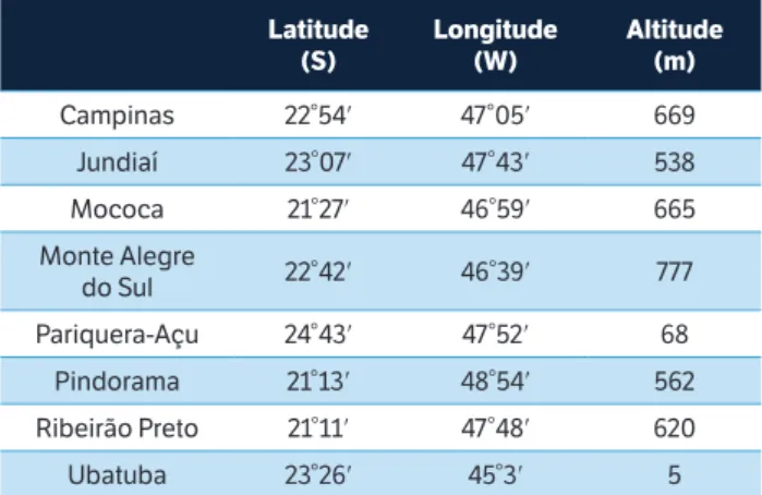
been evaluated in previous studies (Bardin-Camparotto et al. 2014; Blain et al. 2009). These weather stations also represent climatically dissimilar areas of the State, ranging from the coastal area (Ubatuba), where there is no distinctly dry season, to the northwestern region of the State (Ribeirão Preto), where there is a distinctly dry season during the winter months (see Appendices 1 and 2).

where: c₀ = 2.515517; c₁ = 0.802853; c₂ = 0.010328;

d₁= 1.432788; d₂= 0.189269; d₃ = 0.001308.

The SPI wet/drought categories are presented in Table 2. The frequently used Kolmogorov-Smirnov/Lilliefors test (KSL; Wilks 2011) was applied to assess the fit of the gamma distribution to the rainfall data obtained from all calibration periods. The Monte Carlo simulations required for calculating the critical values of this goodness-of-fit test were based on the procedure called “Non-uniform random number generation by inversion” (Wilks 2011; Blain 2014, among many others). Further information on this test, including its advantages over other goodness-of-fit tests, can be found in several studies such as Wilks (2011). The KSL

latitude (s) longitude (W) Altitude (m)

Campinas 22°54′ 47°05′ 669

Jundiaí 23°07′ 47°43′ 538

Mococa 21°27′ 46°59′ 665

Monte Alegre

do Sul 22°42′ 46°39′ 777

Pariquera-Açu 24°43′ 47°52′ 68

Pindorama 21°13′ 48°54′ 562

Ribeirão Preto 21°11′ 47°48′ 620

Ubatuba 23°26′ 45°3′ 5

table 1. Weather stations used to calculated the Standardized Precipitation Index (State of São Paulo, Brazil).

As described, the SPI can be computed for multiple time scales depending on the user’s interest, with typical values ranging from 1 to 12 months (Blain 2012b; Dutra et al. 2013). The time scales of 1, 3, 6, 9 and 12 months have been adopted because they are used in operational mode by the Drought Monitoring System of IAC/CIIAGRO. Although several pdfs may be used to calculate the SPI (Guttman 1999), the 2-parameter gamma distribution is the most used (Wu et al. 2005; Wu et al. 2007; Dutra et al. 2013; Stagge et al. 2015). Once a pdf is chosen (Equation 1), the cumulative probability [H(PRE)] of a given rainfall amount is obtained from Equations 2 and 3, in which the lower limit of the integral is zero because the precipitation distributions are zero-bounded) — q is the number of zeros in the data sample. As described by several studies, such as Wu et al. (2007), the final step of the SPI algorithm is based on the rational approach proposed by Abramowitz and Stegun (1965; Equations 4 and 5).

where: Г(α) is the gamma function; α and β are the distribution parameters; PRE is the rainfall amounts.

sPI values Drought category

≥ 2.00 Extremely wet

1.50 to 1.99 Very wet

1.00 to 1.49 Moderately wet

0.99 to −0.99 Near normal

−1.00 to −1.49 Moderately dry

−1.50 to −1.99 Severely dry

≤ −2.00 Extremely dry

table 2. Standardized Precipitation Index values and the associated drought categories.

SPI = Standardized Precipitation Index. Extracted from the Standardized Precipitation Index User Guide: WMO Nº1090. www.wamis.org/agm/pubs/ SPI/WMO_1090_EN.pdf (2) (3) (5) (1) (4) H(PRE) ≤ 0.5 0 for t d t d t d 1 t – SPI ₃ 3 2 2 1 < + + + = –

c₀ + c₁ + c₂t2

H(PRE) <1 0.5 for t d t d t d 1 t – SPI ₃ 3 2 2 1 < + + + = –

c₀ + c₁ + c₂t2

H(PRE) ≤ 0.5 0

for < (H(PRE))2

1

ln(

t =

H(PRE) <1 0.5

for < (H(PRE))2

1 ln( t =

H(PRE) = q + (1 – q)Gam(PRE) =

PRE

0

gam(PRE)d(PRE) Gam(PRE)

PREα–1 _{· e}–PRE/β

βα_Γ(α)

(4)

test was calculated at the 5% significance level by means of an r-code (R-software) adapted from Blain (2014; Appendix 3). As previously described, the SPI was designed as a spatially invariant drought index (Guttman 1999). In other words, a SPI series must be capable of meeting the normality assumption (Wu et al. 2007; Blain 2012a,b; Stagge et al. 2015). Therefore, we applied an algorithm proposed by Wu et al. (2007) to verify the normality assumption of the SPI series derived from the different calibration periods evaluated in this study. According to this algorithm, a SPI series is considered non-normal when the 2 following criteria are simultaneously met: (1) absolute value of the median greater than 0.05; (2) Shapiro-Wilk’s (SW) statistic test lower than 0.96 and p-values ≤ 0.10. For further information on the Shapiro-Wilk’s test, see Razali and Wah (2011).

The degree of correlation among the SPI values obtained from the different calibration periods was initially evaluated by means of the linear correlation analysis as suggested by Wu et al. (2005). However, it is well-known that the

magnitude of the r2_{coefficient is not consistently related}

to the degree to which SPI values, derived from different sample sizes, approach each other (Willmott 1982; Wu et al. 2005, among many others). This degree of accuracy (or agreement) was measured by the modified index of agreement

(d_mod; Willmott et al. 1985) and by the absolute mean error

(AME), which can be thought as a scalar measurement of the average difference between 2 datasets (Wilks 2011).

The d_mod is bounded by 0 and 1. A perfect fit between SPI

values obtained from the 30-year calibration period in respect to those derived from other calibration periods

(< 30 years) would lead to d_mod= 1. When applied to a given

data bunch, the d_mod will be lower or, at most, equal to the

original index of agreement (further information regarding the difference between the original index of agreement and its modified version can be found in Willmott et al. 1985). Quantitative estimates of both systematic and random errors were made according to Equations 6 and 7, respectively (Willmott 1982):

SPI value calculated from calibration periods smaller than

30 years;

P

ˆ

represents the predicted SPI values according

to the linear regression equation; MSE_s and MSE_r are,

respectively, the systematic and random components of the error.

Finally, as an operational assessment of the consistency of the SPI values derived from different calibration periods, all SPI monthly values observed during 2013 and 2014 have been compared in respect to their wet/drought categories (Table 2). This qualitative assessment is similar to those found in Wu et al. (2005). These 2 years (2013 and 2014) have been selected because, since 2013, the State of São Paulo has been subjected to an extreme/severe drought event (as shown in the next section).

resUlts AND DIscUssIoN

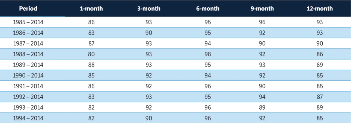
Before analyzing the results of the KSL test (Table 2), it has to be emphasized that several 3-parameter distributions, such as generalized normal distribution (Meschiatti and Blain 2015) and Pearson’s type III (Guttman 1999; Vicente-Serrano et al. 2012; Blain 2012b), have also been recommended to calculate the SPI because they are more flexible than the 2-parameter gamma. However, Stagge et al. (2015) remind that a 3-parameter distribution allows negative values. Naturally, when these functions are used in studies dealing with rainfall series, they must be truncated at zero. In addition, Stagge et al. (2015) are of the opinion that adding an extra parameter is an unnecessary complication given the relative small sample sizes (or calibration periods) that are frequently used to calculate the SPI. The results of the KSL test (Table 3) agree with these latter statements, given that the average acceptance rates of the gamma distribution were higher than 92% for all calibration periods and time scales.

The acceptance rates presented in Table 3 are also consistent with those found by Stagge et al. (2015), who, as previously described, recommended the use of gamma distribution to calculate the SPI throughout Europe. Therefore, we may state that the KSL test has provided evidences in favor of the use of gamma distribution to calculate the SPI in the State of São Paulo. However, in spite of the fact that this latter statement holds for all calibration periods evaluated in Table 3 (21 to 30 years), it has to be emphasized that the KSL is a relatively insensitive test because where: N is the sample size; O is the SPI value calculated

from the standard 30-year period (1985 – 2014); P is the (6)

(7) N

i = 1 MSE_s = N–1

Σ

(Pi – Oi) 2 ˆ

N

i = 1 MSE_r = N–1

Σ

(Pi – Pi) 2

(5)

both empirical and theoretical distributions converge to zero and/or one in their tails (Stagge et al. 2015; Kruel et al. 2015). This statement is consistent with the fact that the acceptance rates of the normality test (Table 4) are lower than those of the KSL test. This fact is also consistent with the results presented by Stagge et al. (2015) for Europe, where the rejection rates of the KSL test were, on average, 7% lower than those of the Shapiro-Wilk’s test.

The results presented in Table 4 indicate that, even for the 30-year period, the normally assumption is not always met. In other words, even those SPI series calculated from the continuous 30-year period recommended by McKee et al. (1993) and regarded by Stagge et al. (2015) as “the standard period for the SPI calculation” are not always capable of meeting the assumption of normality. This statement is particular true for the monthly time scale and may be

explained by the presence of zero values in the rainfall series (see Appendix 2) that leads the SPI to be a lower bounded index (Wu et al. 2007; Blain 2012a; Stagge et al. 2015). This statement is also the reason why Wu et al. (2007) recommended that the SPI user be cautious when using this drought index at short-time scales. By analyzing the results presented in Table 4, one is also able to verify that the rejection rates of the normality test observed in this study (which varied from 2 to 20%) are, in general, lower than those found by Stagge et al. (2015). According to these authors, in some regions of Denmark, France and Greece, the normality assumption of the SPI series (calculated from the gamma distribution) varied from 15 to 40%.

By considering the general goal of this study (i.e. the operational use of the SPI), the results presented in Table 4 do not indicate remarkable differences among the rejection/

Period 1-month 3-month 6-month 9-month 12-month

1985 – 2014 86 93 95 96 93

1986 – 2014 83 90 95 92 93

1987 – 2014 87 93 94 90 90

1988 – 2014 80 93 98 92 86

1989 – 2014 88 93 95 93 89

1990 – 2014 85 92 94 92 85

1991 – 2014 86 92 96 90 85

1992 – 2014 83 93 95 94 87

1993 – 2014 82 92 96 89 89

1994 – 2014 82 90 96 92 85

Period 1-month 3-month 6-month 9-month 12-month

1985 – 2014 95.2 94.0 91.7 90.5 92.9

1986 – 2014 92.9 92.9 94.0 94.0 92.9

1987 – 2014 95.2 91.7 96.4 96.4 96.4

1988 – 2014 96.4 94.0 92.9 96.4 94.0

1989 – 2014 95.2 96.4 95.2 97.6 96.4

1990 – 2014 96.4 97.6 96.4 95.2 96.4

1991 – 2014 97.6 96.4 96.4 96.4 97.6

1992 – 2014 97.6 98.8 98.8 96.4 97.6

1993 – 2014 92.9 90.5 94.0 94.0 90.5

1994 – 2014 94.0 95.2 94.0 96.4 96.4

table 4. Average acceptance rates (%) of the normally assumption of Standardized Precipitation Index series calculated at the following time scales: 1; 3; 6; 9 and 12 months. The acceptance rates have been obtained by applying a normality test, proposed by Wu et al. (2007), to 9 locations of the State of São Paulo, Brazil.

(6)

M.C. Meschiatt i and G.C. Blain

acceptance rates obtained from the diff erent calibration periods. For instance, the average acceptance rate of the monthly SPI series derived from the 30-year and 21-year periods are,

respectively, 86 and 82%. Th e great diff erence among the

acceptance rates is observed for the 12-month SPI series in which the acceptance rate varied from 93% (30 years) to 85%

(21 years). Th erefore, regarding the normality assumption, the

results presented in Table 4 indicated that the performance of the SPI series derived from the smallest calibration period (21 years, 1994 – 2014) was equivalent to the performance of the SPI series obtained from the 30-year period of 1985 – 2014

in 93% of the cases (at least). Th e results presented in Tables

3, 4 allowed us to quantify the correlation, the agreement and the consistency of SPI values obtained from the calibration periods ranging from 29 to 21 years in respect to the SPI values obtained from the standard 30-year period.

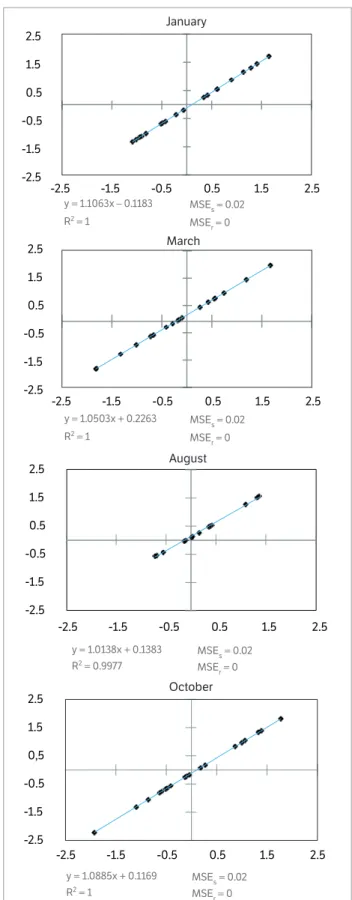
Th e linear correlation analysis indicated a lack of random

errors among the SPI values obtained from the 30-year period in respect to those obtained from other (smaller) lengths of records. As exemplifi ed in Figure 1, for the weather station of Campinas (monthly SPI values, considering the 30-year and 21-year calibration periods), the linear correlation analysis reveals that using calibration periods smaller than 30 years to

calculate the SPI leads to non-random error. Th is statement

is also supported by the MSE_r and MSE_s values presented in

Figure 1. As can be noted, only the systematic component of

the MSE is greater than zero. Th e results of all other regression

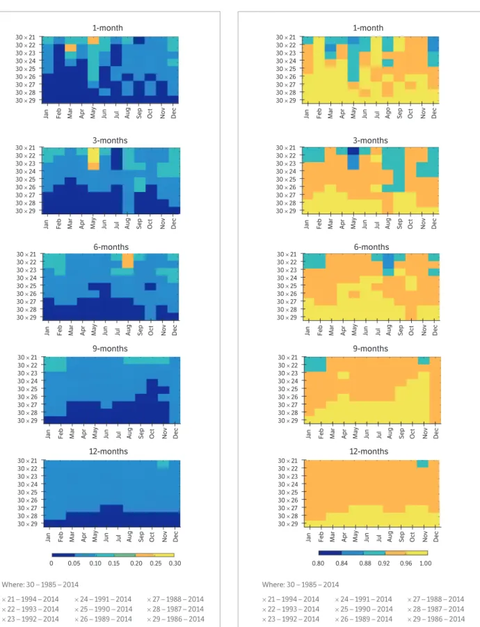
analyses were equivalent to those depicted in Figure 1. Similar to the results found by Wu et al. (2005), the AME values increased as the length of the calibration periods decreased (Figure 2). For instance, no AME > 0.1 was observed for calibration periods equal to or larger than 27 years. On the other hand, the highest AMEs are observed for the smallest calibration periods (22 and 21 years). For these periods, AME has reached values greater than 0.25. By considering that 0.5 is the numerical diff erence between a severe and an extreme drought event (Table 2), these latter AME values suggest that calibration periods starting aft er 1991 should not be used to derive SPI values in the State

of São Paulo. Th is latter inference is consistent with the

results depicted in Figure 3. By following Wu et al. (2005),

we may assume that values of d_mod equal to or greater than

0.90 describe a high (and acceptable) agreement between 2 SPI series derived from diff erent calibration periods. In

this view, no d_mod < 0.9 is observed for calibration periods

starting in 1991 (or earlier; Figure 3).

Figure 1. Linear regression analysis — Standardized Precipitation Index monthly values for 1985 – 2014 (x-axis) and Standardized Precipitation Index monthly values for 1994 – 2014 (y-axis). Campinas, State of São Paulo.

-2.5 -1.5 -0.5 0.5 1.5 2.5

-2.5 -1.5 -0.5 0,5 1.5 2.5

-0,5 0,5 1,5

-2.5 -1.5 -0.5 0.5 1.5 2.5

January

March

August

October

y = 1.1063x – 0.1183 R2_{= 1}

MSE_s = 0.02 MSE_r = 0

y = 1.0503x + 0.2263 R2_{= 1}

MSE_s = 0.02 MSE_r = 0

y = 1.0138x + 0.1383 R2_{= 0.9977}

MSE_s = 0.02 MSE_r = 0

y = 1.0885x + 0.1169 R2_{= 1}

(7)

Figure 2. Absolute mean error of Standardized Precipitation Index values derived from calibration periods ranging from 1994 – 2014 to 1986 – 2014 (21 to 29 years) in respect to Standardized Precipitation Index values derived from 1985 – 2014. State of São Paulo, Brazil.

Figure 3. Modified index of agreement (d_mod) of Standardized Precipitation Index values derived from calibration periods ranging from 1994 – 2014 to 1986 – 2014 (21 to 29 years) in respect to Standardized Precipitation Index values derived from 1985 – 2014. State of São Paulo, Brazil. 1-month

May

Apr

Mar

Feb

Jan Jun Jul Aug Sep Oct Nov Dec

30 × 29 30 × 28 30 × 27 30 × 26 30 × 25 30 × 24 30 × 23 30 × 22 30 × 21

3-months

May

Apr

Mar

Feb

30 × 29 30 × 28 30 × 27 30 × 26 30 × 25 30 × 24 30 × 23 30 × 22 30 × 21

6-months

May

Apr

Mar

Feb

30 × 29 30 × 28 30 × 27 30 × 26 30 × 25 30 × 24 30 × 23 30 × 22 30 × 21

9-months

May

Apr

Mar

Feb

30 × 29 30 × 28 30 × 27 30 × 26 30 × 25 30 × 24 30 × 23 30 × 22 30 × 21

12-months

May

Apr

Mar

Feb

30 × 29

0 0.05 0.10 0.15 0.20 0.25 0.30

Where: 30 – 1985 – 2014

× 21 – 1994 – 2014

× 22 – 1993 – 2014

× 23 – 1992 – 2014

× 24 – 1991 – 2014

× 25 – 1990 – 2014

× 26 – 1989 – 2014

× 27 – 1988 – 2014

× 28 – 1987 – 2014

× 29 – 1986 – 2014 30 × 28

30 × 27 30 × 26 30 × 25 30 × 24 30 × 23 30 × 22 30 × 21

1-month

May

Apr

Mar

Feb

Jan Jun Jul Ago Sep Oct Nov Dec

30 × 29 30 × 28 30 × 27 30 × 26

30 × 25

30 × 24 30 × 23

30 × 22

30 × 21

3-months

May

Apr

Mar

Feb

30 × 29

30 × 28

30 × 27 30 × 26

30 × 25

30 × 24 30 × 23

30 × 22

30 × 21

6-months

May

Apr

Mar

Feb

30 × 29 30 × 28 30 × 27 30 × 26

30 × 25

30 × 24 30 × 23

30 × 22

30 × 21

9-months

May

Apr

Mar

Feb

30 × 29

30 × 28 30 × 27 30 × 26 30 × 25

30 × 24

30 × 23 30 × 22

30 × 21

12-months

May

Apr

Mar

Feb

30 × 29

0.80 0.84 0.88 0.92 0.96 1.00

Where: 30 – 1985 – 2014

× 21 – 1994 – 2014 × 22 – 1993 – 2014 × 23 – 1992 – 2014

× 24 – 1991 – 2014 × 25 – 1990 – 2014 × 26 – 1989 – 2014

× 27 – 1988 – 2014 × 28 – 1987 – 2014 × 29 – 1986 – 2014

30 × 28

30 × 27 30 × 26

30 × 25

30 × 24 30 × 23

30 × 22

(8)

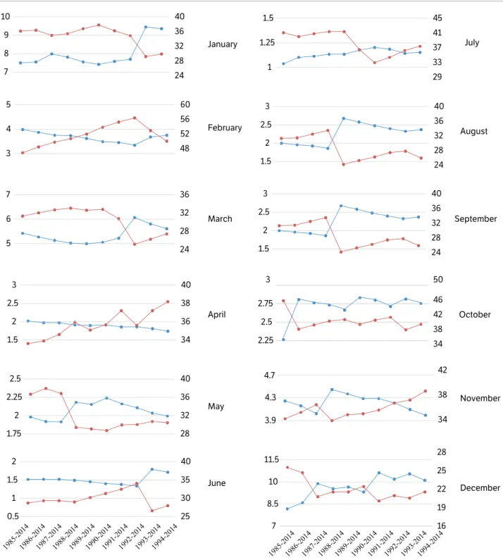
Considering that SPI values calculated from diff erent lengths of records are highly consistent and correlated only when the parameters of the gamma distributions are similar (Wu et al. 2005), the results of Figures 2, 3 (and the conclusion drawn from them) suggest a change in the rainfall distributions aft er 1991. Indeed, by evaluating the parameters

of this distributions calculated from the monthly series, we observed a remarkable change around 1992 – 1993, as exemplifi ed for the Weather Station of Campinas (Figure 4). Note that this last statement is particular true for the 8 of the 12 monthly series (January; February; March; April; May; June; July and November).

Figure 4. Shape(blue line) and scale (red line) of the gamma distribution calculated from diﬀ erent lengths of rainfall records (Campinas, São Paulo, Brazil).

20 24 28 32 36 40 6 7 8 9 10 January 40 48 52 56 60 2 3 4 5 February 20 24 28 32 36 4 5 6 7 March 34 36 38 40 1.5 2 2.5 3 April 25 29 33 37 41 45 0,75 1 1.25 1.5 July 20 24 28 32 36 40 1 1.5 2 2.5 3 August 24 28 32 36 40 1.5 2 2.5 3 September 34 38 42 46 50 2.25 2.5 2.75 3 October 28 32 36 40 1.75 2 2.25 2.5

May November

(9)

Case of study (operational mode)

Under the operational mode and regarding the question posed at the beginning of this study, the above-mentioned results allows us to infer that there will be no remarkable diff erence in the wet/dry SPI categories (Table 2) derived from calibration periods ranging from 1991 – 2014 to 1986 – 2014 in respect to those derived from 1985 – 2014 in the State of

São Paulo. Th e visual inspection of Figures 5 to 9 supports

this inference by describing virtually no diff erence in the

wet/dry categories characterized by SPI values derived from the smallest selected period (24 years; 1991 – 2014) in respect to the standard 30-year period of 1985 – 2014.

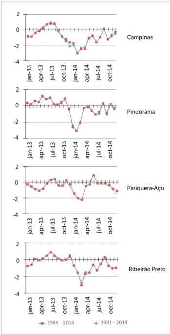
Regardless the calibration period, the results depicted in Figure 5 (monthly SPI) clearly indicate that 2014 has started

under severe to extreme dry conditions (SPI < −2.0). Th e

results depicted in Figure 5, along with those depicted in Figures 6 to 9, support the idea that the State of São Paulo has been subjected to a drought event expected to occur

once, on average, 100 – 700 years. Th e analysis of Figures

Figura 5. Standardized Precipitation Index derived from diﬀ erent calibration periods (time scale: 1-month) for 4 locations of the State of São Paulo.

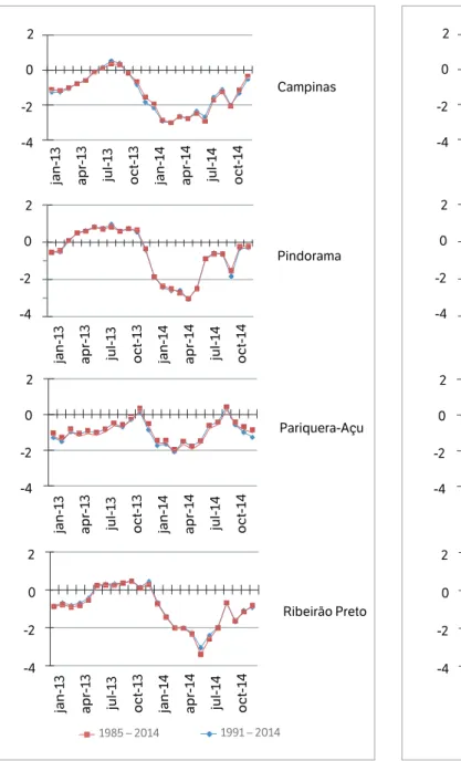
Figure 6. Standardized Precipitation Index derived from diﬀ erent calibration periods (time scale: 3-month) for 4 locations of the State of São Paulo.

-4 -2 0 2 -4 -2 0 2 -4 -2 0 2

-4 -2 0 2

jan-13 apr-13 jul-13 oct-13 jan-14 apr-14 jul-14 oct-14 jan-13 apr-13 jul-13 oct-13 jan-14 apr-14 jul-14 oct-14 jan-13 apr-13 jul-13 oct-13 jan-14 apr-14 jul-14 oct-14 jan-13 apr-13 jul-13 oct-13 jan-14 apr-14 jul-14 oct-14

1985 – 2014 1991 – 2014

Pariquera-Açu Pindorama Campinas

Ribeirão Preto

-4 -2 0

2 -4 -2 0 2 -4 -2 0 2

-4 -2 0 2

1985 – 2014 1991 – 2014

Ribeirão Preto

2

(10)

4 to 8 also emphasizes the importance of monitoring the rainfall defi cits at several time scales for detecting the onset of a drought as soon as possible (Hayes et al. 1999). In spite of the negative values depicted in Figure 5 (monthly SPI), it is not evident that a drought has been established. For instance, the monthly SPI value for January, 2014 (Pindorama, São Paulo) is −2.70 (1991 – 2014) or −3.20 (1985 – 2014). However, in March, 2014 this index has reached the near normal category by presenting values equal to 0.44 (calibration periods: 1991 – 2014) or 0.39

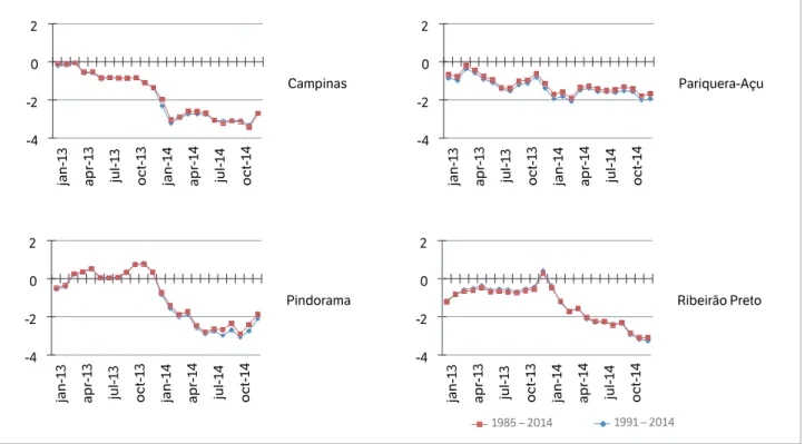
(calibration periods: 1985 – 2014; Figure 5). On the other hand, by analyzing this index at larger time scales (e.g. 6 to 12 months), one is able to verify that no positive SPI value has been recorded aft er January, 2014. Naturally, these negative SPI values observed at all time scales (Figures 4 to 8) indicate that a severe to extreme drought has been

established in the State of São Paulo since January, 2014. Th is

latter inference can be drawn from the SPI values derived from the 30-year period of 1985 – 2014 as well as from SPI values derived from the 24-year period of 1991 – 2014.

-4 -2 0 2 -4 -2 0 2

Pindorama Campinas

-4 -2 0 2

1985 – 2014 1991 – 2014

Pariquera-Açu

Ribeirão Preto

-4 -2 0

2 -4 -2 0 2 -4 -2 0 2

-4 -2 0 2

1985 – 2014 1991 – 2014

Ribeirão Preto

-1

(11)

-4 -2 0 2

jan-13 apr-13 jul-13 oct-13 jan-14 apr-14 jul-14 oct-14

1985 – 2014 1991 – 2014

Ribeirão Preto -4

-2 0 2

Pariquera-Açu

-4 -2 0 2

Pindorama -4

-2 0 2

Campinas

coNclUsIoN

There is high agreement among SPI values derived from the calibration period of 1985 – 2014 (30-year period) in respect to those SPI values derived from calibration periods ranging from 1991 – 2014 to 1986 – 2014. This conclusion allows using weather stations with rainfall

records starting in 1991 (or earlier) for the operational application of the Standardized Precipitation Index in the State of São Paulo, Brazil. This conclusion is based on evaluations of intrinsic features of the SPI. Therefore, the methods used in this study may be used to increase the regional availability of the Standardized Precipitation Index in any area of the globe.

Abramowitz, M. and Stegun, I. A. (1965). Handbook of mathematical

function. New York: Dover Publications.

Bardin-Camparott o, L., Blain, G. C., Pedro Júnior, M. J., Hernandes,

J. L. and Cia, P. (2014). Climate trends in a non-traditional high

quality wine producing region. Bragantia, 73, 327-334. htt p://dx.doi.

org/10.1590/1678-4499.0127.

Blain, G. C. (2012a). Revisiting the probabilistic definition of

drought: strengths, limitations and an agrometeorological

adaptation. Bragantia, 71, 132-141. http://dx.doi.org/10.1590/

S0006-87052012000100019.

Blain, G. C. (2012b). Monthly values of the standardized precipitation

index in the State of São Paulo, Brazil: trends and spectral features

reFereNces

under the normality assumption. Bragantia, 71, 460-470. htt p://

dx.doi.org/10.1590/S0006-87052012005000004.

Blain, G. C. (2014). Revisiting the critical values of the Lilliefors test:

towards the correct agrometeorological use of the

Kolmogorov-Smirnov framework. Bragantia, 73, 192-202. htt p://dx.doi.org/10.1590/

brag.2014.015.

Blain, G. C., Kayano, M. T., Camargo, M. B. P. and Lulu, J. (2009).

Variabilidade amostral das séries mensais de precipitação pluvial

em duas regiões do Brasil: Pelotas-RS e Campinas-SP. Revista

Brasileira de Meteorologia, 24, 1-11. htt p://dx.doi.org/10.1590/

(12)

Blain, G. C. and Meschiatti, M. C. (2015). Inadequacy of the gamma

distribution to calculate the Standardized Precipitation Index.

Revista Brasileira de Engenharia Agrícola e Ambiental, 19, 1129-1135.

http://dx.doi.org/10.1590/1807-1929/agriambi.v19n12p1129-1135.

Dutra, E., Di Giuseppe, F., Wetterhall, F. and Pappenberger, F.

(2013). Seasonal forecasts of droughts in African basins using

the Standardized Precipitation Index. Hydrology and Earth System

Sciences, 17, 2359-2373. http://dx.doi.org/10.5194/hess-17-2359-2013.

Guttman, N. B. (1999). Accepting the “Standardized Precipitation

Index”: a calculation algorithm. Journal of the American

Water Resources Association, 35, 311-322. http://dx.doi.

org/10.1111/j.1752-1688.1999.tb03592.x.

Hayes, M. J., Svoboda, M. D., Wall, N. and Widhalm, M. (2011).

The Lincoln Declaration on Drought Indices — universal

meteorological drought index recommended. Bulletin of the

American Meteorological Society, 92, 485-488. http://dx.doi.

org/10.1175/2010BAMS3103.1.

Hayes, M. J., Svoboda, M. D., Wilhite, D. A. and Vanyarkho, O. V. (1999).

Monitoring the 1996 drought using the Standardized Precipitation

Index. Bulletin of the American Meteorological Society, 80,

429-438. http://dx.doi.org/10.1175/1520-0477(1999)080<0429:MTDU

TS>2.0.CO;2.

Kruel, I. B., Meschiatti, M. C., Blain, G. C. and Avila, A. M. H. (2015).

Climate trends in a locality of southern Brazil. Engenharia Agrícola,

35, 769-777. http://dx.doi.org/10.1590/1809-4430-Eng.Agric.

v35n4p769-777/2015.

McKee, T. B., Doesken, N. J. and Kleist, J. (1993). The relationship of

drought frequency and duration to the time scales. In Proceedings

of the 8th_{Conference on Applied Climatology; Anaheim, USA.}

Razali, N. M. and Wah, Y. B. (2011). Power comparisons of

Shapiro-Wilk, Kolmogorov-Smirnov, Lilliefors and Anderson-Darling tests.

Journal of Statistical Modeling and Analytics, 2, 21-33.

Stagge, J. H., Tallaksen, L. M., Gudmundsson, L., van Loon, A. F. and

Stahl, K. (2015). Candidate distributions for climatological drought

indices (SPI and SPEI). International Journal of Climatology. http://

dx.doi.org/10.1002/joc.4267.

Vicente-Serrano, S. M., Beguería, S., Lorenzo-Lacruz, J., Camarero, J.

J., López-Moreno, J. I., Azorin-Molina, C., Revuelto, J., Morán-Tejeda,

E. and Sanchez-Lorenzo, A. (2012). Performance of drought indices

for ecological, agricultural, and hydrological applications. Earth

Interactions, 16, 1-27. http://dx.doi.org/10.1175/2012EI000434.1.

Wilks, D. S. (2011). Statistical methods in the atmospheric sciences.

San Diego: Academic Press.

Willmott, C. J. (1982). Some comments on the evaluation of model

performance. Bulletin of the American Meteorological Society, 63,

1309-1313. http://dx.doi.org/10.1175/1520-0477(1982)063<1309:SCO

TEO>2.0.CO;2.

Willmott, C. J., Ackleson, S. G., Davis, R. E., Feddema, J. J., Klink, K.

M., Legates, D. R., O’Donnell, J. and Rowe, C. M. (1985). Statistics for

the evaluation and comparison of models. Journal of Geophysical

Research: Oceans, 90, 8995-9005. http://dx.doi.org/10.1029/

JC090iC05p08995.

Wu, H., Hayes, M. J., Wilhite, D. A. and Svoboda, M. D. (2005). The

effect of the length of record on the Standardized Precipitation

Index calculation. International Journal of Climatology, 25,

505-520. http://dx.doi.org/10.1002/joc.1142.

Wu, H., Svoboda, M. D., Hayes, M. J., Wilhite, D. A. and Wen, F.

(2007). Appropriate application of the Standardized Precipitation

Index in arid locations and dry seasons. International Journal of

(13)

month campinas Jundiaí mococa monte Alegre do sul

shape scale shape scale shape scale shape scale

Jan 7.5 36.1 4.7 59.8 5.9 49.9 4.6 61.3

Feb 4.0 46.9 7.8 23.3 3.9 50.1 4.1 47.8

Mar 5.4 31.4 3.6 46.6 5.0 33.3 6.4 29.3

Apr 2.0 34.5 2.7 26.8 1.6 55.7 2.8 31.8

May 2.0 36.6 2.0 38.5 1.9 36.5 1.9 39.1

Jun 1.3 32.8 1.2 41.7 0.9 33.3 1.1 43.7

Jul 1.0 41.1 1.0 54.7 1.1 22.5 1.1 41.4

Aug 1.2 26.9 0.9 38.6 0.9 34.9 0.9 40.0

Sep 2.0 31.3 1.5 48.3 2.0 32.4 2.9 27.4

Oct 2.3 45.8 2.9 41.0 3.1 42.6 2.5 56.1

Nov 4.2 34.0 4.6 34.6 7.5 22.5 5.8 27.8

Dec 8.2 25.6 5.3 38.8 10.1 25.8 9.1 24.8

month Pariquera-Açu Pindorama ribeirão Preto Ubatuba

shape scale shape scale shape scale shape scale

Jan 4.9 54.8 5.9 47.0 6.0 46.2 6.5 49.1

Feb 5.7 41.0 4.0 52.3 3.3 66.5 2.7 108.6

Mar 6.9 31.8 4.3 36.9 5.9 28.3 3.7 85.9

Apr 4.8 21.0 3.5 23.5 1.4 52.4 2.9 80.0

May 2.6 34.7 1.6 39.7 1.2 52.3 4.5 29.5

Jun 2.0 37.4 0.6 49.2 0.6 46.7 1.9 43.5

Jul 1.8 49.8 0.9 28.8 0.9 26.8 2.3 45.1

Aug 1.6 31.4 0.8 47.1 0.6 53.6 2.7 27.6

Sep 2.1 51.6 1.2 52.0 1.0 56.4 6.5 27.7

Oct 5.6 21.1 2.6 38.4 3.7 27.1 5.0 47.3

Nov 3.6 29.8 4.7 29.0 6.0 30.2 6.1 40.3

Dec 7.3 23.9 6.7 31.1 7.2 35.4 5.2 56.8

(14)

campinas cordeirópolis mococa monte Alegre do sul

Pre % Pre = 0 Pre % Pre = 0 Pre % Pre = 0 Pre % Pre = 0

Jan 261.8 0.0 251.3 0.0 279.1 0.0 267.5 0.0

Feb 180.9 0.0 180.0 0.0 193.7 0.0 195.8 0.0

Mar 157.1 0.0 162.7 0.0 157.2 0.0 167.9 0.0

Apr 73.8 0.0 78.7 0.0 84.8 0.0 87.7 0.0

May 70.9 0.0 61.7 0.0 64.1 0.0 70.5 0.0

Jun 49.3 8.9 48.2 8.9 34.2 15.6 52.3 6.7

Jul 39.4 8.9 35.1 6.7 26.2 11.1 41.3 8.9

Aug 30.8 17.8 28.9 26.7 24.6 26.7 34.5 15.6

Sep 67.7 2.2 67.5 4.4 70.6 2.2 76.2 2.2

Oct 112.6 0.0 112.5 0.0 125.2 0.0 129.8 0.0

Nov 144.4 0.0 155.6 0.0 181.1 0.0 165.5 0.0

Dec 212.6 0.0 218.6 0.0 269.3 0.0 233.8 0.0

Pariquera-Açu Pindorama ribeirão Preto Ubatuba

Pre % Pre = 0 Pre % Pre = 0 Pre % Pre = 0 Pre % Pre = 0

Jan 238.3 0.0 269.1 0.0 275.3 0.0 330.6 0.0

Feb 206.0 0.0 197.9 0.0 214.5 0.0 259.8 0.0

Mar 211.2 0.0 161.0 0.0 160.8 0.0 265.9 0.0

Apr 99.0 0.0 81.1 4.4 84.2 0.0 203.1 0.0

May 91.9 0.0 61.9 0.0 61.6 0.0 112.3 0.0

Jun 72.3 0.0 35.5 15.6 35.4 17.8 79.8 0.0

Jul 66.6 2.2 28.6 17.8 27.5 13.3 82.6 2.2

Aug 50.8 4.4 26.2 24.4 23.5 31.1 72.8 4.4

Sep 98.4 0.0 63.2 4.4 60.6 0.0 165.8 0.0

Oct 108.7 0.0 106.1 0.0 117.2 0.0 201.0 0.0

Nov 120.5 0.0 142.4 0.0 178.0 0.0 237.3 0.0

Dec 174.0 0.0 223.9 0.0 269.8 0.0 283.5 0.0

Appendix 2. Average rainfall amounts and frequency of zero rainfall values. State of São Paulo (1985 – 2014).

(15)

################

# datamatrix is a matrix in which each column corresponds to each month #As can be observed in this code all years must present 12 rainfall amounts datamatrix= as.matrix(read.table(“datamatrix.txt”, head=T))

shape=matrix(NA,12,1) scale=matrix(NA,12,1) Dmax=matrix(NA,12,1) NKSLcrit5=matrix(NA,12,1) NKSLcrit10=matrix(NA,12,1) pvalue=matrix(NA,12,1) for (month in 1:12){ data=datamatrix[,month] data1=data> 0

datap=data[data1] # the 2-parameter gamma is undefined for x < 0 n=length(data)

np=length(datap) nz=n-np

probzero=(n-nz)/n Ns=50000

probacum=matrix(NA,np,1) lilliefors=matrix(NA,Ns,1) probpar= matrix(NA,np,1)

A=log(mean(datap))-((sum(log(datap)))/np) shape[month,1]=(1/(4*A))*(1+sqrt(1+(4*A/3))) scale[month,1]=mean(datap)/shape[month,1] pos=matrix(1:np, np, 1)/np

probacum[,1]= (pgamma(sort(datap), shape[month,1], 1/scale[month,1], lower.tail = TRUE, log.p = FALSE)) Dmax[month,1]=max(abs(pos- probacum))

########Lilliefors x=matrix(NA,np,1) lilliefors=matrix(NA,Ns,1) probpar=matrix(NA,np,1) poss=matrix(1: np, np, 1)/np for (i in 1:Ns){

x[,1]=rgamma(np,shape[month,1],1/scale[month,1]) As=log(mean(x))-((sum(log(x)))/np)

alfals=(1/(4*As))*(1+sqrt(1+(4*As/3))) betals=mean(x)/alfals

probpar[,1]=pgamma(sort(x), alfals, 1/betals, lower.tail = TRUE, log.p = FALSE) Dmaxs=max(abs(poss- probpar))

lilliefors[i,1]=Dmaxs}

NKSLcrit5[month,1]=quantile(lilliefors, probs=0.95) NKSLcrit10[month,1]=quantile(lilliefors, probs=0.90) m=lilliefors>Dmax[month,1]

pvalue[month,1]=(length(lilliefors[m]))/Ns}

Goodness=c(“shape”, shape, “scale”, scale, “Dmax”, Dmax, “NKSLcrit5%”, NKSLcrit5, “NKSLcrit10%”, NKSLcrit10, “p-value”, pvalue) write.csv(Goodness, “GoodnessGamma.csv”)

##############