Does contagion really matter: real role of Greece in the sovereign bond crisis

(1)

DOES CONTAGION REALLY MATTER

Real role of Greece in the Sovereign Bond Crisis

Zongyuan Li

Dissertation submitted as partial requirement for the conferral of

Master in Finance

Supervisor:

Prof. António Manuel Rodrigues Guerra Barbosa, ISCTE Business School, Department of Finance

(2)

I Resumo: Este trabalho tem por objectivo identificar a eventual existência e a magnitude da

influência do mercado de dívida pública Grega nos mercados de dívida pública de outros países da União Económica e Monetária (UEM) durante o período da Crise das Dívidas Soberanas. Em primeiro lugar, foram analisados os coeficientes de correlação dínamica entre as variações dos riscos de cauda das obrigações a 5 anos Gregas e as obrigações a 5 anos de outros três países da UEM (Itália, Espanha e França) usando o modelo Dynamic Conditional Correlation (DCC). Os resultados indicam a existência de um efeito de contágio nas correlações, embora as correlações tendam a diminuir, quando o risco de cauda das obrigações Gregas aumenta. Em segundo lugar, tentou-se distinguir entre interdependência e contágio entre as obrigações Gregas e as obrigações de outros países da UEM. Os resultados apontam para a existência de contágio nas obrigações de todos os países da UEM no dia seguinte à ocorrência de um evento de crédito nas obrigações Gregas, mesmo após a exclusão de efeitos de interdependência entre os mercados. No entanto, este efeito de contágio tendeu a desaparecer durante o período da Crisa das Dívidas Soberanas, especialmente para os países mais estáveis (Áustria, Bélgica, França, Alemanha e Holanda).

(3)

II Abstract: The main purpose of this article is to identify the existence and extent of the influences

of the Greek sovereign bond market on other European Economic and Monetary Union (EMU) countries' sovereign bond markets during the Sovereign Bond Crisis. First, we analyze the dynamic correlation coefficients between the percentage changes of the tail risks of Greek 5 year sovereign bonds and the 5 year sovereign bonds of other three EMU countries (Italy, Spain and France) using the Dynamic Conditional Correlation (DCC) model. We find volatility spillover exists between Greece and other EMU countries, but the overall correlation coefficients decrease, with the increasing tail risks of Greek sovereign bonds. Second, we distinguish between interdependence and shift contagion, and find that there were statistically significant shift contagions in all of the EMU sovereign bonds on the day after the Greek credit events, even after excluding the effects of interdependence, between 2006 and 2011. However, we also find that the statistically significant shift contagions in the short term disappeared during the Sovereign Bond Crisis, especially in stable countries (Austria, Belgium, France, Germany and Netherlands).

Key words: Value at Risk, Sovereign bond Crisis, contagion, volatility spillover JEL Classification: C52, F30, G15

(4)

III

The European Sovereign Bond Crisis in 2010 was, to some degree, triggered by the Subprime Crisis started in late 2007. And the Subprime Crisis forced regulators, investors, and rating agencies to reevaluate the risk of the traditional “risk-free” and “low risk” financial securities, among the sovereign bonds of the European Economic and Monetary Union countries.

Most European countries were seriously affected by the Sovereign Bond Crisis, in particular Greece, Ireland, Italy, Portugal and Spain (GIIPS). These countries, with huge stocks of sovereign debt, rampant budget deficits and stagnated economies, began, one by one, to lose the trust of investors in the bond market once the latter realized that not all Euro-denominated bonds were alike. This meant that GIIPS countries faced major difficulties to secure new funds in the bond market and soaring yield rates. Eventually, some of these countries lost the ability to issue new debt at sustainable interest rates, forcing them to secure their financing needs through a rescue plan by the European Union (EU), the European Central Bank (ECB) and International Monetary Fund (IMF), jointly known as the “Troika”. In return, the rescued countries had to cut down the government expenditure and make structure reforms in order to create the conditions to return to a path of economic growth, thus reconstructing the confidence of financial markets. Not surprisingly, the difficulties spilled to the private sector, which also faced major difficulties in seeking funds from the banking sector and from the global financial market, and soaring interest rates. Furthermore, the big cuts in the government expenditure in the rescued countries and everywhere else in the EU, resulted in unemployment and recession, which put even more pressure on the government budgets, fueling a vicious circle of austerity, unemployment and recession that eventually spread across almost all countries in the EU.

This transmission of financial difficulties across regions is a typical symptom in recent large financial crisis. It was the case in the US stock market crash of 1987 (Black Monday), the speculative attacks on currencies in European Exchange Rate Mechanism between 1992 and 1993, the Asian financial crisis of 1997, the dot-com Bubble of 2001, the Subprime Crisis between 2007 and 2008 and the European Sovereign Bond Crisis of 2010.

When it comes to EMU sovereign bond market, the existence of risk contagion is well documented in the literature. Even before the Subprime and Sovereign Bond Crisis, Clare and

(6)

2

Lekkos (2000) and Skintzi and Refenes (2006) showed the evidence of volatility spillover among the European sovereign bonds.

Following the Sovereign Bond Crisis, this topic gathers renewed interest. Missio and Watzaka (2011), Contancio (2012), Mink and Haan (2012), Kalbaska and Gatkowski (2012), Audige (2013), Buchholz and Tonzer (2013), Gunduz and Kayay (2013), and Elkhaldi, Chebbi and Naoui (2013) all tried to identify the contagion of the Sovereign Bond Crisis from different perspectives and to point out the root cause for the contagion.

Missio and Watzaka (2011) found that there is a positive correlation between Greek sovereign Credit default swaps (CDS) spreads (the differences between Greek sovereign CDSs and German sovereign CDSs) and those of the rest European countries’, Kalbaska and Gatkowski (2012) revealed that there is a significant effect from the CDS spreads of debt of GIIPS to the CDS spreads of France, Germany and the UK between 2005 and 2010. Audige (2013) highlighted the contagion effects from Greece to Ireland and Portugal in 2010.

Most of the previous articles focus on CDS, since, in theory, CDS should reflect the market expectation of the default risk. However, CDS is not the best choice to objectively estimate the tail risks. Before 2008, all of the CDS transactions had to be done in the over-the-counter (OTC) market, and dealers did not need to publish market information. Only after November of 2008, because of the intense pressure by regulators, did the Depository Trust & Cleaning Corporation, which accounted for around 90% of the CDS market, start to release their CDS trades data on a weekly basis. In contrast, investors could easily access to the daily date of interest rates of sovereign bond market. All in all, the CDS market was neither transparent nor standardized before the Subprime Crisis. But more worryingly, it is questionable whether the CDS contracts were fairly priced, as the American International Group (AIG) episode demonstrated. AIG, the biggest CDS issuer during the Subprime Crisis, would go bankrupt due to the abrupt eruption of liquidity crisis caused by a sudden increase of collateral requirement of their CDS positions, if it could not receive the $182.3 billion bailout from the Treasury and the Federal Reserve Bank of New York.

In contrast, Value at Risk (VaR) is the generally accepted method to measure market risks, especially for financial institutions. It is the only acceptable internal market risk valuation model in BASEL III, and it even comes to be a worldwide standard model to quantify the market risk in

(7)

3

financial institutes1. For example, the EU had already applied the Capital Requirements Directive IV package to implement BASEL III agreement on January 1st, 2014, and the EU will also add some new provisions between 2014 and 2019. In the US, the Federal Reserve announced in 2011 that it would implement BASEL III rules.

Besides, VaR is also a widely used measure when analyzing the risk contagion and co-movements of systematic risks. For example, Reboredo and Ugolini (2014) tested the difference between co-movements of the systematic risks of European sovereign bonds before and after the Sovereign Bond Crisis by a CoVaR model; Polanski and Stoja (2014) analyzed the co-dependence of extreme events in Foreign Exchange markets by a Multidimensional Value at Risk model. Also, VaR is a popular measure to identify the credit events in previous articles. Nevertheless, no one, to the best of our knowledge, has analyzed the relation between the VaR of different sovereign bonds, thus we would like to fill in this blank.

In this paper, we estimate the market risk of each European sovereign bond market with VaR_𝑗,1,99%, which is the loss that security j will not excess within 1 day, at 99% confidence level.2 Since VaR is the basis of the whole analysis, our first step is to review the prevailing VaR models and find the most appropriate model to estimate VaR of EMU sovereign bonds. In section 3, we put several VaR models through a battery of tests and choose the most appropriate model to estimate the VaR of the EMU sovereign bonds with a punishment scorecard based on those tests.

After completing the estimations of the VaR of each sovereign bond, we use a Dynamic Conditional Correlation (DCC) model to analyze daily dynamic correlation coefficients between the percentage changes of VaR of Greek sovereign bonds and other sovereign bonds. The DCC model was first introduced by Engle (2002) as a simplified extension of traditional multivariate GARCH model, and then became the main methodology to identify risk spillover effects among

1_{Relation between Value at Risk and the Capital Requirement in BASEL III}

ct= max{VaRt−1,10,99%; mc× VaRavg} + max{sVaRt−1,10,99%; ms× sVaRavg}

where ct is the capital requirement at time t; VaRt−1,10,99% is the Value at Risk at time t-1, at the confidence level

99%, and period 10 days. VaRavg is the mean of last 60 days VaR at the confidence level 99% and period 10 days;

sVaRavg is the stressed Value at Risk at time t-1, at the confidence level 99%, and period 10 days. sVaRavg is the

mean of last 60 stressed VaR at the confidence level 99% and period 10 days; mc and ms are the multiplication

factors decided by supervisory authorities basing on the quality of VaR system, with a minimal value 3.

2_{Even though there is not a general scaling rule for all kinds of distributions. The scaling rule in BASEL III is}

(8)

4

countries. For instance, the DCC model was used by Missio and Watzaka (2011), and Elkhaldi,

Chebbi and Naoui (2013) to analyze the pattern of risk spillover effects between EMU countries during the Sovereign Bond Crisis.

In section 4, we apply the DCC model to estimate daily correlation coefficients and test how the VaR of Greek sovereign bonds influence the correlation coefficients between the percentage changes in the VaR of Greece and other countries (France, Italy, and Spain). We find, in general, that the correlation coefficients between percentage changes in the VaR of Greek and another countries’ sovereign bond tend to decrease, when the VaR of Greek sovereign bonds increase. And most of those decreases are statistically significant even though there are sporadic reversals.

Contagion, however, is commonly defined as an increment in cross-market linkages after a credit event in one country. But analysis based on the DCC model cannot test whether contagion exists after Greek credit events. Besides, the DCC model cannot help us distinguish “true” contagion from interdependence during crises. Kaminsky and Reinhart (2000) conceptually distinguished international financial crisis transmission through fundamentals-based channels and “true” contagion. After that, Forbes and Rigobon (2001, 2002) drew a distinction between contagion and interdependence and found that the evidence of contagion during 1987 U.S. stock market crash, 1994 Mexican Peso Devaluation, 1997 Asian Financial Crisis disappeared after adjusting heteroscedasticity bias.

As mentioned above, we need to identify and test the existence of “real” contagions in other EMU countries, following a credit event in Greek sovereign bonds. Hence, in Section 5, we regress the percentage changes of VaR of other EMU countries on global financial factors, country specific factors and also credit events of Greek sovereign bond market.

As Sy (2004) suggested, to be more comprehensive, credit events should be defined as distressed debt events rather than just defaults, since sovereign bonds can avoid default by bilateral or multilateral support. In this paper, we consider credit events as the extreme events in the lower tail of the sovereign bond’s profit and loss distribution, measured by VaR_j,99%.

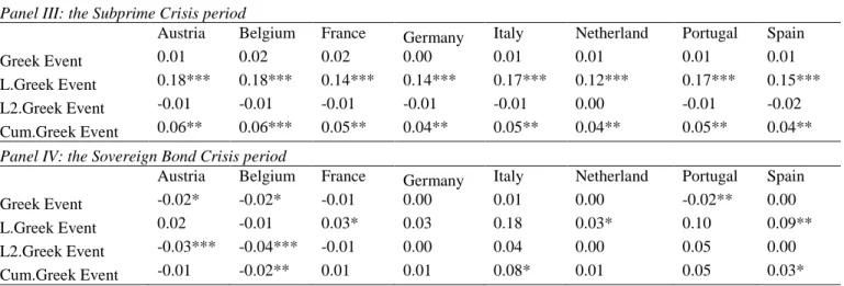
Since global factors capture the interdependence caused by global financial market and country-specific factors capture the influences of local substitutive markets, the coefficients of the Greek credit events indicators should reflect the extent of the shift contagions in other EMU sovereign

(9)

5

bonds, given the condition that there is a Greek credit event. In the end, we find that “real” contagions exist in all of other EMU countries’ (Austrian, Belgian, French, German, Italian, Dutch, Portuguese and Spanish) sovereign bonds before the Sovereign Bond Crisis. But the shift contagion disappears in the short term, especially in the stable countries (Austria, Belgium, France, Germany and Netherlands) during the Sovereign Bond Crisis.

The rest of this thesis proceeds as follows, Section 2 shows that the correlation coefficients between base point changes in sovereign bond yields are different from the correlation coefficients between the VaR of sovereign bonds, thus we cannot use the first correlation coefficients measure as a proxy to the second correlation coefficients measure. Subsequently, in Section 3, we select the most appropriate VaR model for EMU sovereign bond market using a punishment scorecard based on a battery of back tests. Section 4 presents the analysis of the pattern of dynamic correlation coefficients between Greece and some other countries. Section 5 distinguishes between “true" contagion and interdependence. And Section 6 summarizes the evidence and inferences made throughout the thesis.

2. Can the correlation between base point changes in bond yields represent the correlation between percentage changes of VaR of bonds?

If the dynamic correlation coefficients between base point changes in bond yields of every two EMU sovereign bonds can efficiently represent the daily correlation coefficients between percentage changes of VaR of those two EMU sovereign bonds, then there is no benefit in focusing our analysis on the VaR. In fact, under such circumstances, using the VaR would just introduce a second layer of estimation risk. Since the goal of section 4 is to identify and analyze the pattern of the correlation coefficients between the tail risks of Greek sovereign bonds and other EMU sovereign bonds, we want to test whether the correlation coefficients between base point changes in bond yields could efficiently represent the correlation coefficients between the percentage changes of bonds’ VaR.

As we have discussed in the introduction, CDS is not an appropriate proxy to represent the tail risks of sovereign bond market, because of the lack of transparency and regulation in the CDS

(10)

6

market. Therefore, we use the Value at Risk of 5 year Generic Government Rates as a better proxy for the tail risks of EMU 5 year sovereign bond market.

To estimate the tail risks of EMU sovereign bond market, we use the prevailing VaR model, EWMA volatility adjusted historical simulation, proposed by Hull and White (1998), the VaR model that works best in EMU sovereign bond market according to our discussion in section 3 .3

We generate two series of correlation estimates between sovereign bonds, one for base point changes in bond yields, the other for the percentage changes of bonds’ VaR, using a rolling window of 10, 20 or 30 days.

To examine whether there are significant differences between those two correlation coefficients measures, we calculate the daily difference, d_{𝑖𝑗,𝑡}, as equation 1 shows.

𝐝_{𝐢𝐣,𝐭}= 𝛒̂_{𝐢𝐣,𝐭,𝐛𝐩}− 𝛒̂_{𝐢𝐣,𝐭,𝐕𝐚𝐑%} (1)

where ρ̂_ij,t,bp is the correlation coefficient between country i’s and country j’s base point changes in bond yield at time t; and ρ̂_ij,t,VaR, is the correlation coefficients between the percentage changes of the VaR of country i’s and country j’s bonds at time t.

Figure 1: Differences between two different correlation measures

The correlation coefficients between base point changes in bond yields and percentage changes of the VaR of German and Italian sovereign bonds are estimated using a rolling window of 10, 20, and 30 days, respectively, (ρ̂Germany,Italy,t,bp or ρ̂Germany,Italy,t,VaR, t = 2006 Jan 2⁄ ⁄ to 2013 Dec 31⁄ ⁄ ) as in the graphs V(A) and V(B).4 Since

we estimate the daily correlation coefficients by the rolling window method, we do not have valid correlation coefficients at beginning 10, 20 or 30 days, respectively.

Graphs I, II, and III, depict the daily differences between the correlation coefficients between base point changes of the German and Italian sovereign bond yields and the correlation coefficients between the percentage changes of the VaR of those two markets with window size 10 days, 20 days and 30 days, respectively. dGermany,Italy,t= ρ̂Germany,Italy,t,bp− ρ̂Germay,Italy,t,VaR.

3_{We will introduce the details of this method in section 3. And the brief idea of this method is to adjust the}

historical base point changes by current variance and historical variance, and estimate daily VaR by last 500 volatility adjusted base point changes and the risk exposure (present value of 1 base point change). bpj,t∗ = σj,T

bpj,t

σj,t

Where bp𝑗,𝑡 is the historical base point changes of security j at time t; σ𝑗,𝑡 is the historical daily standard deviation

of base point changes of security j at time t; σ𝑗,𝑇 is the daily standard deviation of base point changes of security j

at target time T; bpj,t∗ is the adjusted historical base point changes of security j at time t;

Daily variance is estimated by EWMA method, σj,t2 = λσj,t−12 + (1 − λ) bpj,t−12 , where λ = 0.94

4_{The window size of 5 year Generic Government Rates are between 2003 Jan 2}nd_{and 2013 Dec 31}st_{, but we have}

(11)

7 Graph IV depicts the Value at Risk of German and Italian 5 year sovereign bonds. VaR is estimated by EWMA volatility adjusted historical simulation proposed by Hull and White, where λ = 0.94

Graphs V (A) and V (B) depict the correlation coefficients between base point changes in bond yields and the percentage changes of the VaR of German and Italian 5 year sovereign bonds, respectively.

Graph I: the differences between correlation coefficient measures (window size equals 10)

Graph II: the differences between correlation coefficient measures (window size equals 20)

Graph III: the differences between correlation coefficient measures (window size equals 30)

Graph IV: Value at Risk of German and Italian 5 year

sovereign bonds

Graph V(A): the correlation coefficients between base point changes of German and Italian Sovereign bond yields

Graph V (B): the correlation coefficients between percentage changes of VaR of German and Italian

sovereign bonds -2.5 -2 -1.5 -1 -0.5 0 0.5 1 1.5 -2 -1.5 -1 -0.5 0 0.5 1 -2 -1.5 -1 -0.5 0 0.5 1 0 2000 4000 6000 8000 10000 12000 14000

VaR Germany VaR Italy

-1.5 -1 -0.5 0 0.5 1 1.5

10 days 20 days 30 days

-1 -0.5 0 0.5 1 1.5

(12)

8

As we can see from Graph I to III of Figure 1, before 2008, two correlation coefficient series track each other quite well. The differences between those two correlation coefficient series seldom deviate from 0. We can also reach a same conclusion by observing Graph V (A) and V (B) of Figure 1, where we can see that the correlation coefficients are always close to 1. Meanwhile, the VaR of German and Italian sovereign bonds are low and stable throughout that period of time, as we can see from Graph IV of figure 1.

Between 2008 and 2009, the differences become more volatile as we can observe from Graph I to III of Figure 1. According to the Graph V (A) and V (B) of Figure 1, the volatility of the correlation coefficients between the percentage changes of the VaR is larger than the volatility of the correlation coefficients between base point changes in bond yields. During those two years, the VaR of German and Italian sovereign bonds have nearly doubled, but those two correlation coefficients series still track each other to some degree, as Graph IV of Figure 1 shows.

Nevertheless, after 2010, when the VaR of Italian sovereign bond is soaring, the differences between those two correlation coefficients measures become very volatile.

All in all, the differences between those two correlation coefficients measures are significant, if the tail risks of either or both of the sovereign bonds are high.

The reason why we could observe such situation could be that VaR will accumulate the effects of recent base point changes in bond yields. Thus, those two correlation coefficients series would be different from each other, especially during the financial turmoil.

We could also draw similar conclusions when analyzing the correlation coefficients between German and Belgian 5 year sovereign bonds, German and Austrian 5 year sovereign bonds, German and Greek 5 year sovereign bonds, and Greek and Italian 5 year sovereign bonds. Thus, it is a general case for the EMU sovereign bond market rather than a specific case for some specific EMU countries.

To complement the evidence from Figure 1, we can also verify whether those two correlation coefficients measures are statistically different from each other using paired t tests in the overall sample period and each subsample period.

(13)

9

The null hypotheses of the paired t tests are that the correlation coefficients between base point changes are equal to the correlation coefficients between percentage changes of VaR, ρ̂_ij,t,bp− ρ̂_ij,t,VaR= 0.

With a single exception between Greek and German sovereign bonds between 2006 and 2013 with the rolling window 10 days, we always reject the null hypothesis at 99% confidence level as Table 1 shows.

Table 1: Paired t test of two correlation coefficients measures

We divide the overall sample period into three subsample, 2006 Jan. - 2007 Dec., 2008 Jan. - 2009 Dec., and 2010 Jan. - 2013 Dec since we have found in previous subsection the differences are relatively small in the first two years, volatile in the second two years, and nearly irrelevant in last three years.

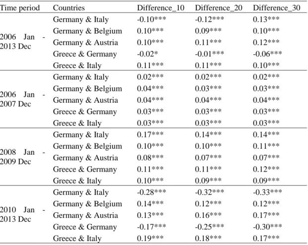
In following table, we report the average of difference between two correlation coefficient measures and also report the result of paired t tests. The null hypothesis of each paired t test is that the correlation coefficients between base point changes of two sovereign bonds equal the correlation coefficients between percentage changes of the VaR of those two sovereign bonds, ρ̂ij,t,bp− ρ̂ij,t,VaR= 0. *, **, and ***, mean to reject the null hypothesis at 10%, 5%, and

1% significant level, respectively.

In both measures, correlation coefficients are calculated by last 10, 20 and 30 days and report in Difference_10, Difference_20 and Difference_30, respectively.

Time period Countries Difference_10 Difference_20 Difference_30

2006 Jan - 2013 Dec

Germany & Italy -0.10*** -0.12*** 0.13*** Germany & Belgium 0.10*** 0.09*** 0.10*** Germany & Austria 0.10*** 0.11*** 0.12*** Greece & Germany -0.02* -0.01*** -0.06*** Greece & Italy 0.11*** 0.11*** 0.10***

2006 Jan - 2007 Dec

Germany & Italy 0.02*** 0.02*** 0.02*** Germany & Belgium 0.04*** 0.03*** 0.03*** Germany & Austria 0.04*** 0.04*** 0.04*** Greece & Germany 0.03*** 0.03*** 0.03*** Greece & Italy 0.03*** 0.03*** 0.03***

2008 Jan - 2009 Dec

Germany & Italy 0.17*** 0.14*** 0.14*** Germany & Belgium 0.10*** 0.10*** 0.11*** Germany & Austria 0.08*** 0.07*** 0.07*** Greece & Germany 0.11*** 0.11*** 0.12*** Greece & Italy 0.10*** 0.09*** 0.09***

2010 Jan - 2013 Dec

Germany & Italy -0.28*** -0.32*** -0.33*** Germany & Belgium 0.14*** 0.12*** 0.12*** Germany & Austria 0.13*** 0.16*** 0.17*** Greece & Germany -0.17*** -0.25*** -0.30*** Greece & Italy 0.19*** 0.18*** 0.17***

(14)

10

Even though, before 2008, the correlation coefficients between base point changes in bond yields and the correlation coefficients between percentage changes of VaR could track each other quite well as in Graph I to III of Figure 1, and we can still reject the null hypothesis as in Table 1, because the variances of those differences are also small.

After 2008, when the VaR of individual sovereign bonds is increasing and even soaring after 2010, we can observe that both correlation coefficient series fluctuate a lot as in Graph V (A) and V (B) of Figure 1, and the differences between those two correlation coefficients measures are always statistically different from 0.

Only one exception happens between Greece and Germany with the rolling window 10 days, where we can only reject the null hypothesis that the differences between the correlation coefficients measures equal 0 at 10% significant level. However, we reject the null hypothesis in any of the subsample, thus the failure of rejection is due to the increasing variance after 2008.

We can conclude that the correlation coefficients between base point changes in bond yields and the correlation coefficients between the percentage changes of the bonds’ VaR are significantly different from each other all the time. Hence, we should estimate the VaR of each security first, and then analyze the correlation coefficients between VaR of Greek sovereign bonds and another EMU sovereign bonds.

3. Choosing the appropriate VaR to measure tail risk

Even though the VaR is a commonly accepted way to measure the market risk, there are still some differences among VaR models and distributional assumptions. The majority of these differences falls into one of the following categories: i) the model to forecast variance; ii) the distribution of standard errors or returns; iii) the explanatory variables in the model.

Because of those differences, the VaR estimates obtained from different models can be very different from each other. Beder (1995) applied 8 common VaR methodologies to three hypothetical portfolios, and found that the estimated VaR from one model could as much as 14 times bigger than the VaR estimated with other models. At best there is an appropriate VaR model for each asset with a certain confidence level and at a certain time period. So, in this section, we

(15)

11

briefly review the existing VaR models and choose the appropriate VaR model for the EMU sovereign bond market using a comprehensive set of tests.

3.1 Brief summary of common VaR models

The most popular VaR models are parametric VaR models. The underlying assumption is that returns follow a parametric distribution with some determined parameters. The major differences among models are the parametric distribution in questions, and the way their parameters are estimated, in particular the variance.

In terms of methods to estimate the variance, the simplest method is equally weighted method. In this method, the current variance, 𝛔_𝐭𝟐, is estimated using the last k observations as follows.

{𝛔𝐭𝟐=

∑𝐭−𝐤−𝟏𝐭−𝟏 (𝐫𝐢− 𝟎)𝟐 𝐤

𝐫𝐭~ 𝐢. 𝐢. 𝐝. (𝟎, 𝛔𝐭𝟐)

(𝟐)

Usually, we assume the distribution of returns has zero mean and estimate the dynamic variance, σ_t2 by equation 2. Then we specify the distribution of rt, commonly standard normal or student t distribution, and the VaR at 99% confidence level (VaR99%) is equal to the 1st percentile of the profit and loss distribution.

The second method to estimate the variance is the GARCH model. ARCH models were first introduced by Engle (1982) and Bollerslev (1986) and gradually developed into a family of GARCH models, including, for example, the EGARCH introduced by Nelson (1991), the TGARCH introduced by Zakoian (1994) and the GJR introduced by Glosten et al (1993).

Even though GARCH (p, q) is theoretical reasonable, Bollerslev, Chou and Kroner (1992) proved that GARCH (1,1) as in equation 3 could already satisfy our needs in estimating the variance of financial data.

{ 𝐫_𝐭 = 𝛔_𝐭𝛆_𝐭 𝛆_𝐭~𝐢. 𝐢. 𝐝. (𝟎, 𝟏) 𝛔_𝐭𝟐 _{= 𝛃} 𝟎+ 𝛃𝟏𝐲𝐭−𝟏𝟐 + 𝛃𝟐𝛔𝐭−𝟏𝟐 𝐖𝐡𝐞𝐫𝐞 𝛃𝟎, 𝛃𝟏, 𝛃𝟐 > 𝟎, 𝛃𝟏+ 𝛃𝟐< 𝟏 (𝟑)

There are two critical assumptions in this model: the variance estimating equation is appropriate, and the standardized residuals are independent and identically distributed.

(16)

12

In addition, we need to specify the distribution of εt, commonly standard normal or student t distributions, in order to estimate the GARCH parameters by maximizing log-likelihood function. The VaR is then calculated as previously explained.

The third method to estimate the variance is Exponential Weighted Moving Average (EWMA) approach, which is a special empirical case of GARCH model and promoted by RiskMetrics introduced by a technology group of J.P. Morgan (1996).

{𝛔𝐭 𝟐_{= 𝛌𝛔} 𝐭−𝟏 𝟐 _{+ (𝟏 − 𝛌)𝐫} 𝐭−𝟏𝟐 𝐫_𝐭~𝐢. 𝐢. 𝐝. (𝟎, 𝛔_𝐭𝟐) (𝟒)

To estimate the variance, λ is usually set to a value of 0.94 or 0.97.5

As an alternative to the parametric VaR models, we have Historical VaR models. In these models, the underlying assumption is that returns follow the historical distribution.

The most basic method in this category is the simple historical simulation. In this method, we first choose a sample size, commonly from six months to two years. Then sort portfolio returns within this sample from the worst to the best returns and use (1 − θ) percentile as VaR_θ%. In this method, every observation within the window is given an equal weight, thus the estimations are biased, because of the changing volatility.

Boudoukh, Rishardson and Whitelaw (1998) proposed the Hybrid Historical Simulation to improve the simple historical simulation model.

In this method, each return in the sample, r_t, 𝑟_𝑡−1, 𝑟_𝑡−2… , is associated to a different exponentially decaying weight, 1−λ

1−λk, (

1−λ 1−λk) λ, (

1−λ 1−λk) λ

2_{, … The returns are sorted from the worst} to the best, and the VaR estimate is obtained by summing the corresponding weights until reaching 1 − θ% (one minus confidence level). In this method, Boudoukh, Rishardson and Whitelaw (1998) use 0.97 and 0.99 as λ.

In addition, Hull and White (1998) introduced the volatility adjusted historical simulation methods which adjust historical returns as in equation 5.

5_{Fleming, Kriby and Ostdiek (2001) found the optimal decay factor, λ, for daily time series data close to 0.94 and}

(17)

13

𝐫_𝐣,𝐭∗ = 𝛔𝐣,𝐓 𝐫_𝐣,𝐭 𝛔𝐣,𝐭

(𝟓)

where σ_j,T is the most recent GARCH/EWMA estimate of the daily standard deviation of returns, basing on available information at the end of day T-1; σ_j,t is the historical GARCH/EWMA estimate of the daily standard deviation of returns, basing on available information at the end of day t-1. After assuming the probability distribution of 𝑟_𝑗,𝑡⁄σ_j,t is stationary, we could replace historical returns (𝑟_𝑗,𝑡) by adjusted historical returns (𝑟_𝑗,𝑡∗ ), and then VaR_𝜃%,𝑇 equals 1 − θ% percentile of historical distribution of 𝑟_𝑗,𝑡∗.

As a third set of VaR models we have the Direct VaR models, which estimate the VaR directly from some explanatory variables. The most popular member of the Direct VaR model family is the Conditional Autoregressive VaR (CAViaR), introduced by Engle and Manganelli (2004). The CAViaR model directly forecasts the VaR over time, without specifying the distribution of returns as equation 6 shows.

𝐕𝐚𝐑𝐭,𝛉% = 𝛃𝟎+ 𝛃𝟏𝐕𝐚𝐑𝐭−𝟏,𝛉%+ 𝐥(𝛃𝟐, … , 𝛃𝐩, ; 𝛀𝐭−𝟏) (𝟔) where Ω_𝑡−1 is the information set available at time t.

However, all of previous models have their pros and cons.

First, the main advantage of parametric VaR models is that they allow the variance of financial returns to be varying across time, which is a generally accepted fact in financial market. Besides, we can obtain a complete characterization of the continuous distribution of financial returns, which can be used to estimate different risk measures, like expected tail loss, VaR at different confidence level and semi-variance. On the other hand, equally weighted method, GARCH and RiskMetrics models are all subject to three sources of misspecifications: i) the variance estimating equation could be misspecified; ii) the distribution of standardized residuals chosen to build log-likelihood function could be wrong; iii) the standardized residuals may not be independent and identically distributed. In addition, even though we could have better flexibility on tails by using a student t distribution or a generalized error distribution rather than a normal distribution, the limited number of observations on tails and the outliers would reduce the accuracy of the tail estimation.

(18)

14

When comparing with parametric VaR models, historical simulation do not need a specific distribution of returns and historical distribution has a naturally negative skewness and higher kurtosis than normal distribution, but both simple historical simulation and Hybrid Historical Simulation cannot reflect current market volatility. Because of the drawback in adjusting dynamic market volatility of historical simulation methods, Hull and White (1998) proposed the volatility adjusted historical simulation method, and proved that this method could outperform simple historical simulation and Hybrid Historical Simulation when estimating VaR at 99% confidence level, using the historical data of foreign exchange market and equity market.

Direct VaR models are straight forward, but they reply on a complete set of independent variables, which could be varied from market to market and even from time to time.

Since we do not have enough empirical results to support a direct VaR model to estimate sovereign bonds and Hull and White(1998) proved that volatility adjusted historical simulation could outperform other historical VaR models, in this paper, we compare several parametric models (RiskMetric, GARCH and GJR model) with corresponding volatility adjusted historical simulations to test whether volatility adjusted historical simulation could also outperform the parametric methods and to choose an appropriate model to estimate VaR at 99% confidence level in EMU sovereign bond market.

In sovereign bond market, investors could easily access the base point changes of bond yields instead of the returns in equity market, thus we usually use Present Value of a base point decrease (PV01) as risk exposure and adjust VaR estimation process as follows.6 If we want to estimate VaR_{𝑖,99%,𝑡}, first we need to estimate the 99th percentile of recent base point changes of country i’s sovereign bond yield using a parametric method or a volatility adjusted historical simulation.7 Then we calculate VaR_{𝑖,99%,𝑡} by multiplying the risk exposure (-PV01), as equation 7 shows.

6_{For daily data, the first derivative of the Present Value versus interest rate would be a good approximation for}

PV01, present value of 1 base point change, since the daily base point changes are quite small. PV01(CT, RT) ≈

∂PV(CT, RT)

∂RT

× −1 b. p = −T × PV(CT, RT) × −0.01%

7_{Present value of sovereign bond will decrease if interest rate increases. Thus, sovereign bond will have extreme}

loss if the base point change has an extremely positive value. We need to replace financial returns (r𝑗,𝑡) of the

original volatility adjusted historical simulation proposed by Hull and White (1998), by base point changes (bp𝑗,𝑡)

(19)

15

𝐕𝐚𝐑_𝐢,𝐭= − 𝐢𝐧𝐟(𝐛𝐩_𝐢,𝐭) × −𝐏𝐕𝟎𝟏 (𝟕)

where inf (. ) is the inverse of Probability Density Function; bp_𝑖,𝑡 is the base point change of security i at time t; PV01 is the Present Value change if the interest rate decreases 1 base point.

Besides, we also make following assumptions in our analysis. First, interest rates are continuous compounding8. Second, to standardize the VaR and increase the comparability, our risk exposure (PV01) is equal to 100 in all the sovereign bonds. Third, our positions are rebalanced every day, which means we will rebalance the amount of investments every day to maintain a constant PV01, 100.

3.2 Battery of back testing methods

In order to determine which of the VaR models is the most appropriate for the EMU sovereign bond market, we use a battery of back tests. After completing all tests, we assign a punishment score to each rejection of the validity or independence test, and sum up the punishment scores for each VaR model. In the end, we form a punishment scorecard and choose the VaR model based on the total punishment scores. By doing this, even though we have to set some subjective criteria when forming the scorecard, we could make a relatively objective decision when choosing among VaR models. If we consider some tests to be more important than others, we can simply assign a higher punishing score to them.

We will consider the following five validity and independence tests in our back testing battery: i) the Unconditional Coverage test; ii) the Independence test; iii) the Conditional Coverage test; iv) the Berkowitz, Christoffersen and Pelletier (2007) test (henceforth BCP test); and v) the Unconditional Exceedance Clustering test.

The null hypothesis of the Unconditional Coverage test, introduced by Kupiec (1995), is that the observed exceedance rate equals the expected exceedance rate.

We expect the probability of the exceedance rate (there is an exceedance if the absolute value of the loss of the security is larger than estimated VaR) equals one minus confidence

8_{We have transformed the interest rate from annual compounding or semi-annual compounding into continuous}

compounding. All the interest rates of the generic sovereign bonds, except Italian sovereign bonds, are annually compounded. The interest rates of Italian sovereign bonds are semiannual compounded.

(20)

16

level, (1 − θ%), all the time, if the VaR model is appropriate. The loglikelihood ratio test statistic is calculated according to equation 8.

𝐋𝐑_𝐮𝐜 = (𝛑𝐞𝐱𝐩 𝛑_𝐨𝐛𝐬) 𝐧𝟏 (𝟏 − 𝛑𝐞𝐱𝐩 𝟏 − 𝛑_𝐨𝐛𝐬) 𝐧𝟎 (𝟖)

where π_exp is the expected exceedance rate, and equals one minus the confidence level (1 − θ%), 𝜋_𝑜𝑏𝑠 is the observed exceedance rate, n₁ is the number of exceedance, n₀ is the number of non-exceedances. Based on the test statistic (LRuc), we have that −2ln (LRuc)~χ2(1) and so we can check whether the null hypothesis is rejected by comparing −2ln (LR_uc) against the appropriate critical value of the chi-square distribution with 1 degree of freedom.

The null hypothesis of the Independence test, derived by Christoffersen (1998), is that the exceedances are independent from each other.

The Independent test is based on the notion that if exceedances are independent, the probabilities of exceedance of nest interest rate is not related to what happens before that.

𝐋𝐑𝐢𝐧𝐝 = 𝝅_𝒐𝒃𝒔𝒏𝟏 (𝟏 − 𝝅_𝒐𝒃𝒔)𝒏𝟎 𝝅_𝟎𝟏𝒏𝟎𝟏_{(𝟏 − 𝝅} 𝟎𝟏)𝒏𝟎𝟎𝝅𝟏𝟏 𝒏𝟏𝟏_{(𝟏 − 𝝅} 𝟏𝟏)𝒏𝟏𝟎 (𝟗)

where, n10(𝑛11) is the number of exceedances followed by a non-exceedance (exceedance), n₀₀(𝑛₀₁) is the number of non-exceedances followed by a non-exceedance (exceedance), π₀₁ =

n01

𝑛01+𝑛00 and π11=

n11

𝑛11+𝑛10. We also have −2 ln(LRind) ~χ

2_{(1), thus we need to check whether we} will reject the null hypothesis by comparing −2 ln(LR_ind) against the appropriate critical value of the chi-square distribution with 1 degree of freedom.

The null hypothesis of Conditional Coverage test, also proposed by Christoffersen (1998), is that the observed exceedance rate equals the expected exceedance rate and the exceedances are independent from each other.

𝐋𝐑_𝐜𝐜 = 𝛑𝐞𝐱𝐩 𝐧𝟏 _{(𝟏 − 𝛑} 𝐞𝐱𝐩) 𝐧𝟎 𝛑_𝟎𝟏𝐧𝟎𝟏_{(𝟏 − 𝛑} 𝟎𝟏)𝐧𝟎𝟎𝛑_𝟏𝟏𝐧𝟏𝟏(𝟏 − 𝛑𝟏𝟏)𝐧𝟏𝟎 (𝟏𝟎)

(21)

17

Since the asymptotic distribution of −2 ln(LRcc) follows a chi-square distribution with 2 degree of freedom, we could check whether we should reject the null hypothesis by checking chi-square test table.

Since both Independent test and Conditional Coverage test could only find out the exceedance clustering problem if exceedances are consecutive, we also include the BCP test, introduced by Berkowitz, Christoffersen and Pelletier (2007) to test higher order exceedance clustering problem.

The null hypothesis of the BCP test is that the exceedances are independent at K order.

𝐁𝐂𝐏(𝐊) = 𝐧(𝐧 + 𝟐) ∑ 𝛒̂𝐤 𝟐 𝐧 − 𝐤 𝐊 𝐤=𝟏 (𝟏𝟏)

where n is sample size; k is the autocorrelation lag considered in the test; 𝜌̂_k = Corr(I_t,α− α, I_t+k,α− α) is the lag k sample autocorrelation of the series I_t,α− α;

I_t,α− α = {1 𝑖𝑓 𝑃𝑟𝑜𝑓𝑖𝑡 𝐿𝑜𝑠𝑠 < −𝑉𝑎𝑅𝑡,𝛼

0 𝑜𝑡ℎ𝑒𝑟𝑤𝑖𝑠𝑒 is the exceedance indicator.

As an asymptotic test, we have 𝐵𝐶𝑃(𝐾)~ χ2(𝑘), so we could test whether the null hypothesis should be rejected based on BCP statistic and chi-square distribution with k degree of freedom.9

Since all of previous tests could only detect the consecutive independence problem, we also adjust the Unconditional test, named as the Unconditional Exceedance Clustering test, to examine whether the exceedances are clustering at a certain variance level.

The null hypothesis of the Unconditional Exceedance Clustering test is that the observed exceedance rate in each variance decile group equals the expected exceedance rate.

We sort the whole sample by estimated variance and group the whole sample into ten quantile,10 basing on the decile breakpoints for estimated variance. Then we implement the Unconditional tests on each variance group as equation 8 shows.

3.3 The Punishment Scorecard

9_{We will test whether there is higher order (until K=5 order) autocorrelation of exceedances in this thesis.} 10_{For instance, VaR with lowest 0% to 10% variance belongs to group 1; VaR with lowest 10% to 20% variance}

(22)

18

To quantify the performance of VaR models, we use a scorecard to summarize the performance of VaR models in each of the five tests.

We test the VaR models annually for each country, and for the entire sample period in each test. In Unconditional Coverage, Independence and Conditional Coverage tests, each VaR model has 8 annual test results and 1 total test result for each country; in BCP tests, each VaR model has 40 annual test results (we will test autocorrelation from 1st_{order to 5}th_{order annually) and 5 total test} results; and Unconditional Exceedance Clustering tests have 10 group test results (1 test for each decile group) for each country.

According to the null hypotheses of each test, there are three kinds of problems that make us reject the VaR model: i) the observed exceedance rate is not equal to the expected exceedance rate; ii) the exceedances are not independent from each other, because the VaR model is not sensitive enough to capture changes in market conditions; iii) The exceedances are clustering in some variance groups.

Since the Unconditional tests are the elementary tests for the validity, we give them the most severe punishment scores. Considering that Unconditional tests, Conditional tests and Unconditional Exceedance Clustering tests have overlaps in testing the validity, we give two latter tests relatively low punishment scores. Besides, since we have lots of BCP tests in each country and the rejections of BCP tests for high order autocorrelation problem seem questionable at a high confidence level, so we give them the lowest punishment score per rejection. Also, both Independent and Conditional tests could test independence, and their punishment scores are relatively low because of the overlaps.

After those subjective judgements, we pay almost equal attention to the problem (i) that the observed exceedance may not fit our expectation and the problem (ii) that exceedances are not independent, and put less weight on the last problem that the exceedances are clustering in some variance groups, since Alexander (2009) suggested that the first two problems are the key aspects of the VaR tests.

In any of five tests, if a p value is smaller than 5% but bigger than 1%, the VaR model will receive a punishment score, but if a p value is smaller than 1%, the VaR model will receive a more severe punishment score as table 2 shows.

(23)

19 Table 2. The Punishment Scorecard.

We give different punishment scores to each rejection basing on the importance of tests and potential overlapping among tests. Besides, we also differentiate the punishment score per rejection under 1% and 5% significant level, since the probabilities of making type I and type II error are quite different between those two significant levels. Following table lists the detailed punishment score per rejection in different test and significant level in the thesis.

p value 1%~5% <1%

Unconditional Tests annual 2/rejection 4/rejection total 6/rejection 12/rejection Independent Tests annual 2/rejection 4/rejection

total 4/rejection 8/rejection Conditional Tests annual 2/rejection 4/rejection total 4/rejection 8/rejection

BCP Tests annual11 _1/rejection _2/rejection

total 2/rejection 4/rejection Unconditional Tests(clustering) decile group12 _2/rejection _4/rejection

The objective of this scorecard is to quantify the performance of VaR models.

According to the final scorecard, we can qualify the performance of VaR models and find the most efficient VaR model to estimate the tail risk of each sovereign bond market.

Even though we have to make some subjective assumptions in the beginning, it’s better to make a sound decision based on subjective assumptions rather than make a totally subjective decision based on dozens of test results.

3.4 Data

We use 5 year Generic Government Rates between Jan 1st_{2003 and Dec. 31}st_{2013 obtained} from Bloomberg as 5 year sovereign bond yield during that period. Since we use first three years data to stabilize EWMA model, we just estimate VaR between 2006 and 2013. The countries covered in the sample are Austria, Belgium, France, German, Greece, Italy, Netherlands, Portugal and Spain.13 We have also included relevant financial data, such as the implied volatility of S&P

11_{If we don’t have any exceedance in a sovereign bond market for one year, we will reject all the BCP tests for that}

year. However, we do not count those meaningless rejections.

12_{The total tests of unconditional tests (clustering) are identical to total tests of unconditional tests.}

13_{5 year Greek government debt data is only available before Mar 13}th_{2012. In Mar. 13}th_{2012 Fitch raised Greek}

(24)

20

500 index options (VIX), and local equity indexes (ATX, BEL20, OMX Helsinki 25, CAC40, DAX, Athex20, ISEQ20, FTSE MIB, AEX index, PSI 20 and IBEX 35) from Bloomberg as global and local factors. The last global factor, the USD/EUR exchange rate, is obtained from FactSet and priced in the US exchange rate method.14

To match the data from different countries and different markets, we only consider data during working days. If the data is not available in Bloomberg or FactSet, we use simple average method to interpolate the missing data.15_{As in Appendix 1, all EMU countries included in this study have} almost completed series of 5 year Generic Government rates, and just need sporadic interpolations.

We can see from Table 3, for any EMU country, the mean of base point changes is not significantly different from 0. Even though the mean of base point change in the Greek sovereign bond market is relatively big (2.7626), the variance of the Greek sovereign bond market is also large (1293.524).

Table 3: Basic Momentum summary

Following table lists basic statistic momentums of different 5 year EMU sovereign bonds between Jan 1st_{2003 and}

Dec. 31th 2013.

Austria Belgium France Garman Greece Italy Netherland Portugal Spain mean -0.08152 -0.08337 -0.08539 -0.10082 2.762661 -0.01861 -0.08634 0.089466 -0.01472 Variance 27.40989 34.24749 26.23718 25.49652 1293.524 81.27417 23.9539 381.8136 82.02864 Skewness 0.533176 -0.01204 0.300469 0.079468 -2.47737 -0.86225 0.200142 1.56018 -1.26961 Excess kurtosis 6.270829 10.21717 3.884917 1.959229 75.20575 18.4382 2.256182 58.45064 16.16104

Also, we can see base point changes are not stationary in any of EMU countries from Appendix 2. To be specific, the variances of base point changes are not constant. Thus, it is necessary to find an appropriate model, EWMA or GARCH, to estimate dynamic variance so we consider parametric VaR models and volatility adjusted historical simulation in this thesis.

3.5 VaR models and scorecard results

maturity, for instance 10 year and 30 year, decreased dramatically, and yield to maturity of 5 year Greek sovereign bond was not available in Bloomberg for one year.

14_{This exchange rate is priced as the amount of dollars needed to purchase one unit of euro.} 15_{If i}

j,t, which is the interest rate of sovereign bond market j, at time t, is missing, we will interpolate the missing

data by ij,t=

i_j,t−1+i_j,t+1 2

(25)

21

Nine different VaR methods are used to estimate the tail risks: three RiskMetrics models, four

ARMA (1,0)-GARCH(1,1) models and two ARMA(1,0)-GJR(1,1,1) models.

Model Norm uses EWMA to estimate daily variance and assume that the standardized base point changes (εj,t) follow normal distribution as in equation 12

{𝛔𝐣,𝐭 𝟐 _{= 𝛌𝛔} 𝐣,𝐭−𝟏 𝟐 _{+ (𝟏 − 𝛌)𝐛𝐩} 𝐣,𝐭−𝟏 𝟐 𝐛𝐩_𝐣,𝐭= 𝛔_𝐣,𝐭𝛆_𝐣,𝐭 𝛆_𝐣,𝐭~𝐢. 𝐢. 𝐝. 𝐍(𝟎, 𝟏) (𝟏𝟐)

where bpj,t is the base point change of sovereign bond j at time t; σj,t is the standard deviation of sovereign bond j at time t; εj,t is standardized base point change of sovereign bond j at time t, in short it is the standard error of sovereign bond j at time t. And λ = 0.94 according to Fleming, Kriby and Ostdiek (2002). 16

Model S.t uses EWMA to estimate daily variance and use maximizing the log-likelihood function approach to estimate the degree of freedom of student t distribution of standardized base point changes (εj,t) as in 13 { 𝛔_𝐣,𝐭𝟐 = 𝛌𝛔_{𝐣,𝐭−𝟏}𝟐 + (𝟏 − 𝛌)𝐛𝐩_{𝐣,𝐭−𝟏}𝟐 𝛌 = 𝟎. 𝟗𝟒 𝐛𝐩_𝐣,𝐭= 𝛔_𝐣,𝐭𝛆_𝐣,𝐭 𝛆_𝐣,𝐭~𝐢. 𝐢. 𝐝. 𝐬𝐭𝐮𝐝𝐞𝐧𝐭 𝐭(𝟎, 𝟏) (𝟏𝟑)

Model His, 500 is a volatility adjusted historical simulation, in which variance is adjusted by EWMA method, as in 14. And the 99th percentile of base point changes distribution is estimated by last 500 volatility adjusted base point changes in bond yields.

{ 𝛔𝐣,𝐭𝟐 = 𝛌𝛔𝐣,𝐭−𝟏𝟐 + (𝟏 − 𝛌)𝐛𝐩𝐣,𝐭−𝟏𝟐 𝛌 = 𝟎. 𝟗𝟒 𝐛𝐩_𝐣,𝐭∗ = 𝛔_𝐣,𝐓𝐛𝐩𝐣,𝐭 𝛔_𝐣,𝐭 (𝟏𝟒)

where T indicates the target time when we want to estimate the 99th percentile of the adjusted base point changes distribution, and t indicates historical observations t~[T − 1, T − 500]

16_{We also estimate λ by assumption that all the standardized base point change follow same distribution. We can}

get λ =0.948445 by minimizing variance of momentums, mean, variance, excess kurtosis and skewness. Thus, λ = 0.94 is suitable here.

(26)

22

In GARCH models and GJR models, we cannot assume the base point changes have zero conditional means, since the basic requirement of GARCH model is the mean of standard errors, v_j,t, equals 0. Thus, we use ARMA(1,0) model to estimate conditional means.

Model G, Norm uses ARMA (1,0)-GARCH(1,1) as in 15 and the additional assumption that standardized base point changes (ε_j,t) follow normal distribution.

{ 𝐛𝐩_𝐣,𝐭 = 𝛂_𝟎+ 𝛂_𝟏𝐛𝐩_{𝐣,𝐭−𝟏}+ 𝐯_𝐣,𝐭 𝐯𝐣,𝐭= 𝛔𝐣,𝐭𝛆𝐣,𝐭 𝛆𝐣,𝐭~𝐢. 𝐢. 𝐝. 𝐍(𝟎, 𝟏) 𝛔_𝐣,𝐭𝟐 = 𝛃𝟎+ 𝛃𝟏𝐯𝐣,𝐭−𝟏𝟐 + 𝛃𝟐𝛔𝐣,𝐭−𝟏𝟐 𝛃_𝟎, 𝛃_𝟏, 𝛃_𝟐 > 𝟎, 𝛃_𝟏+ 𝛃_𝟐< 𝟏 (𝟏𝟓)

Model G, N, His is another volatility adjusted historical simulation, in which variance is estimated by ARMA (1, 0)-GARCH (1, 1) model as in equation 15 and historical base point changes in bond yields are adjusted by the variances as equation 16 shows. The 99th percentile of base point changes distribution is estimated by last 500 adjusted base point changes in bond yields.

𝐛𝐩_𝐣,𝐭∗ = 𝛂𝟎+ 𝛂𝟏𝐛𝐩𝐣,𝐭−𝟏+ 𝛔𝐣,𝐓 𝐯_𝐣,𝐭 𝛔𝐣,𝐭

(𝟏𝟔)

Model G, S.t uses ARMA (1, 0)-GARCH (1, 1) and the additional assumption that standardized base point change follow student t distribution as in equation 17 to estimate daily variance.

{ 𝐛𝐩𝐣,𝐭 = 𝛂𝟎+ 𝛂𝟏𝐛𝐩𝐣,𝐭−𝟏+ 𝐯𝐣,𝐭 𝐯_𝐣,𝐭 = 𝛔_𝐣,𝐭𝛆_𝐣,𝐭 𝛆_𝐣,𝐭~𝐢. 𝐢. 𝐝. 𝐬𝐭𝐮𝐝𝐞𝐧𝐭 𝐭(𝟎, 𝟏) 𝛔_𝐣,𝐭𝟐 = 𝛃_𝟎+ 𝛃_𝟏𝐯_{𝐣,𝐭−𝟏}𝟐 + 𝛃_𝟐𝛔_{𝐣,𝐭−𝟏}𝟐 𝛃𝟎, 𝛃𝟏, 𝛃𝟐 > 𝟎, 𝛃𝟏+ 𝛃𝟐 < 𝟏 (𝟏𝟕)

Model G, S.t, His uses equation 17 to estimate daily variance, and adjust historical base point changes as in equation 16.

Model GJR uses ARMA (1,0) − GJR (1,1,1) and the assumption that standardized errors (ε_j,t) are normally distributed to estimate variance and VaR.

{ 𝐛𝐩_𝐣,𝐭 = 𝛂_𝟎+ 𝛂_𝟏𝐛𝐩_{𝐣,𝐭−𝟏}+ 𝐯_𝐣,𝐭 𝐯_𝐣,𝐭 = 𝛔_𝐣,𝐭𝛆_𝐣,𝐭 𝛆_𝐣,𝐭~𝐢. 𝐢. 𝐝. 𝐍(𝟎, 𝟏) 𝛔_𝐣,𝐭𝟐 = 𝛃_𝟎+ 𝛃_𝟏𝐯_{𝐣,𝐭−𝟏}𝟐 + 𝛃_𝟐𝛔_{𝐣,𝐭−𝟏}𝟐 + 𝛃_𝟑𝐯_{𝐣,𝐭−𝟏}𝟐 (𝐢𝐟 𝐯_{𝐣,𝐭−𝟏} > 𝟎) 𝛃𝟎, 𝛃𝟏, 𝛃𝟐 > 𝟎, 𝛃𝟏+ 𝛃𝟐 < 𝟏 (𝟏𝟖)

(27)

23

Model GJR, His is GJR volatility adjusted historical simulation, which use equation 18 to estimate variance and equation 16 to adjust historical base point changes.

According to Panel I and II of Table 4, we find that His, 500 model (EWMA volatility adjusted historical simulation) has the lowest punishment score in any single tests and the lowest total punishment score.17

First, S.t (RiskMetrics model with student t distributed ε_j,t) has better performance than Norm (RiskMetrics model with normal distributed ε_j,t) (Total punishment score is 84 in S.t and 348 in Norm, and S.t has less rejectctions in any of the five tests than Norm). Thus the real distribution of standardized base point changes has fatter tail, since student t distribution are more flexible on tails than normal distribution. Besides, there are two reasons to explain the fact that historical simulation could improve the performance further: i) there is a limited number of observations on tails; ii) standardized base point changes are asymmetrically distributed. Even though student t distribution has good flexibility on tails, there are not enough number of observations to estimate the tails accurately. Or the real distribution of standardized base point changes is not symmetric, thus a symmetric distribution is not a wise choice, as Table 4 shows.

Second, His, 500 model beats all the GARCH models. This might be due to three possible explanations. Frist, coefficients of GARCH models are heavily influenced by outliers, thus biasing the varaince estimation. Second, those coefficients are not constant. Third, conditional means tend to be 0 rather than follow ARMA(1,0) model.

We also find that G,S.t (GARCH model with student t distributed ε_j,t) model tends to overestimate the VaR all the time. Even though the student t distribution has fatter tail compared to the normal distribution, it will overestimate daily VaR_𝑖,𝑡, at 99% confidence level. This means that the flexibility in the tails cannot increase the accuracy of variance estimation, because of the influence of outliers and the limited number of observations on the tails.

In addition, the GJR model cannot significantly improve estimations of VaR_j,t,1,99% compared to the model G, Norm (GARCH model with normally distributed ε_j,t).

17_{In model Norm and His,500,our test results are out of sample tests’ results, since we do not need any future}

(28)

24 Table 4, Brief summary of back tests

Panel I reports the number of rejections in each test at different significant level. We will exclude the rejections in annual BCP tests if those rejections are caused by absence of exceedance during that year. We also exclude the total Unconditional Exceedance Clustering test, since it is idential to total Unconditional Coverage test.

After multipling corresponding punishment score as in Table 2 and summing up punishment scores in each tests we summarize total punishment scores in each tests and total punishment scores of five tests, and report in Panel II.

Panel I Number of rejection in each test

Panel II Punishment Scorecard results

Norm S.t His,500 G,Norm G,S.t GJR G,N,His G,S.t,His GJR,His

Unconditional Tests 164 20 6 140 252 148 18 36 18 Independent Tests 10 0 0 0 0 4 0 0 0 Conditional Tests 10 0 0 0 0 4 0 0 0 BCP Tests 82 42 42 81 180 74 51 51 48 Unconditional Exceedance Clustering test 82 22 18 48 180 34 30 32 28 Total Score 348 84 66 269 612 264 99 119 94

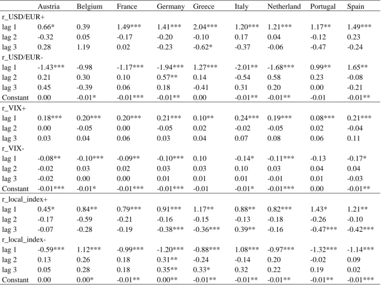
As Table 5 shows, even though 6 out of 10 countries’ sovereign bond markets have statistic significant asymmetric items in GJR(1,1,1) model at 5% significance level as in Table 5, the sign of coefficients of some countries cannot fit our expectation that bad news has more impact than good news. Besides, GJR model only improve total punishment score moderately (269 in G,Norm

Norm S.t His,500 G,Norm G,S.t GJR G,N,His G,S.t,His GJR,His Unconditional Coverage test Annual 1%~5% 8 8 3 8 72 11 3 4 5 <1% 10 1 0 7 0 6 3 4 2 Total 1%~5% 0 0 0 2 0 1 0 0 0 <1% 9 0 0 7 9 8 0 1 0 Independent test Annual 1%~5% 3 0 0 0 0 0 0 0 0 <1% 0 0 0 0 0 1 0 0 0 Total 1%~5% 1 0 0 0 0 0 0 0 0 <1% 0 0 0 0 0 0 0 0 0 Conditional Coverage test Annual 1%~5% 3 0 0 0 0 0 0 0 0 <1% 0 0 0 0 0 1 0 0 0 Total 1%~5% 1 0 0 0 0 0 0 0 0 <1% 0 0 0 0 0 0 0 0 0 BCP test Annual 1%~5% 4 2 0 5 0 4 3 3 2 <1% 27 8 13 21 0 23 10 11 13 Total 1%~5% 2 2 2 1 0 2 0 1 0 <1% 5 5 3 8 45 5 7 6 5 Unconditional Exceedance Clustering test Differe nt decile 1%~5% 13 11 7 8 90 9 7 8 10 <1% 14 0 1 8 0 4 4 4 2

(29)

25

model, 99 in G,N,His model, 254 in GJR model, and 94 in GJR, His model). As a conclusion, the advantage of asymmetric GARCH model is not obvious when estimating variance in this data set.

Table 5, Asymmetric items in GJR(1,1,1) model

In GJR(1,1,1) model, we assume that good news and bad news have different influence on variance of base point changes as in following equation.

{

bpj,t= α0+ α1bpj,t−1+ vj,t

vj,t= σj,tεj,t εj,t~i. i. d. N(0,1)

σj,t2 = β0+ β1vj,t−12 + β2σj,t−12 + β3vj,t−12 (if vj,t−1> 0)

β0, β1, β2> 0, β1+ β2< 1

Since the spot interest rate and the price of an existing sovereign bond are negative correlated, β3, named as Tarch

Stat in following table, will report the additional effects of bad news. Following table report the coefficients and p value of the asymmetric item, β3 in different 5 year sovereign bond between 2006 and 2013.

Austria Belgium France Germany Greece Italy Netherland Portugal Spain Tarch Stat -0.03 0.00 -0.02 -0.01 0.13 0.09 -0.02 0.08 0.04 P Value 0.00 0.68 0.06 0.11 0.00 0.00 0.00 0.00 0.00

Third, the volatility adjusted historical simulation could improve the performance in all of parametric models (total punishing score is 269 in G,Norm versus 99 in G,N,His, 1332 in G,S.t versus 119 in G,S.t,His, 264 in GJR versus 94 in GJR,His)

As a conclusion, model His,500(EWMA) beats all the other models, with the smallest total pubishment score and individual punishment scores.18 Besides, we also find that volatility adjusted historical simulation could improve the performance of parametric VaR models.

4. Correlation Coefficients Analysis 4.1 The DCC model and data

There are three objectives in this section: find a potential pattern of the correlation coefficients between the Greek 5 year sovereign bond market and other major EMU 5 year sovereign bond markets; test whether this pattern is consistent among different time periods, especially before and after the Sovereign Bond Crisis; test whether the impact of Greece is the same on vulnerable

18_{Since in this paper, we need to estimate VaR}

1,99%,t rather than forecast VaR1,99%,t, we don’t need to distinguish in

sample tests and out of sample tests. However, commonly in sample tests’ results will be better than out of sample tests’ results. In this paper, surprisingly, out of sample tests’ results from His, 500 beat all the out of sample tests’ and in-sample tests’ results.

(30)

26

countries (Greece, Italy, Ireland, Portuguese and Spain) and stable countries (Austria, Belgium, France, Germany and Netherland).19

Nevertheless, the convergence problem caused by the existence of outliers and flatness of likelihood function, and the riskiness of reaching a local optimum stops us from including all the vulnerable and stable countries into a Multivariate GARCH model, thus, in this section, we focus on the dynamic correlation coefficients between Greece and other EMU top economic entities.

According to Gross Domestic Product (GDP), published by the World Bank, Germany, France, Italy and Spain were top 4 economic entities in the EMU from 2006 to 2013. But, the VaR of German and French 5 year sovereign bonds were quite stable during the entire period; on the contrary, the VaR of Italian, Spanish, and Greek 5 year sovereign bonds increased dramatically between 2008 and 2011, so the Multivariate GARCH model will suffer a convergence problem if we include all those four countries’ sovereign bonds. As a result, we use Italy and Spain to represent vulnerable countries and France to represent stable countries. 20

In addition, we also adjust the sample size in section 4 and section 5, since data series of Greek 5 year sovereign bonds is not available in Bloomberg after Mar. 12th 2012, when the majority of private holders agreed to participate the restructuring of Greek sovereign bonds. Besides, not until Apr. 11th 2014, did Greek 5 year sovereign bonds come back to financial market. Thus, the sample period would be from Jan. 1st 2006 to Dec. 31st 2011.

To obtain dynamic correlation coefficients, we apply the Dynamic Conditional Correlation (DCC) model, which was first introduced by Engle (2002) and is a simplified extension of traditional Multivariate GARCH model. The DCC model has become the main methodology to identify the volatility spillover between countries. For instance Celik (2012) used it to analyze the volatility spillover effects in emerging markets, and Elkhaldi and Chebbi (2013) used it to analyze the volatility spillover effects between different EMU countries. In this analysis, we will use STATA’s built-in function, which is calculated as in equation 19.

19_{Since Cyprus, Estonia, Latvia, Slovakia and Slovenia joined EMU very late, and data series of Generic}

Government rates of Luxembourg and Malta are not available in Bloomberg, we exclude those countries from our analysis.

20_{The convergence problem still exists if we only include German, Italian, Spanish and Greek 5 year sovereign}

Does contagion really matter: real role of Greece in the sovereign bond crisis