Vertical transfers and the appropriation of resources by the bureaucracy: the case of Brazilian state governments

(1)

VERTICAL TRANSFERS AND THE APPROPRIATION OF RESOURCES BY THE BUREAUCRACY: THE CASE OF BRAZILIAN STATE GOVERNMENTS

João Silva Moura Neto Getúlio Vargas Foundation School of Business - CEPESP IMAPES ESAMC Nelson Marconi Getúlio Vargas Foundation School of Business and Economics - CEPESP Pontifical Catholic University – São Paulo Paulo Eduardo Moledo Palombo Getúlio Vargas Foundation School of Business - CEPESP UniFECAP Paulo Roberto Arvate Getúlio Vargas Foundation School of Business and Economics -CEPESP Abstract

The Brazilian grant system was built by the federal government aiming to reduce economic and social inequalities in the federation, by transferring income from rich states to poor states. However, due to the lack of control and mechanisms for assessing the use of this public resource, these transfers may be appropriated by the bureaucracy as wage increases, for example. In order to observe this appropriation, we use the wage differential between the public and private sector in the states as a proxy, which is calculated using the technique developed by Oaxaca (1973). We do not use the ratio between wage expenses and total current expenses as proxy, because the results of this measure show no significant differences between rich and poor states. Our initial estimation was made with yearly panel data from 1995 to 2004, using the least squares dummy variables method (LSDV).

JEL: H71, H77

Key words: Vertical transfers, bureaucracy, public-private wage differential. Resumo

O sistema de transferências estruturado pelo governo federal visa reduzir as disparidades econômicas e sociais na federação através da transferência de renda dos estados mais ricos para os mais pobres. Entretanto, dada a ausência de controles e mecanismos que permitam a identificação do uso destes recursos públicos, estas transferências podem ser apropriadas pela burocracia na forma de aumentos salariais, por exemplo. Com o intuito de analisar esta apropriação, adotamos os diferenciais de salário entre o setor público e privado nos estados como uma proxy, os quais foram calculados usando a técnica desenvolvida por Oaxaca (1973). Nós não adotamos a relação entre gastos com pessoal e despesas correntes porque os resultados deste cálculo não indicaram diferenças significativas entre estados pobres e ricos. Nossa estimativa inicial foi feita a partir de dados de painel anuais, para o período entre 1995 e 2004, usando o método de mínimos quadrados com variáveis dummy.

(2)

1. Introduction

The grant system developed in Brazil in order to transfer resources from the richest to the poorest states via the federal government seems to be inefficient when it comes to correcting existing regional differences. One reason, analyzed in this paper, is that the resources sent to the poorest states can be appropriated by the bureaucracy as wage increases. Despite the weak empirical evidence between the wages of the bureaucrats and the level or growth rate of the budget they control1, we can see that the transfer system, which aims to minimize regional differences, lacks criteria when it comes to evaluating the efficiency of expenditure in Brazil. 2

The purpose of this study is to show that these transfers support the higher wages paid to state bureaucrats, when compared with the wages in the private sector. In order to achieve this purpose this paper has a further five sections in addition to this introduction. In the second section we provide a brief account of the evolution of the literature on bureaucracy, showing how important it is for monitoring purposes to know about and to compare the relative performances of the public and private sectors, considering the problem caused by the information asymmetries between the sponsor and the bureaucrat. In the third section we show the Brazilian vertical transfer system. In the fourth section we discuss expenditure on wages in state governments and its relationship with the preferences of the bureaucrats. We also present the calculation of the wage differentials for regions using the Oaxaca decomposition (1973). It is possible to observe that states in poor regions have a clear tendency to pay higher public sector wages when compared to private sector equivalents in same region. In the fifth section we present the model and the empirical tests to verify the impact of transfers on the wage premium for public employees. In the last section we present the main conclusions of this paper.

2. Theoretical aspects relating to the role of bureaucracy and some performance measures between the public and private sectors.

It is not an idea new to literature to highlight the role of bureaucracy within the state. The first systematic effort to study bureaucracy within the public sector was the one made by Niskanen (1971). This first effort was certainly influenced by the writings of Tullock (1965) and Downs (1967), although one can clearly see that they studied the different aspects of bureaucratic organizations still using an economic methodology.

All the developments of Niskanen (1971) were based on information asymmetries between bureaucrats and their funders-sponsors (politicians) in relation to the costs for producing the goods to be supplied by the bureau. Bureaucrats have better information on the costs for supplying the product than their funders. Funders and bureaucrats have a bilateral monopoly relationship, because bureaucrats sell their products only to the government and the government (the funder of the bureaucracy) receives the product from bureaucrats in exchange for a budget. Therefore, bureaucrats try to maximize their budget, subject to the restriction that the total budget must be equal to or higher than the production

1_{See Johnson and Libecap (1989) and Young (1991).}

2_{Australia and New Zealand, for example, evaluate the efficiency in the use of these transfers. See} Worthington and Dollery (1998).

(3)

costs.3 On the other hand, politicians (sponsors) try to transfer budgets to bureaucrats for them to produce the product at the lowest marginal cost.4 If the information power of the bureaucrat prevails in the bargain, the balance solution results in the definition of a budget which is higher than the lowest marginal cost for producing the product.

It is clear in this development that the power of bureaucracy to secure a higher budget than the one desired by its funders depends on three important characteristics assumed by Niskanen (1971): a supply monopoly on the part of the bureaucrat, the bureaucrat being the only one who knows the true production cost and the institutional possibility of the bureaucrat adopting a “take-it-or-leave-it” approach in the bargaining process.5

Actually, adopting a “take-it-or-leave-it” approach in the bargaining process is more a prerogative of the sponsor than of the bureaucrat. The sponsor has tools to make sure bureaucrats reveal the true cost of the products. As Breton and Wintrobe (1975) say, the vulnerability of the sponsor in the bargain is what will define if the price to be paid by him will be equal to the lowest marginal cost possible. This vulnerability can be observed in the sponsor's demand. The more inelastic the demand, the greater the vulnerability of the sponsor, and the easier for the bureaucrat not to report the true price and cost of the product or services (lowest marginal cost). The more elastic the demand, the lower the vulnerability, and the opposite of what is described above happens.6 The sponsor can also obtain information about the true costs, by monitoring and punishing the behavior of bureaucrats. If a model such as the one proposed by Becker and Stigler (1974) is adopted, in which bureaucrats maximize the budget to be received, given the punishment, and if the bureaucrats are risk-averse (each additional dollar in the budget leads to a lower utility), any additional increase in prices will result in a stricter expected penalty – increasing the lack of utility of the bureaucrats. Bendor, Taylor and van Gaalen (1985) show that risk-averse bureaucrats propose a lower price than risk-neutral ones in this situation.

On the other hand, Bendor, Taylor and van Gaalen (1985) say that the sponsor can encourage the creation of other bureaus and comparisons with the private sector to calculate the true cost. There are many empirical papers comparing the provision of goods or public services in relation to the private sector. Boardman and Vining(1992) present a long list of these studies. Amongst some of the existing ones on the issue of comparative performance between the public and private sector, we could mention those by Boardman and Vining (1989, 1992), Gugler (1998) and Borjas (1980).

Boardman and Vining (1989) analyzed the 500 largest non-American corporations in the world (419 private companies, 58 state enterprises, and 23 mixed-ownership companies) and observed that mixed-ownership companies or state enterprises have a lower

3_{Migué and Belanger (1974) assume that bureaucrats maximize the discretionary portion of the budget (the} difference between the total budget and the minimum cost for producing the product their funders expect to have).

4_{The sponsors (those in charge of governing) compete for votes and use this budget to attend to their own} interests.

5_{The lack of a theoretical basis for this model has been often criticized. One of the critical remarks made} about it is that budget maximization by the bureaucracy is not based on a utility function, but rather on empiric evidence: salaries, status and discretional power are directly and positively derived from the size of the budget. Another critical remark is that the bilateral monopoly does not represent the relationship between bureaucracy and its funders. See Casa-Pardo and Puchades-Navarro (2001).

(4)

profitability and productivity than private companies. Boardman and Vining (1992) analyzed the 370 largest Canadian companies and observed that private companies are significantly more profitable and efficient than state enterprises. The result for mixed-ownership companies lay somewhere in the middle. Analyzing 94 Austrian companies, Gugler (1998) observed that those which were state enterprises had a lower profitability than foreign banks and companies.

Finally, in his comparison of salaries, Borjas (1980) observed that the bureaucracy can generate a premium in relation to the salaries earned in the private sector. The capacity of the bureaucracy to generate a positive differential in its salary is associated with two factors: i) the characteristics of the agency’s constituency, such as the number of voters whose interests are met and the extent to which stakeholders are organized and; ii) the characteristics of the bureaucracy, namely: its capacity to provide direct political support to the government and/or the extent to which it (the bureaucracy) can interfere in the provision of services to the general public.

3. The vertical transference system of resources in Brazil

The Brazilian federal grant system has characteristics determined by the country’s macroeconomic environment.7 During this short presentation we emphasize that the Brazilian system of transfers is characterized by a "vertical line imbalance" that aims to minimize regional differences.8

There are two ways the federal government can transfer resources to the states in Brazil: voluntary and constitutional, or legal transfers.

The voluntary transfers result from agreements or financial cooperation between the federal government and states. These resources depend on political negotiations between the federal representatives/senators of each state/region and the federal government. The source of these resources is the federal government budget. The federal government negotiates part of its resources in exchange for political capital with the parties that go to make up its government coalition.9 Nonetheless, the weight of this type of transfer in state revenues is very small when compared to constitutional transfers. In table 1 in the Annex we present the average participation of voluntary transfers in state revenues from 1995 to 1999:

The basis of constitutional transfers has been established in legal terms; in other words, they are not the outcome of discretionary decisions. These transfers can be categorized as direct or indirect. Direct transfers encompass the sharing of federal government taxes with state governments. This is the case, for example, of the tax on

7_{The Brazilian federal government also transfers resources to the municipalities through the Municipality} Participation Fund (FPM). These transfers are categorized in a similar way to the transfers to the states and follow similar criteria.

8_{The Brazilian grant system has characteristics to correct regional differences and not to look for efficiency.} It does not have the authority to assess if the resources are being allocated in the most efficient way, as in Australia (Commonwealth Grants Commission), for example. This absence of evaluation must be among the factors that allow the bureaucracy to appropriate a great part of the resources transferred. Refer to Worthington and Dollery (1998) on the Australian system of transfers.

9_{There is no dichotomy between public choice and public finance if the allocation of the transfers to the} lowest levels of government are affected by political factors and equity / efficiency matters. Consult Grossman (1990).

(5)

operations for the purchase of gold and the income tax levied on state employees. In the former case, 30% of the collected revenue is transferred to the state and in the latter case, all of it. However, the volume of these resources is not highly significant.

The most important source in terms of funds and relevance in state revenues are indirect transfers, which are considered to be resources from a fund created exclusively for this purpose, the State Participation Fund (FPE). According to Article 159 of the new Constitution, effective as from 1989, the ‘FPE’ is formed by 21.5% of the net revenue of two taxes: Income Tax and the Industrialized Products Tax (IPI).10

In table 2 in the Annex we present the average participation of the IPI and Income Tax for each state and region in the period 1994 to 2002.

Because of the existing industrial concentration in Brazil, reflected in the regional distribution of the Brazilian GDP, as can be seen in Table 3 in the Annex, the ‘FPE’ resources come from the richest states/regions in the country. Most of Brazil’s GDP is generated in the Southeastern region, 56.15% on average between 1991-2000. The state of São Paulo, the richest state in the country, contributes 33.73% of this total.

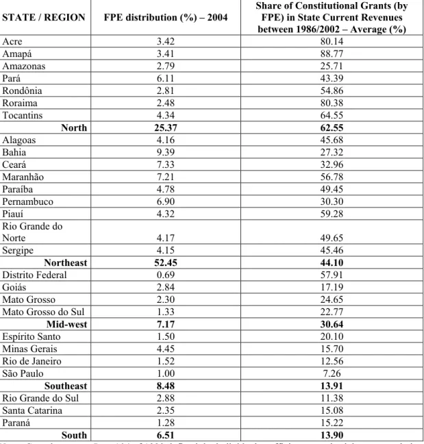
Table 4 in the Annex shows the results of the distribution of the ‘FPE’ between states/regions for the year, 2004, as determined by Complementary Law 62 of 1989, and the average participation (in %) of transfers via the ‘FPE’ in the current revenue of states.11

Analyzing these data, it is possible to notice that there are two regions which are net receivers and two net contributors of resources in Brazil. The North and Northeast are net receivers and the Southeast and South are net contributors.12 It is also possible to see that the regions that are net contributors are the ones that are less dependent on transfers in their current revenue.

A criticism that needs to be pointed out is that the Brazilian system of vertical transfers aims to correct equity matters between regions, but does not consider efficiency controls. As a consequence, it is possible to allocate these funds in a way that does not necessarily coincide with the best interests of society. This will be explored in the following sections.

4. Wage expenditure in state governments

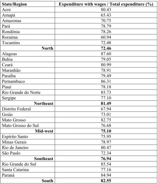
The participation of expenditures on wages in the total expenditure of the states and regions, does not, at first sight, reveal the preference of the bureaucracy in the poorer states for higher wages, when compared with the richer states, as is shown in table 5 in the Annex.

In all states and regions, the share of expenses with wages in total expenditure is over 70%. However, analyzing the capacity of the bureaucracy to generate premium wages for the public sector, when compared to the private sector in the same states, it is possible to have a clearer picture of the allocation choice of the bureaucracy. This is to be explored next.

10_{The IPI is a tax on consumption charged in the state of origin on the value added at each stage of the} production chain.

11_{These data are available on the website of the National Treasury of Brazil.}

12_{We did not classify the Mid-west region due to the Federal District, because it receives funds to pay the} wages of public servants. If it is disregarded, the region certainly would be a net receiver.

(6)

To analyze the wages paid in the state public sector and to test if there is a premium or penalty in relation to the wages paid in the private sector, we use the methodology proposed by Oaxaca (1973). The essence of this methodology is to decompose the wages into the observable and non-observable characteristics of the workers. For the calculation of the wage differentials, we used data from the 26 Brazilian states and the Federal District from 1995 to 2004. Our primary data source was the National Survey by Household Sample (PNAD), published by the Brazilian Institute for Geography and Statistics (IBGE).13 For calculation of the wage differentials we only included employed people, between 18 and 65 years old, working in urban areas, excluding domestic workers and employers. These selections in the general sample were necessary in order to make public and private workers comparable14. Information that did not allow us to identify if the worker was in the public or private sector was also disregarded. Only data relating to the primary job were considered, since secondary occupations have specific characteristics that could alter the results. Finally, all individual wages were adjusted to a 40-hour working week. 15

In order to use the technique developed by Oaxaca (1973), the following observable characteristics of the workers were chosen: gender, color, age, square of the age, educational level in years of study, square of years of study, years experience in the job, square of the years of experience and participation in unions.16

In order to look for robustness in the results, additional tests were made considering different samples of private sector workers.

For public workers, we used a sample considering statutory public workers17 and CLT public workers18. For the private workers we used three distinct samples: one considering employees in the manufacturing sector, another considering employees in the formal private sector (workers with rights in accordance with Law 5452 of May, 1943) and a last one considering all employees (formal and informal workers). Initially we were not going to use the manufacturing sector, but Van Rijckeghem and Weder (1997)19 used this sector to study wage differentials, because it is closer to the public sector in terms of activities, especially at lower wage levels. The separation of private workers into formal and informal was used to parallel the methodology used by Panizza (2001). The descriptive statistics of the variables used in each sample are included in Appendix 1.

13_{We adopted this period because of our aim of carrying out a comparative analysis in an environment where} the states were under severe budgetary constraint after 1995 .The year 2000 could have been included but this is a Census year , and PNAD and CENSUS are not run in the same years and are not directly comparable. 14_{Self-employed workers in the public sector do not exist (as they do in the private sector) and the entrance} tests and simplified selection processes impose a minimum age of 18 as an admission requirement. In addition, civil servants rarely works in rural areas, except in specific isolated cases, such as border or agricultural inspections.

15_{There is an implicit assumption in this calculation, namely that the value of the hourly wage does not vary} according to the number of hours worked, and that the majority of employees work 40 hours a week.

16_{The performance of the union of one specific category can result in the establishment of higher wages than} those defined in a competitive equilibrium situation.

17_{Statutory workers are civil servants who have legally guaranteed job tenure and they receive full pensions} (100% of last wage) when they retire.

18_{CLT public workers are public workers contracted with the same rules as formal workers in the private} sector. They do not have the legal right of job tenure, but, nonetheless, it is difficult to fire them. We could say that their job tenure is more precarious than that of statutory workers.The expression CLT has its origin in Law 5452 of May of 1943, entitled the Consolidation of Labor Laws (CLT in Portuguese).

(7)

The results found for the public workers sample20 in comparison to private workers can be seen in table 6 in the Annex:

It is possible to observe from the results that the wage premium for state public workers in Brazil is not uniform across the different regions. In the Northern states the premium is the highest. In the richest region in the country, the Southeast, the premium less significant, around 7%.

Based on this data it is possible to affirm that there is a dichotomy in the relationship between the wages of the public and the private sectors in the states/regions. The issue to be analyzed - and this is at the heart of this paper - is to identify if this difference is influenced by the system of vertical transfers. The next section presents the empirical analysis.

5. Empirical analysis 5.1. The Model

The specification used to verify the appropriation of resources by the bureaucracy was the following:21

it i it it

it

it GRANTS ELECTION PUBLICWORKERS f

Y =_β0 +_β1 +_β2 ₋1+_β3 + +_ε [1]

where i = 1, 2....,.27 states, t = 1995, 1996...2004, f is the individual effect and_i

it

ε is the random error term. Our sample consists of 26 Brazilian states and the Federal District, between the years 1995 and 2004.

The estimates are calculated using unbalanced panel techniques, since not all variables have complete series. The technique used was the Least Squares Dummy Variable Model (LSDV).

Y represents the wage differential between the public and the private sectors.

GRANTS is the percentage of transfers of the federal government on current state

revenues. The importance of the transfers in sub-national governments as a revenue source, even if ambiguous in its effect on the size of government, can be observed in studies by Oates (1985, 1989), Zax (1989), Bevilacqua (2002), Stein (1999), and Seitz (2000). The data source is the National Treasury. We expect the associated variable coefficient to be positive. The higher the volume of resources from transfers, the greater the incentive for the bureaucracy to appropriate the available resources, via wage premiums. ELECTION is a dummy with value 1 for the years of election and zero otherwise. The data source for construction of this variable was the Superior Electoral Superior. Works by Alesina, Roubini and Cohen (1997), Blais and Nadeau (1992), Cossio (2001), among others, have pointed out the influence of the political cycle on fiscal results. We made some initial tests and the best choice was the ELECTIONvariable lagged 1 period.

ERS

PUBLICWORK is the number of public workers as a percentage of the total

workers of the state. Given the considerable participation of public jobs in Brazilian states, we considered the use of this variable as a control. It was expected that the participation of

20_{The basic statistics of the variables adopted to calculate the wage differentials using the technique of} Oaxaca (1973) can be found in Appendix 2.

21_{The basic statistics of the variables adopted are in Appendix 2 (two last lines: GRANTS and}

(8)

public workers would reduce the existing wage differential, since the budget constraint imposes limits to keeping this difference.

To control for possible differences among regions, we use dummy variables for each of them, not reported in the estimates. These differences, for example, the cultural factors of each region, urbanization and industrialization, even if difficult to measure must be considered in the regression estimates in order to avoid bias.22 To control a time differences, we use dummy variables for each year.

Inflation rate, rate of unemployment and per capita GDP were not included as controls. Inflation rate and rate of unemployment data are available only for some state capitals.23 As the formula for the calculation of the ‘FPE’ distribution considers the per capita GDP, we choose not to include this variable.

All the estimates presented heteroskedasticity and in some cases auto-correlation. Estimates were run as a control for these problems. The descriptive statistics of the variables used are included in Appendix 2.

5.2. Primary results

The results of the estimates of the equation [1] can be seen in table 7 in the Annex. For each sample we present two columns. The first column includes the general results from the model and the second shows the significant variables under the 10% level of significance only. The control variables did not show a significance pattern among the different samples. In the first estimate [1], no control variable is significant. In the second estimate [2], the ELECTION has a 1% level of significance and its signal shows that there is an increase in the wage differential in the year subsequent to the election. In the third estimate [3], the PUBLICWORKERS was significant in the first column, but it was not in second. The estimated signal of this variable was negative, as we expected. A larger participation of public workers in the total of employees, given the existence of a budgetary constraint, reduces the wage differential because the amount of resources available for wage increases will be smaller.

Anyway, the most important variable of our tests (the aim of this study is to analyze the relationship between grants and wage differentials), GRANTS, exhibits the same results. The increase in the share of transfers in the states’ current revenue raised the wage differential between the public sector and the private sector in every related sample in the table. The results proved how highly significant this was and what a strong influence they had on results (see their coefficients in the table).

5.3. Robustness and sensitivity of the coefficients.

In order to analyze if the basic results are sensitive to the results of a specific state, a concentrated group of states, or some specific group in the public sector in the states (outliers), we will carry out some additional tests.

22_{Such an individual effect tries to capture the impact that the non-observable heterogeneity exerts on the} dependent variable.

23_{Inflation and/or unemployment rates are used in the estimates in panel for countries. See Tavares (2002),} Volkerink and Haan (2001) and Perotti and Kontopoulos (2002).

(9)

Individual effect or in groups of states.

In the first estimate [1], the states of Acre, Amapá and Roraima are “outliers” of sample. 24 In the second estimate [2], the states of Acre and Amapá influenced too the results of the estimates.25 Finally, in the third sample, the states of Acre, Amapá, Maranhão, Pernambuco and Rio Grande do Norte had exerted the same kind of influence. 26_Starting from the available data, we obtained a new estimate with the same technical procedure for each sample, in which we excluded those states that had exerted an influence on the group as a whole. Although we did not get to understand the individual or group effect for those states, we show the results in table 8 in the Annex.

All results, in general, presented similar levels of significance, magnitude and signal when compared to the coefficients obtained previously. The exception was the variable ELECTION in the first estimate (table 7). It became significant at the level of 1% in the first and second estimates (table 8). Once again, we found strong and robust results in the variable GRANTS . So, even when we excluded the states that could be influencing the different samples (outliers), the increase of the share of transfers in the current revenue of the states increased the wage differential between the public and private sector.

6. Main results

The Brazilian grants system is designed to reduce the economic and social inequalities between the states. It is carried out by the federal government and transfers resources from the richer states (states from the Southeastern and Southern regions) to the poorer states (from the North, Northeast and Mid-west regions of the country). However, these transfers occur without control over the efficiency of the expenditure and state governments have a lot of freedom and flexibility in deciding how to allocate the transferred resources.

In order to analyze the relationship between the allocation of these resources and the wage level of public servants, we developed indicators for wage differentials between the public and private sector for each Brazilian state government. The results show the existence of elevated premiums (positive differentials) in the wages paid to state bureaucrats in the North, Northeastern and Mid-west regions of the country, unlike the numbers for the Southern and Southeastern regions, which report negative or close to zero differentials (penalty) in the wages paid to state government bureaucrats.

The empirical tests demonstrated that the grant system, which transfers resources from the federal government to the states, is one of the main causes of the existence of high wage differentials in some regions of the country. The significant and positive (consequently, robust) results for all samples indicated that a share of these resources (arising from the transfers) is being siphoned off by the state bureaucracy via wage premiums. The hypothesis tests demonstrated that there is no significant difference between

24_{The procedure of the Chow Predictive Test defined the following states: Acre (F = 1.74 and p-value =} 0.08), Amapá (F = 1.66 and p-value = 0.10), and Roraima (F = 128.94 and p-value = 0.00).

25_{Acre (F = 2.60 and p-value = 0.04) and Amapá (F = 7.15 and p-value = 0.00).}

26_{Acre (F = 3.81 and p-value = 0.07), Amapá (F = 6.04 and p-value = 0.03), Maranhão (F=2.29 and p-value =} 0.02), Pernambuco (F = 2.44 and p-value = 0.01) and Rio Grande do Norte (F = 1.87 and p-value = 0.06).

(10)

the coefficients that result from the application of our model to different samples and sub-samples and, consequently, they make it possible for us to make generalized arguments, which indicates the robustness of the results obtained in our study.

Another important result from our tests is the influence of the political cycle on the increase in the positive wage differentials for public employees, which corroborates the arguments presented in others studies on this subject, such as those in Alesina, Roubini and Cohen (1997). The positive and significant coefficient of the variable ELECTION (t+1) caught the effect of the electoral year, namely, the incentive to increase the positive wage differentials for the state bureaucracy in periods close to elections in order to achieve greater approval ratings and, consequently, to get re-elected, or to get one’s political successor elected. Consequently, we realize that there is a siphoning off of resources coming from the inter-governmental transfers by the state bureaucracy, which aims to maintain (or create) privileges for themselves, by paying wage premiums, as represented by the positive wage differentials between public and private employees.

The non-significance of the variable PUBLICWORKERS can be explained by the severe budgetary restrictions that state governments had to face up to after introduction of the Real Plan in 1995, because it imposed limits on the hiring of new civil servants and on wage increases, in a purely discretional way.

REFERENCES

Alesina, A., Roubini, N. and Cohen, G. Political Cycles and the Macroeconomy. Cambridge: MIT Press, 1997.

Amihud, Y.; Lev, B. (1981) Risk reduction as a managerial for conglomerate mergers. Bell

Journal of Economics 12:605-617.

Bacha, E. (1994) O fisco e a inflação: uma interpretação do caso brasileiro. Revista de

Economia Política, v.14, n.1,p. 53, jan./mar.

Becker, G.; Stigler, J. (1974) Law Enforcement, Malfeasance, and the Compensation of Enforces, Journal of Legal Studies, vol V, pp1-19.

Bevilacqua, A.S. (2002) State Government Bailouts in Brazil. Working paper of

Inter-American Development Bank.

Bendor J., Taylor, S. and van Gaalen, R. (1985) Bureaucracy expertise versus Legislative Authority: A model of deception and monitoring in budgeting. American Political

Science Review 79, pp 1041-60.

Blais, A.; Dion, S. (1991) The budget-maximizing bureaucrat: Appraisals and evidence. Pittsburgh, PA.: University of Pittisburgh Press.

Blais, A., Nadeau, R. (1992) The electoral budget cycle. Public Choice, Volume 74, number 4.

Boardman, A.E.; Vining,A.R. (1989) Ownership and Performance in competitive environments: a comparison of the performance private, mixed and state-owed enterprises. Journal of Law and Economics 32(1), pp: 1-39.

Boardman,A.E. Vining,A.R. (1992) Ownership versus competition: efficiency in Public Enterprise. Public Choice 73, pp: 205-39.

Borjas, G.J. (1980) Wage determination in the Federal Government: The Role of Constituents and Bureaucrats. The Journal of Political Economy, Vol. 88, No.6.

(11)

Breton, A.; Wintrobe, R. (1975) The equilibrium Size of a Budget Maximizing Bureau.

Journal of Political Economy 83, pp: 195-207.

Casas-Pardo, J.; Puchades-Navarro,M. (2001) A critical comment on Niskanen´s model.

Public Choice 107:147-167.

Cossio, F. A. B. (2001). O comportamento fiscal dos governos estaduais brasileiros: determinantes políticos e efeitos sobre o bem estar dos seus estados e seus. Prêmio

Tesouro Nacional.

Downs, A. (1967) Inside of Bureaucracy. Boston: Little Brown.

Fisher, I.W.; Haal, G.R. (1969) Risk and corporate rates of return. Quarterly Journal of

Economics 83:79-92.

Greene, W. H. (1997) Econometric Analysis. Third Edition. Prentice Hall. Upper Saddle River, NJ.

Grossman, P.J. (1990) The impact of federal and states grants on local government spending: a test of the fiscal illusion hypothesis. Public Finance Quarterly 18(3):313-327.

Gugler, K. (1998) Corporate Owership Structure in Austria. Empirica 25(3), pp:285-307. Hayes, K., Razzolini, L. and Ross, L.B. (1998) . Bureaucratic choice and non-optimal

provision of public goods: theory and evidence. Public Choice 33:1-20. Hamilton, L. C. (2004). Statistics with Stata. Ed. Books Cole - Thomson

Johnson, B.T.; Libecap, G.D. (1989). Contracting problems and regulation: the case of the fishery. American Economic Review, 72, 1005-22.

Koenker, R.; Basset,G. (1978). Regression Quantilies. Econometrica 46(3):33-50.

Kraay, R.; Van Rijckeghem C. (1995) Employment and wages in Public sector: a cross sector srtudy. IMF Working Paper.

Moesen, W.; Van Cauwenberge.P. (2000). The status of the budget constraint, federalism and relative size of government: a bureaucracy approach. Public Choice 104: 207-224.

Migué, J.; Bélanger,G. (1974) Toward a general theory of managerial discretion. Public

Choice, 17,27-43.

Miller, G.J.; Moe, T.M. (1983) Bureaucrats, Legislators, and size of Government. American

Polilical Science 77, pp: 297-322.

Niskanen, W.A. (1971) Bureaucracy and representative government, Chicago:Aldine-Atherton.

Oates, W.E. (1985), Searching for Leviathan: An Empirical Study, American Economic

Review 75,748-757.

Oates, W.E. (1989). Searching for Leviathan: A reply and some further reflections.

American Economic Review 79: 578-83.

Oaxaca, R. (1973). Male-female wage differentials in urban labour markets. International

Economic Review, 140, 693-709.

Panizza, U. (2001) Public Sector wages and Bureaucratic quality: evidence from Latin American, Economia, Fall.

Peltzman, S. (1976) Toward a more general theory of regulation. Journal of Law and

Economics. 23,209-87.

Perotti, R. and Kontopoulus,Y. (2002). Fragmented Fiscal Policy. Journal of Public

(12)

Seitz, H. (2000) Fiscal Policy, Deficits and Politics of Subnational Governments: The Case of the German Laender. Public Choice, volume 102, number 3 - 4.

Stein, E. (1999). Fiscal decentralization and Government size in Latin America. Journal of

Applied Economics. Vol II, no 2, 357-391.

Stigler,G. J. (1971) The theory of economic regulation. Bell Journal of Economics and

Management Science, 2,3-21.

Tullock, G. (1965) The politics of Bureaucracy, Washington, D.C: Public Affairs Press. Van Rijckeghem, C.; Weder, B. (1997). Corruption and rate of temptation: do low

wages in the civil service cause corruption? IMF Working Paper 97/73.

Volkerink, B.; de Haan, J. (2001). Fragmented Government Effects on Fiscal Policy: New Evidence. Public Choice, Volume 109: 221-242.

Worthington, A.; Dollery, B. E. (1998) The political determination of intergovernmental grants in Austrália. Public Choice Volume 94:299-315.

Zax, J.S. (1989) Is there a Leviathan in your neighborhood? The American Economic

Review, Volume 79, number 3, 560-567.

ANNEX

Table 1: The share (%) of discretionary grants in the current revenue of states in the period 1986-2002.

STATES AVERAGE STATES AVERAGE

Acre 0.11 Paraíba 0.06

Alagoas 0.02 Paraná 0.05

Amapá 0.23 Pernambuco 0.05

Amazonas 0.02 Piauí 0.08

Bahia 0.07 Rio de Janeiro 0.03

Ceará 0.03 Rio Grande do Norte 0.06

Distrito Federal 0.19 Rio Grande do Sul 0.03

Espírito Santo 0.07 Rondônia 0.07

Goiás 0.05 Roraima 0.17

Maranhão 0.06 Santa Catarina 0.04

Mato Grosso 0.07 São Paulo 0.01

Mato Grosso do Sul 0.09 Sergipe 0.04

Minas Gerais 0.04 Tocantins 0.05

Pará 0.13 Brazil 0.07

(13)

Table 2: Taxes that form the State Participation Fund (FPE) STATES/REGIONS

Average participation of state/region industrialized products tax (IPI) in country’s total. Data from 1994 to 2002

(%)

Average participation of state/region income tax in country’s total. Data from 1994

to 2002 (%) Acre 0.01 0.04 Amapá 0.03 0.13 Amazonas 0.62 0.61 Pará 0.34 0.58 Rondônia 0.05 0.13 Roraima 0.02 0.03 Tocantins 0.04 0.03 North 1.14 1.58 Alagoas 0.25 0.22 Bahia 3.07 1.78 Ceará 0.87 1.00 Maranhão 0.52 0.24 Paraíba 1.76 0.30 Pernambuco 0.27 1.20 Piauí 0.34 0.19

Rio Grande do Norte 0.29 0.28

Sergipe 0.27 0.23

Northeast 7.68 5.49

Distrito Federal 0.60 10.62

Goiás 0.95 0.74

Mato Grosso 0.13 0.28

Mato Grosso do Sul 0.34 0.30

Mid-west 2.03 11.95 Espírito Santo 4.42 0.91 Minas Gerais 8.93 4.90 Rio de Janeiro 9.01 17.61 São Paulo 51.80 47.82 Southeast 74.17 71.25

Rio Grande do Sul 5.44 3.64

Santa Catarina 6.77 4.42

Paraná 2.73 1.64

South 14.95 9.71

Note: Revenue tax and Industrialized Products tax data from www.receita.fazenda.gov.br

Table 3: Average participation of the regional GDP in Brazil’s GDP – 1985 to 2003 , highlighting the state of São Paulo.

REGIONS Participation of the regional GDP in Brazil’s GDP (%)

Mid-west 6.84 North 4.72 Northeast 13.24 South 17.89 Southeast 57.30 São Paulo 33.88

(14)

Table 4: Distribution of the resources of State Participation Fund (FPE) and the average participation of the Grants in Current Revenues

STATE / REGION FPE distribution (%) – 2004 Share of Constitutional Grants (byFPE) in State Current Revenues between 1986/2002 – Average (%) Acre 3.42 80.14 Amapá 3.41 88.77 Amazonas 2.79 25.71 Pará 6.11 43.39 Rondônia 2.81 54.86 Roraima 2.48 80.38 Tocantins 4.34 64.55 North 25.37 62.55 Alagoas 4.16 45.68 Bahia 9.39 27.32 Ceará 7.33 32.96 Maranhão 7.21 56.78 Paraíba 4.78 49.45 Pernambuco 6.90 30.30 Piauí 4.32 59.28 Rio Grande do Norte 4.17 49.65 Sergipe 4.15 45.46 Northeast 52.45 44.10 Distrito Federal 0.69 57.91 Goiás 2.84 17.19 Mato Grosso 2.30 24.65

Mato Grosso do Sul 1.33 22.77

Mid-west 7.17 30.64 Espírito Santo 1.50 20.10 Minas Gerais 4.45 15.70 Rio de Janeiro 1.52 12.56 São Paulo 1.00 7.26 Southeast 8.48 13.91

Rio Grande do Sul 2.88 11.38

Santa Catarina 2.35 15.08

Paraná 1.28 15.22

South 6.51 13.90

Note: Complementary Law 104 of 1989 defined the individual coefficients: territorial area, population

and the inverse of the per capita income of each state. The source of the coefficients is the Secretariat of the Treasury (2004). The average of the constitutional transfers was calculated from data available in IPEADATA.

(15)

Table 5: Average of expenses with wages in the Total Expenditure in Brazilian states from 1985/1994

State/Region Expenditure with wages / Total expenditure (%)

Acre 80.43 Amapá 65.43 Amazonas 70.75 Pará 78.79 Rondônia 78.26 Roraima 60.94 Tocantins 72.48 North 72.46 Alagoas 87.60 Bahia 79.05 Ceará 80.99 Maranhão 78.91 Paraíba 79.49 Pernambuco 86.31 Piauí 78.18

Rio Grande do Norte 85.73

Sergipe 77.10

Northeast 81.49

Distrito Federal 67.94

Goiás 73.01

Mato Grosso 82.75

Mato Grosso do Sul 76.68

Mid-west 75.10 Espírito Santo 75.95 Minas Gerais 78.97 Rio de Janeiro 80.47 São Paulo 72.34 Southeast 76.94

Rio Grande do Sul 85.54

Santa Catarina 77.16

Paraná 84.94

South 82.55

Source: IPEADATA

Table 6: Premium or penalty in the average wages of employees for Brazilian Region (average 1995-2004) Regions [1] [2] [3] North 57.4% 18.9% 21.2% Northeast 5.7% 8.4% 15.2% Mid-west 13.8% 9.0% 14.3% Southeast 3.2% 6.2% 7.5% South -3.2% 2.2% 1.2% Brazil 17.3% 9.8% 13.6%

Note: [1] Statutory + CLT public workers / Manufacturing private sector workers; [2] Statutory + CLT public

workers / Private Formal Sector; [3] Statutory + CLT public workers / All Private Sector (Formal and Informal Workers).

(16)

Table 7: Grant effects on wage differentials between the public and private sector. [1] [2] [3] GRANTS -0.471 0.325 0.365 0.323 0.378 (-0.66 ) ( 2.34 )** ( 4.46)*** (2.57)*** (5.00)*** ELECTION+1 0.707 0.732 0.275 0.276 0.310 0.311 (3.28 )*** (3.12)*** (6.06 )*** (6.04 )*** (7.13)*** (7.12)*** PUBLIC WORKER 3.191 2.647 0.078 0.106 (2.08)** ( 2.69)*** (0.40) (0.58) CONSTANT -0.713 -0.744 -0.151 -0.140 -0.139 -0.124 ( -2.14)** (-2.04)** (-2.79 )*** ( -2.99 )*** (-2.71)*** (-2.83)*** Observations 243 243 243 243 243 243 Number of groups 27 27 27 27 27 27 R2 _0.196 _0.194 _0.322 _0.322 _0.398 _0.397 Z statistics in parentheses

* significant at 10%, ** significant at 5%, *** significant at 1%

Note: [1] Considering the wage differential between Statutory + CLT public workers / Manufacturing

private sector workers; [2] Considering the wage differential between Statutory + CLT public workers / Private Formal Sector; [3] Considering the wage differential between Statutory + CLT public workers / All Private Sector (Formal and Informal Workers).

(17)

Table 8: Grant effect on the wage differential between the public and private sector, excluding the outliers (states) [1] [2] [3] GRANTS 0.338 0.385 0.278 0.316 0.226 0.335 (1.79 )* (3.08)*** (2.25)** ( 4.05)*** (2.22)** (4.90)*** ELECTION+1 0.267 0.265 0.233 0.233 0.278 0.279 (4.58 )*** (4.56)*** (5.68)*** (5.68)*** (7.59)*** (7.56)*** PUBLIC WORKER 0.103 0.070 0.202 ( 0.37) (0.39) (1.31) CONSTANT -0.121 -0.114 -0.104 -0.110 -0.080 ( -1.51) (-2.28)** (-2.38)** ( -2.44)** (-2.04)** Observations 216 216 225 225 198 198 Number of groups 24 24 25 25 22 22 R2 0.223 0.223 0.300 0.299 0.500 0.495 Z statistics in parentheses

[1] [2] [3] GRANTS 0.338 0.385 0.278 0.316 0.226 0.335 (1.79 )* (3.08)*** (2.25)** ( 4.05)*** (2.22)** (4.90)*** ELECTION-1 0.267 0.265 0.233 0.233 0.278 0.279 (4.58 )*** (4.56)*** (5.68)*** (5.68)*** (7.59)*** (7.56)*** PUBLIC WORKER 0.103 0.070 0.202 ( 0.37) (0.39) (1.31) CONSTANT -0.121 -0.114 -0.104 -0.110 -0.080 ( -1.51) (-2.28)** (-2.38)** ( -2.44)** (-2.04)** Observations 216 216 225 225 198 198 Number of groups 24 24 25 25 22 22 R2 _0.223 _0.223 _0.300 _0.299 _0.500 _0.495 Z statistics in parentheses

Note: [1] Considering the wage differential between Statutory + CLT public workers / Manufacturing private

sector workers; [2] Considering the wage differential between Statutory + CLT public workers / Private Formal Sector; [3] Considering the wage differential between Statutory + CLT public workers / All Private Sector (Formal and Informal Workers).

(18)

Table 9: Grant effect on the wage differential between the public and private sector, calculated for the sub-sample of the lowest 10 % of wages.

[1] [2] [3] GRANTS 0.445 0.517 0.8098 0.483 0.335 (2.13)** (3.40)*** (5.11)*** (3.97)*** (3.10)*** ELECTION-1 0.061 0.2065 0.053 (0.77) (3.11)*** (1.11) PUBLIC WORKER 0.4056 -0.7844 -0.27 (0.95) (-2.12)*** (-1.25) CONSTANT 0.048 0.093 0.0937 0.113 0.085 (0.78) (1.36) (1.77)* (2.71)*** (1.78)* Observations 134 135 134 134 135 Number of groups 27 27 27 27 27 R2 _0.270 _0.239 _0.340 _0.255 _0.193 Z statistics in parentheses

Note: [1] Considering the wage differentials between Statutory + CLT public workers / Manufacturing

private sector workers; [2] Considering the wage differentials between Statutory + CLT public workers / Private Formal Sector; [3] Considering the wage differentials between Statutory + CLT public workers / All Private Sector (Formal and Informal Workers).

Table 10: Grant effect on the wage differential between the public and private sector, calculated for the sub-sample of median wages.

[1] [2] [3] GRANTS 0.604 0.428 0.568 0.479 0.521 0.490 (3.43)*** (3.09)*** (5.02)*** (5.20)*** (5.93)*** (5.37)*** ELECTION-1 0.130 0.045 0.107 0.064 0.034 (2.08)*** (0.90) (2.33)*** (1.72)*** (0.93) PUBLIC WORKER -0.5759 -0.2931 -0.2820 -0.2968 (-1.63) (-1.21) (-1.66)* (-1.55) CONSTANT -0.030 -0.035 -0.039 -0.041 -0.014 -0.012 (-0.72) (-0.83) (-1.11) (-1.18) (-0.52) (-0.33) Observations 134 134 134 134 134 135 Number of groups 27 27 27 27 27 27 R2 _0.277 _0.247 _0.364 _0.352 _0.401 _0.363 Z statistics in parentheses

Note: [1] Considering the wage differential between Statutory + CLT public workers / Manufacturing

private sector workers; [2] Considering the wage differential between Statutory + CLT public workers / Private Formal Sector; [3] Considering the wage differential between Statutory + CLT public workers / All Private Sector (Formal and Informal Workers).

(19)

Table 11: Grant effect on the wage differential between the public and private sector calculated for the sub-sample of the highest 10% of wages

[1] [2] [3] GRANTS 0.544 0.312 0.250 0.168 0.426 0.271 (2.48)** (1.97)** (2.25)** (1.84)* (4.32)*** (3.14)*** ELECTION-1 0.048 0.104 0.065 0.053 (0.62) (2.22)** (1.66)* (1.24) PUBLIC WORKER -0.5559 -0.2689 -0.3531 (-1.2) (-1.14) (-1.60) CONSTANT -0.022 0.039 -0.079 -0.082 -0.066 -0.050 (-0.46) (0.62) (-2.64)*** (-2.73)*** (-2.26)** (-1.37) Observations 134 135 134 134 134 135 Number of groups 27 27 27 27 27 27 R2 _0.203 _0.148 _0.143 _0.131 _0.240 _0.175 Z statistics in parentheses

Note: [1] Considering the wage differentials between Statutory + CLT public workers / Manufacturing

private sector workers; [2] Considering the wage differentials between Statutory + CLT public workers / Private Formal Sector; [3] Considering the wage differentials between Statutory + CLT public workers / All Private Sector (Formal and Informal Workers).

APPENDIX 1

A.1.1 Table: Variables adopted in the calculation of the wages of the employees in the private manufacturing sector

Variables Average Std. Err Minimum Maximum

Dependent variable LN adjusted wage 1.97 0.81 -1.74 6.43 Independent variable Years of study 7.31 3.95 1 16 Years of study2 _69.11 _65.24 ₁ ₂₅₆ Age 33.19 10.92 18 98 Age2 _1221.14 _827.33 ₃₂₄ ₉₆₀₄ Gender Dummy 0.79 0.40 0 1 Race Dummy 0.54 0.49 0 1

Years of experience (in job) 4.62 6.18 0 65

Years of experience (in job)2 _59.65 _151.62 ₀ ₄₂₂₅

(20)

A.1.2 Table: Variables adopted in the calculation of the wages of employees in the formal private sector

Years of experience (in job) 2 _61.55 _147.01 ₀ ₄₂₂₅

Union Dummy 0.27 0.44 0 1

A.1.3 Table: Variables adopted in the calculation of the wages of employees in the formal and informal private sector

Years of experience (in job)2 _57.18 _144.67 ₀ ₄₂₂₅

Union Dummy 0.23 0.42 0 1

A.1.4 Table: Variables adopted in the calculation of the wages of statutory public employees and CLT public employees.

Dependent variable LN adjusted wage 2.64 0.82 -1.56 6.90 Independent variable Years of study 12.10 3.70 1 16 Years of study2 _160.29 _78.50837 ₁ ₂₅₆ Age 38.94 9.78 18 96 Age2 _1612.75 _807.43 ₃₂₄ ₉₂₁₆ Gender Dummy 0.41 0.49 0 1 Race Dummy 0.57 0.49 0 1