Demand, Supply and Markup Fluctuations

Demand, Supply and

Markup Fluctuations

Carlos Santos

Luís F. Costa

Paulo Brito

Working Paper

# 609

2016

Demand, Supply and Markup Fluctuations

Carlos Santos

, Luís F. Costa

and Paulo Brito

13.10.2016

Abstract

The cyclical behavior of markups is at the center of macroeconomic de-bate on the origins of business-cycle ‡uctuations and policy e¤ectiveness. In theory, markups may ‡uctuate endogenously with the business cycle due to sluggish price adjustment or to deeper motives a¤ecting the price-elasticity of demand faced by individual producers. In this article we make use of a large …rm- and product-level panel of Portuguese manufacturing …rms in the 2004-2010 period. The biggest empirical challenge is to separate supply (TFP) from demand shocks. Our dataset allows to do so, by containing

Financial support by FCT (Fundação para a Ciência e a Tecnologia), Portugal, is grate-fully acknowledged. This article is part of the Strategic Project (UID/ECO/00436/2013), under the project Ref. UID/ECO/00124/2013 and by POR Lisboa under the project LISBOA-01-0145-FEDER-007722. Carlos Santos gratefully acknowledges FCT research fellowship CONT-DOUT/114/UECE/436/10692/1/2008 under the programme Ciência 2008. We would like to thank Vasco Matias and André Silva for their research assistance, and INE (Statistics Portugal), especially So…a Pacheco, M. Arminda Costa, and Carlos Coimbra, for their help with micro-data. Comments and suggestions by How Dixon, Huiyu Li and by the participants at the 11th World Congress of the Econometric Society (Montréal), 30th Annual Congress of the European Economic Association (Mannheim), 8th Meeting of the Portuguese Economic Journal (Braga) and at at seminars in EIEF (Rome) and ISEG of ULisboa (Lisbon) are gratefully acknowledged. The usual disclaimer applies.

y_{Nova School of Business and Economics, UNL, 1099-032 Lisboa, Portugal.}

information on product-level prices at a yearly frequency. Furthermore, markups are mismeasured when calculated with the labor share. We use the share of intermediate inputs instead. Our main results suggest that markups are pro-cyclical with TFP shocks and generally counter-cyclical with demand shocks. We also show how markups become procyclical if the markup is obtained using the labour share instead of intermediate inputs. Adjustment costs create a wedge between the labour share and the actual markup which explain the observed correlations.

Keywords: Markups, Demand Shocks, TFP shocks JEL classification: C23, E32, L16, L22

1

Introduction

The cyclical behavior of markups, i.e. the wedge between prices and marginal costs, has been at the center of macroeconomic debate on the origins of business-cycle ‡uctuations and policy e¤ectiveness. For instance, when analyzing the role of varying markups in …scal-policy e¤ectiveness, Hall [2009] refers: "models that deliver higher multipliers feature a decline in the markup ratio of price over cost

when output rises (...)".1

In theory, markups may ‡uctuate endogenously with the business cycle due to sluggish price adjustment (undesired endogenous markups) or to deeper motives a¤ecting the price-elasticity of demand faced by individual producers (desired endogenous markups). The undesired type is present in macroeconomic models that assume sticky prices as state-dependent models of the menu-costs sort, e.g. Mankiw [1985], and time-dependent models as Calvo [1983], Rotemberg [1982]

or the sticky-information model of Mankiw and Reis [2002]. The undesired type comprises a large number of reasons including more general preferences outside the CES benchmark as in Bilbiie et al. [2012], Feenstra [2003] or Ravn et al. [2008], heterogeneity of demand as in Galí [1994] or Edmond and Veldkamp [2009],

intra-industrial competition2 _{as in Barro and Tenreyro [2006], Costa [2004] or}

Rotemberg and Woodford [1991], feedback e¤ects as in Jaimovich [2007], amongst other motives. For a survey see Rotemberg and Woodford [1999]. de Loecker et al. [2016] use a similar methodology to the one followed in this article, to study the e¤ect of trade liberalization on prices and markups of companies in India. They …nd evidence of increasing markups after trade liberalization due to the limited pass-through of cost savings into prices. This limits the gains from trade, at least in the short run.

The empirical evidence is mixed. Rotemberg and Woodford [1999] use the evi-dence on the cyclical behavior of the labor share in total income, a macroeconomic approach, to conclude that average markups are unconditionally counter-cyclical, so they have to be counter-cyclical with demand shocks. Martins and Scarpetta [2002] use a di¤erent approach, closer to Industrial Organization (IO), but reach similar conclusions for a sample of industries in G5 countries. More recently, Juessen and Linnemann [2012] provide evidence of counter-cyclical markups for a panel of 19 OECD countries; Afonso and Costa [2013] …nd that markups are counter-cyclical with …scal shocks for 6 out of 14 OECD countries and pro-cyclical for 4 of them; Nekarda and Ramey [2013] …nd either acyclic or pro-pro-cyclical markups with demand shocks for US industries.

The inconclusive results may be related with the fact that separating demand

and supply shocks is a di¢ cult task in the absence of separate price and quantity data. Thus, if the supply and demand shocks have di¤erent cyclicality, a "weighted average" of the two may exhibit either pro- or counter-cyclical behavior, depending on which shock is more prevalent. Furthermore, most articles use the labor share to obtain the markups. Labor is subject to adjustment cost, which create a wedge between the markup and the labor share.

Three empirical challenges are at the origin of the inconclusive results: (i) us-ing revenues instead of quantities, results in productivity measures contaminated with demand shocks in imperfectly competitive markets, as noticed by Klette and Griliches [1996]; (ii) estimating total factor productivity (TFP) is usually poised by the input-endogeneity problem in production functions that has been identi…ed since at least Marschak and Andrews [1944]; and (iii) using labor (and its share) as the ‡exible input that proxies marginal-cost ‡uctuations is problematic in the

presence of labor-market frictions3. We overcome problem (i) by using

meaning-ful quantities for single-product …rms in the estimation of production and cost functions and overcome problem (ii) by extending recent results to address the endogeneity problem for input utilization - see Olley and Pakes [1996], de Loecker [2011] and Gandhi et al. [2013]. In particular, we show that there is no mul-ticollinearity problem (Ackerberg et al. [2006], Bond and Soderbom [2005] and Gandhi et al. [2013]) when …rm level prices are observed and demand shocks are persistent. Finally, to overcome problem (iii) we use intermediate inputs to obtain the markup. This is less subject to adjustment costs when compared to the labor share. We show how the behavior of markups using the labor share is very

di¤er-3_{Nekarda and Ramey [2013] correctly point out that it is the marginal wage and not the}

aver-age waver-age that is the adequate measure do determine marginal costs. Rotemberg and Woodford [1999] present other types of labor frictions that also in‡uence the markup level and cyclicality.

ent, even when we use the Nekarda and Ramey [2013] correction to account for the labor wedge of overtime labor. The correction reduces the cyclicality of the markup but it does not solve its fundamental irresponsive nature. The markups calculated via labor share are procyclical with demand shocks. This is rational-ized by the labor market frictions. When faced with an unexpected positive shock to demand, …rms increase output but cannot increase labor by the correspond-ing amount, due to labor-market frictions. The labor share goes down and the markup, calculated via labor share, goes up. However, to match the demanded output, …rms substitute the needed labor increase with more intermediate inputs. In this article, we make use of the availability of product-level prices for a panel of Portuguese manufacturing …rms over the period 2004-2010. We merge these prices with the yearly census data (balance sheet and income statement). This allows us to jointly estimate demand and production (supply side) function and thus obtain separate measures of demand and supply (TFP) shocks for each individual company. Compared to other studies which also merge prices and com-pany data, our data set has some advantages to study business-cycle ‡uctuations. Our data is at a yearly frequency while Foster et al. [2013] uses US Census data with a 5-year frequency. Such long frequencies are not very informative about business-cycle ‡uctuations. On the other hand, Gilchrist et al. [2014] use quar-terly data for a sample of large …rms from COMPUSTAT while we include both large and small …rms. Pozzi and Schivardi [2016] use the …rms’self-reported price changes to construct a …rm-speci…c price index and purge the TFP measure from demand shocks and evaluate their importance for …rm growth. Instead of price growth, we observe price levels, which allow us to impose very few restrictions on the demand model, in particular, we can allow for non-constant elasticities. Our

main results suggest that markups are pro-cyclical conditional on TFP shocks, and generally counter-cyclical with demand shocks.

We perform a series of robustness checks to evaluate our results. First, in addition to the traditional production-function approach, we also present the ev-idence obtained from a cost-function approach. The good performance of both approaches is especially encouraging, as the cost-function can be more easily ex-tended to multi-product …rms, following Gandhi et al. [2013]. Second, we compare the results using the intermediate inputs vs. labor share. We show how using the labor share leads to very di¤erent results. Finally, we test di¤erent parametric speci…cations for the production and cost functions.

The article is organized as follows. Section 2 provides and overview of the problem, section 3 explores the microeconomic model, section 4 describes the data, section 5 reports the empirical results of the estimation procedures, section 6 analyses the markups and its cyclicality, and section 7 concludes.

2

A birds-eye view on the e¤ects of shocks on

markups

Let us de…ne the markup ( ) between the producer’s price (p) and the marginal

cost of production (c): p=c. Under standard regularity assumptions, an

individual producer faces an "inverse" demand function given by p = P (q; ),

where q is the quantity produced, is the unobserved demand level, and Pq < 0

and P > 0.4 _{Similarly, the same producer has a marginal cost function given}

by c = C (q; a; ), where a is the unobserved productivity level with Cq 0 and

4_{We denote partial derivatives of function g = G (x}

1; x2) as Gx1

@G

@x and Gx1x2

@2_G

Ca < 0.

In equilibrium, the reduced form for the quantity produced is a function of "shocks" and exogenous variables. Considering that total revenue is a function y = pq = Y (q; ), the usual regularity conditions imply that marginal revenue

Yq = Pq(q; ) q + P (q; ) > 0 is decreasing in q (i.e. Yqq = 2Pq+ Pqqq < 0) and

increasing in (i.e. Yq = P + Pq q > 0). Consequently, from the optimality

condition Yq = c, we obtain q = Q ( ; a; ), where Q = Yq = (Cq Yqq) > 0 and

Qa= Ca= (Cq Yqq) > 0.

A change in total factor productivity (TFP), has an impact on the markup that can be summarized by the following partial derivative:

a= PqQa c CqQa c | {z } Indirect ef f ect = _q Qa + Ca c | {z } direct ef f ect = _a + . (1)

We can see that there is a positive direct e¤ect of an increase in TFP as

it reduces the marginal cost ( Ca=c > 0). However, there are two indirect

e¤ects with negative sign, due to the fact that an increase in TFP leads to an

increase in production: (i) the price decreases (PqQa=c < 0) and (ii) the marginal

cost increases ( CqQa=c < 0). Despite the fact that theoretically a can be

positive or negative, the literature is consensual in postulating it to be positive, i.e., that markups are procyclical with TFP shocks. The e¤ect operating through the increase in production (reduction in price and increase in marginal cost) is not su¢ cient to counteract the direct reduction in marginal cost. This is equivalent to assume that the absolute value for the elasticity of the marginal cost with respect

to productivity ( Ca_{) is large enough, i.e. that the following condition holds:}

a> 0,

Ca_> Cq P q Qa _{> 0 ,}

where Gx1 _G

x1g=x1 represents the elasticity of g = G (x1; )with respect to x1.

Now, a demand shock leads to

= PqQ c CqQ c | {z } Indirect ef f ect = _q + Q +P c |{z} direct ef f ect = + . (2)

Here, we have a positive direct e¤ect on the price via shift in the demand function (P =c > 0) and two negative indirect e¤ects due to an increase in

pro-duction: (i) the price decreases (PqQ =c < 0) and (ii) the marginal cost increases

( CqQ =c < 0). There is no consensus in the literature on the net e¤ect of

a positive demand shock on markups. Markups are countercyclical, if the ef-fect operating through the increase in production (reduction in price and increase in marginal cost) is su¢ cient to counteract the direct increase in prices (i.e. if prices adjust by less). We conclude that markups are countercyclical with demand

shocks, i.e. < 0 ( > 0), if the ratio of the elasticities of the inverse demand

function and of output, both with respect to the demand shock, ( P ₌ Q _{> 0) is}

smaller than Cq P q > 0.

In the empirical section we decompose the estimated demand shocks using Equations [1] and [2]. This allows us to quantify and understand how large is each of the e¤ects.

3

The model

In this section we present a supply and demand model capable of providing the-oretical support to the problem of markup cyclicality brie‡y analyzed in the pre-vious section. The supply side is general and has two main assumptions on total factor productivity: it is of the Hicks neutral type and follows a Markov process. The demand side is similarly modeled and not obtained from consumer behavior. This is because we lack the detail on consumer and market characteristics. We will return to this when we introduce our demand function.

3.1

Production function: markups and TFP

Let us have a closer look at the marginal cost function. We assume the …rm uses the following technology to produce its good at time t:

qt = atF (kt; `t; mt) , (3)

where k represents the stock of physical capital, ` is the labor input, and m is an intermediate input (materials). We assume that all inputs are substitutes and that both capital and labor are predetermined. This assumption is in accordance with the labor legislation in Portugal which restricts labor adjustments. We will check variations to this assumption by also considering the case with adjustable labor. We further assume that companies are price takers in the input markets:

r (rental on capital), w (wage rate), and b (price of materials).

Under the previous assumptions, a pro…t-maximizing …rm faces a marginal cost

equal to the ratio between the price of an input (zx = r; w; b) and its marginal

markup as t= F x t sx t , (4)

where sx _{= z}x_{x=y is the share of the cost of input x on total revenues (y = pq).}

The elasticity F x_{, i.e., the ratio between the marginal and the average product}

of input x, depends on the functional form assumed for the production function F ( ). The elasticity is not observed in the data and must be estimated via

produc-tion or cost funcproduc-tion. The share sx _{is observable for labor and materials. Usually,}

labor is the chosen input. As we will see below this may raise some concerns when its subject to short run adjustment costs (non-convex hiring and …ring costs).

From the estimated parameters for the production function, F ( ), from Equa-tion [3], we obtain an estimate of the input elasticity. From the input share data we can construct the markup as speci…ed in Equation [4]. Total factor productiv-ity is the residual, a. However, an endogeneproductiv-ity problem exists in equation [3] since TFP is an unobserved state variable correlated with inputs. We address this en-dogeneity using the method proposed by Olley and Pakes [1996] which introduces a Markovian assumption on the TFP process. Nonetheless, contrary to Olley and Pakes [1996] and the literature following it - e.g. Levinsohn and Petrin [2003], Ackerberg et al. [2006] or Wooldridge [2009] - we show that we do not su¤er from the standard unidenti…cation problem. This is due to the fact that we separate prices from quantities and allow persistent shocks to demand, a point we discuss in detail in the next subsection.

In order to estimate equation [3], we assume that function F ( ) is the same for all producers of good j, including producer i. For simplicity, we ignore industry

(j) and producer (i) subscripts, as we did with time (t) in the previous section, whenever they are not required to understand the problem.

Assumption 3.1 TFP is a separable exogenous …rst-order Markovian process:

ln at = (ln at 1) + t, (5)

where t is i.i.d. over t (and also over i).

Under this condition the production function in [3] can be written as

ln qt= ln F (kt; `t; mt) + (ln qt 1 ln F (kt 1; `t 1; mt 1)) + t. (6)

From assumption 3.1, we know that t is orthogonal to any variable chosen at

or before period t 1- see Blundell and Powell [2004] and Hu and Shum [2012].

Thus, functions of (qt 1; kt 1; `t 1; mt 1) are valid instruments. Intuitively, qt 1

"traces out" function ( ) while (kt 1; `t 1; mt 1)traces out function F ( ).

Predetermined variables are also valid instruments - e.g. the capital stock

and the labor input, which are chosen in period t 1. Violations of the Markov

assumption will generate serial correlation in t and the identifying condition

becomes invalid, i.e. variables chosen at or before period t 1are correlated with

tand are no longer valid instruments. This can be addressed using a second-order

(or higher) Markov process and longer lags as instruments.

From Equation [6] we can derive the following moment conditions which can be estimated by GMM:

E 0 B B B B B B B B B B @ t 2 6 6 6 6 6 6 6 6 6 6 4 1_(Z t 1) :: P_(Z t 1) kt `t 3 7 7 7 7 7 7 7 7 7 7 5 1 C C C C C C C C C C A = 0, (7)

where Zt 1 = [qt 1; kt 1; `t 1; mt 1]0 and p( ) for p = 1; :::; P is the Kronecker

product of order p. Note that we assume capital and labor to be predetermined so that their choice is orthogonal to the "news" shock to TFP, . We also estimate the

model with endogenous labour, in which case `tdrops from the moment condition.

3.1.1 Identi…cation

A standard identi…cation problem of the production function [8] is due to the

absence of variation in mt once we condition on the set of predetermined

vari-ables (kt; `t; at) - see Bond and Soderbom [2005] and Gandhi et al. [2013]. This

problem emerges because from the optimality condition, intermediate inputs are a

direct function of the state variables, mt = M (kt; `t; at). Conditional on the state

variables, (kt; `t; at), lagged instruments do not have any informative power about

mt and, as such, the production function coe¢ cients are not identi…ed. However,

once we introduce shocks to demand ( t), the optimality condition for

interme-diate inputs is now a function of the demand shock, mt = M (kt; `t; at; t) and,

letting t be serially correlated, lagged values of mt (conditional on kt; `t; at) are

informative of current values of mt which restores identi…cation of the production

3.1.2 Benchmark case: Cobb-Douglas production function

If we use a …rst order approximation to the production function, equation [3] takes the standard Cobb-Douglas form:

qt = atkt`tmt ,

with ; ; 2 (0; 1). The elasticity in the markup equation [4] is simply a constant F m

t = ( F `t = ), so we can obtain the level of t simply dividing it by the

input share sm

t (s`t). Notice that ‡uctuations in markups are entirely driven by

the cyclicality of the materials (labor) share in this case.

As for the ( ) function, we can use a cubic expansion:

(ln (at 1)) a1ln (at 1) + a2ln

2

(at 1) + a3ln

3

(at 1).

We call the linear approximation to imposing _a2 = _a3 = 0 and cubic

approxi-mation to the free-parameter version. We will evaluate both empirically. Thus, the benchmark equation to be estimated is

ln (qt) = ln (kt)+ ln (`t)+ ln (mt)+ ( ln (kt 1) + ln (`t 1) + ln (mt 1))+ t.

(8)

Notice that this equation cannot be estimated by OLS because mt is

3.1.3 The troubles with input shares

If the production function is (approximately) Cobb-Douglas, all the action is concentrated on the input chosen to measure the markup. But how do the input shares react to quantities? If we assume the producer is price taker in the market for input x, considering that the optimal usage of this output is given by x =

X (q; ) with Xq > 0, an increase in production will lead to

@sx

@q =

sx

q

Xq 1 _{. (9)}

Thus, the cyclicality of the input share depends on how much this input uti-lization reacts to production, since 1= 2 (0; 1). If all inputs are equality ‡exible, optimality conditions will lead to similar time series for input shares. However, the presence of frictions in input markets leads to the need to alter equation [4] in order to re‡ect distorted time series for input shares. This is particularly pun-gent when labor is used to measure markups has clearly shown by Rotemberg and Woodford [1999] or more recently by Nekarda and Ramey [2011].

An illustrative example may help us to clarify this point. Let us assume there are convex costs of adjusting labor from its current level. In that case, the

elasticity Lq becomes small and it is more likely to obtain an acyclical or even

countercyclical labor share, i.e. an acyclical or even procyclical markup measure. Notwithstanding, changes in labor costs are clearly not the best indicators of changes in the marginal cost for this case. This is consistent with our empirical results using labor share to measure the markup. The restrictive labor legislation in Portugal generates procyclical results, when markups are calculated using the labor share. This is because the labor share does not equate to the marginal

return to labor, thus creating a wedge between the share and the elasticity. The case becomes even more problematic when adjustment costs are non-convex.

Furthermore, when producers are not price takers in the labor market, e.g. in an e¢ ciency-wages model, and face an upward-slopping labor supply w = W (`; )

with W` > 0, the expression in brackets on the right-hand side of equation [9]

becomes Lq 1 + W ` 1. In this case, a fully-‡exible labor input produces more

procyclical (countercyclical) labor shares (markups) than the real ones, using a corrected measure.

Consequently, we will use materials to measure markups instead of labor, as these inputs are more likely to be used in a ‡exible manner than labor in the short run and also because producers are less likely to detain relevant market power in materials markets than in labor markets. Even in industries like cork, olive oil or wine, producers have very little market power due to the fragmentation of market structure.

Two objections may be raised to this strategy. First, materials are a composite of several goods and services, with no clear quantity and price measures to be obtained in the data. Second, materials may behave more like complements than substitutes to labor in a short-run production function.

The …rst objection is a real one, despite the fact that labor is not an homo-geneous input either. Our assumption is that the composition of the materials basket is stable for a given technology, just like for labor. The second objection is not observed in our data. We show in Figure 5 that materials and labor are substitutes in the short run.

3.1.4 Quantities or values?

Estimating production functions as the one in Equation [3] is not possible with most of the existing data sets, as quantity information is not generally available.

That is why revenues (y) or value added (y bm), either at constant or

cur-rent prices, have been used to estimate production functions. However, when the producer has market power in the good’s market, he/she knows that the price de-pends on the quantity sold and also on a demand shock. Therefore, the estimates for the parameters of F ( ) are distorted by both the parameters of P ( ) and by

.

This would not be a problem for the markup measure using a Cobb-Douglas speci…cation, as its volatility comes only from the ‡uctuations in the input shares. However, the TFP estimates would be contaminated by demand shocks as noticed by Hall [1986].

3.2

Variable cost function: markups and TFP

One alternative to the previous approach is to estimate a (variable) cost function, instead of estimating the production function directly. This function for a cost-minimizing …rm, assuming that capital and labor are predetermined (i.e. its cost is …xed) in the short run, is given by

v = b:m = V (q; k; `; a; b) , (10)

and the marginal cost is simply c = Vq. By de…nition, we also know that Vq =

t

1 V q t smt

. (11)

The series for TFP can be obtained from the residual of the estimated equation [10] and taking into account the restrictions connecting the parameters of functions

F ( ) and V ( ). We use the assumption that labor is predetermined to maintain

consistency with the previous section. However, if labor is fully ‡exible, the markups would remain the same. Di¤erences between markups are a signal that input ‡exibility is not valid. Note that if both inputs are fully ‡exible

t 1 V q t smt = F m t sm t = F ` t s` t .

In the empirical section we will present results comparing the markups with fully ‡exible and predetermined labor.

Again, we can use Assumption 3.1 to estimate equation [10] by GMM using a moment condition similar to Equation [7] .

3.2.1 Benchmark case: Cobb-Douglas production function

With a Cobb-Douglas production function, the variable cost function to be esti-mated for this producer is given by

vt= bt qt at q k_tk`<sub>t</sub>` , where q= 1, k= and ` = .

Again, we use the cubic approximation to the productivity transition as in the production function approach.

3.2.2 The pros and cons of cost functions

In theory, the cost-function approach should produce similar results to the production-function one, using the same assumptions on input ‡exibility. However, from an empirical perspective, the two approaches can produce very di¤erent estimates for the production/cost function parameters and consequently di¤erent estimates for TFP. To extend the approach to multi-product …rms, it is thus important to evaluate the empirical performance of cost function estimation and compare it to the more standard production function estimates. We will do this in the next section.

3.3

Demand function

We have speci…ed the supply side in the previous subsections. However, markups depend on TFP (a) and also on the level of demand ( ). Thus, we need the second component for the structural model: the demand function represented

above by p = P (q; ). We will follow a symmetric route and assume that follows

a …rst-order Markovian. This is the identi…cation condition.

Assumption 3.2 The demand shock is a separable exogenous …rst-order

Markov-ian process:

t= ( t 1) + "t, (12)

where "t is i.i.d. over t (and also over i).

3.3.1 Benchmark case: Cubic-log demand function

In industrial sectors, companies operate both in consumer markets (B2C) and in-termediate markets (B2B). For example, bread or pastries, two of the industries in

our dataset, are sold directly to …nal consumer, via retailer or to other companies like restaurants, hotels or cafés. To avoid the complications of market de…nition and market structure considerations, instead of modelling consumer behavior we model the demand faced by each company. Period-speci…c dummies take care of competition and market-structure responses for each industry. Since we do not want to impose a very restrictive parametric form on the price-elasticities of demand, we use the following cubic-log speci…cation:

ln (qit) = 0+ 1ln (pit) + 2ln2(pit) + 3ln3(pit) + t+ it , (13)

where qitrepresents quantity demanded, tis a year dummy, and it stands for the

(idiosyncratic) demand level. We also assume that follows an AR(1) process:5

it 1 it 1+ "it ,

where " is i.i.d. over both i and t.

Note that we do not attempt to microfound the speci…ed demand function from consumer behavior. In particular, we do not microfound the motives for

persistence of the unobserved component, it. This is due to data restrictions. If

we had more detailed product level data, we could attempt to estimate the demand model using a variant of Berry et al. [1995] for the static case or Hendel and Nevo [2006] for the dynamic case. This would allow to perform a detailed analysis of the motives which explain the observed price sensitivity/rigidity. We are not aware of any dataset which can match detailed product level information as used in the standard I.O. models (prices, market shares and product characteristics for

individual …rms and each competitor), with data from company accounts (supply data).

Similarly to what was done for the production function, all information date

t 1is orthogonal to "it. Furthermore, TFP shocks ( ) in period t should also be

orthogonal to the news component on the demand side ("it). Note that still this

lets TFP stock (a) be correlated with the demand level ( ). We can then form the following moment condition:

E("itjfln (ait)n; ln (ai;t 1)ng3n=1; ln qi;t 1) = 0 ,

and estimate equation [13] by GMM.

4

The data

The existence of price data for a large set of small and medium companies with an yearly frequency sets our work apart from the remaining literature. This allows us to address several concerns (namely the joint estimation of supply and demand and the imperfect-competition problem), by estimating the production function in quantities instead of revenues. The data set has been constructed from two sources for the period 2004-2010 at annual frequency: (i) IES (Informação Empresarial

Simpli…cada6_{), a census of …rm-level …nancial data and (ii) IAPI (Inquérito Anual}

à Produção Industrial7_{), a survey that collects annual information on production}

and sales of industrial goods, and also on intermediate consumptions. IAPI allows us to obtain information on quantities, as it provides information on prices and

6_{Which can be translated as "Simpli…ed Business Statistics."}

sales per product for each …rm. Then, we merge it with IES in order to obtain the …nancial data for the …rms covered by IAPI.

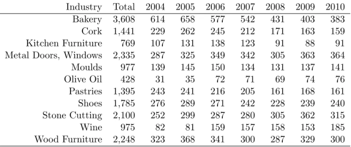
To avoid specifying multiproduct production functions we have selected only

single-product …rms8_{. From these we selected industries that had a su¢ cient}

number of …rms each year to allow estimation and that can also be well de…ned as industries, namely in the consistency of the units of measurement for quantities. Table 1 reports the resulting sample of eleven industries at …ve and seven CAE digits. Further details on data construction are contained in the Data Appendix.

Industry Total 2004 2005 2006 2007 2008 2009 2010 Bakery 3,608 614 658 577 542 431 403 383 Cork 1,441 229 262 245 212 171 163 159 Kitchen Furniture 769 107 131 138 123 91 88 91 Metal Doors, Windows 2,335 287 325 349 342 305 363 364

Moulds 977 139 145 150 134 131 137 141 Olive Oil 428 31 35 72 71 69 74 76 Pastries 1,395 243 241 216 205 161 168 161 Shoes 1,785 276 289 271 242 228 239 240 Stone Cutting 2,100 252 299 287 280 305 362 315 Wine 975 82 81 159 157 158 153 185 Wood Furniture 2,248 323 368 341 300 287 329 300 Table 1: Sample size per industry and year.

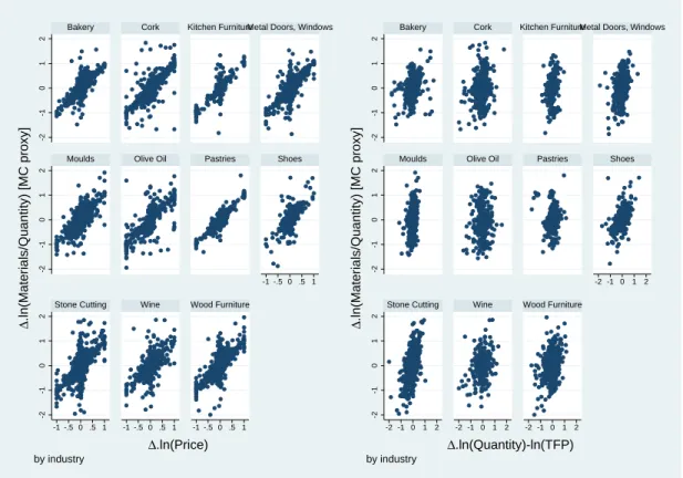
As explained, we use the ratio of input materials to physical output as a …rst proxy for marginal costs. A large ratio means that more inputs are required to produce a given set of units, e.g. if ‡our is used in great amounts to produce x kg of bread, the marginal cost of producing bread is high. Figure 1 reports how

marginal costs vary with output (net of TFP) and prices9. All variables are in

…rst di¤erences so that these are e¤ectively within-…rm (year on year) variations.

8_{Around 25 per cent of the sample are single-product …rms and 45 per cent produce two}

products

First, we can observe that the proxy for marginal costs increases with quanti-ties. Assuming that Portuguese …rms are pro…t-maximizing, we expect marginal costs to increase with production, at least in the short run, as there are …xed inputs (e.g. capital stock). It is thus di¢ cult to increase production in the short run without increasing marginal costs. This in‡exibility will be a fundamental source of the cyclical component.

Second, we can also observe that this proxy for marginal costs increases with prices. This is expected, as …rms increase prices when their marginal costs in-crease. If prices increase more (less) than proportionally, then markups (p=c) will increase (decrease) with prices. The simple framework presented in the previous section, considering both demand and supply shocks, allows us to interpret the basic evidence above through the lens of a structural model. This allows us to disentangle the e¤ect of supply and demand shocks on prices, output and markups. Notice the importance of having detailed micro-level data for single product …rms in dealing with the aggregation problem of average markups. A …rm pro-ducing two products with distinct cyclical behaviors may show at the aggregate level an acyclic average markup due to the changing composition of its revenues as it reallocates inputs from one to the other product. The same occurs at the industry, and the national level.

5

Empirical estimates for TFP and demand

5.1

Production function

We now present the estimation results for Equation [8] using both linear and cubic

-2 -1 0 1 2 -2 -1 0 1 2 -2 -1 0 1 2 -1 -.5 0 .5 1 -1 -.5 0 .5 1 -1 -.5 0 .5 1 -1 -.5 0 .5 1

Bakery Cork Kitchen FurnitureMetal Doors, Windows

Moulds Olive Oil Pastries Shoes

Stone Cutting Wine Wood Furniture

D .ln(Materials/Quantity) [MC proxy] D.ln(Price) by industry -2 -1 0 1 2 -2 -1 0 1 2 -2 -1 0 1 2 -2 -1 0 1 2 -2 -1 0 1 2 -2 -1 0 1 2 -2 -1 0 1 2

Bakery Cork Kitchen FurnitureMetal Doors, Windows

Moulds Olive Oil Pastries Shoes

Stone Cutting Wine Wood Furniture

D

.ln(Materials/Quantity) [MC proxy]

D.ln(Quantity)-ln(TFP) by industry

summary of the results.

Production Function Estimates

Industry RtS Median OID

(H0:RtS=1) Markup p-val

Linear Approximation

Bakery 0.953 0.880*** 0.029 0.044 2.39 0.04 Cork 1.057 0.524*** 0.244*** 0.290*** 0.72 0.65 Kitchen Furnitur 1.001 0.533*** 0.387*** 0.081 0.96 0.77 Metal Doors, Win 0.769*** 0.444*** 0.298*** 0.027 0.77 0.00 Moulds 1.014 0.296*** 0.382*** 0.270** 0.83 0.01 Olive Oil 0.868 0.685*** 0.105 0.078 1.05 0.38 Pastries 1.094* 1.012*** 0.025 0.058 2.37 0.13 Shoes 0.825*** 0.646*** 0.139*** 0.041 1.07 0.00 Stone Cutting 0.806** 0.454*** 0.218*** 0.133* 1.05 0.05 Wine 0.811*** 0.752*** 0.026 0.033* 1.21 0.16 Wood Furniture 0.944 0.669*** 0.107** 0.169*** 1.55 0.00 Cubic approximation Bakery 0.976 0.971*** -0.008 0.013 2.64 0.24 Cork 1.068 0.514*** 0.262*** 0.293*** 0.70 0.68 Kitchen Furnitur 1.058 0.540*** 0.423*** 0.096 0.97 0.80 Metal Doors, Win 0.744*** 0.468*** 0.268*** 0.008 0.81 0.00 Moulds 0.757*** 0.291*** 0.290*** 0.115 0.89 0.34 Olive Oil 0.926 0.819*** 0.086 0.021 1.26 0.53 Pastries 1.086 1.030*** 0.012 0.044 2.42 0.24 Shoes 0.884*** 0.683*** 0.113*** 0.088** 1.13 0.00 Stone Cutting 0.810** 0.463*** 0.212*** 0.134* 1.07 0.03 Wine 0.802*** 0.719*** 0.041 0.042** 1.15 0.15 Wood Furniture 0.950 0.650*** 0.120*** 0.180*** 1.50 0.00 Notes: *** p<0.01, ** p<0.05, * p<0.1

The set of instruments are the logarithms of capital and employment and the lags of the capital stock, output, employment and prices. Instruments include quadratic, cubic terms and interactions. First column reports the test for constant returns to scale.

Table 2: GMM estimates for the production function.

First, the columns presenting the levels of returns to scale (RtS) show us that

most industries are close to constant RtS, i.e. the estimated values for + +

are close to one. Manufacture of metal doors and window frames, shoes, and wine may exhibit slightly decreasing RtS.

Second, we notice that values for are very low, not signi…cantly di¤erent from zero in most cases. Given the short time span of our panel, this is not much of a surprise, as the capital stock does not exhibit enough time variability at the …rm level. We can also observe that values for , the elasticity of materials, are always very high, as expected once we assume that labor, capital, and materials are substitutes.

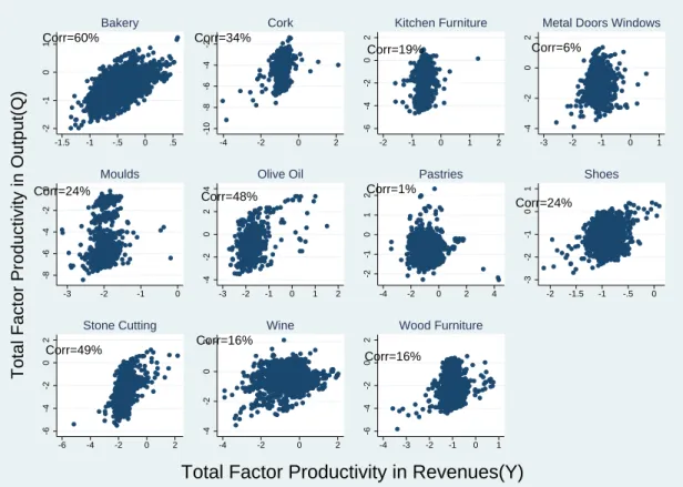
The traditional approach uses revenues as a proxy for output. We compare our estimates to this case. Table B.1 in the Appendix reports the estimated parameters and Figure 2 compares the two TFP estimates. Overall, the two TFP measures exhibit a positive, but low correlation (0.01 to 0.60). The

revenue-based TFP measure (^ay) exhibits much smaller variation when compared to the

quantity-based TFP measure (^aq). This is due to the negative correlation between

e¢ ciency and prices. As such, when companies become more e¢ cient, their ^aq

increases and their prices decrease leading to a smaller reduction in (^ay). This is

in line with the …ndings in Foster et al. [2013].

5.2

Cost function

Table B.2 in the Appendix contains a summary of the results when the cost function is estimated directly. Di¤erences in the estimates for the parameters between the cost- and the production-function approach can be attributed to violations of the duality between production and cost functions. Figure 3 shows how the two TFP estimates compare to each other. Correlations are above 0.90 for all industries, except for metal doors and windows for which the correlation is 0.79.

Corr=60% -2 -1 0 1 -1.5 -1 -.5 0 .5 Bakery Corr=34% -10 -8 -6 -4 -2 -4 -2 0 2 Cork Corr=19% -6 -4 -2 0 2 -2 -1 0 1 2 Kitchen Furniture Corr=6% -4 -2 0 2 -3 -2 -1 0 1

Metal Doors Windows

Corr=24% -8 -6 -4 -2 0 -3 -2 -1 0 Moulds Corr=48% -4 -2 0 2 4 -3 -2 -1 0 1 2 Olive Oil Corr=1% -2 -1 0 1 2 -4 -2 0 2 4 Pastries Corr=24% -3 -2 -1 0 1 -2 -1.5 -1 -.5 0 Shoes Corr=49% -6 -4 -2 0 2 -6 -4 -2 0 2 Stone Cutting Corr=16% -4 -2 0 2 -4 -2 0 2 Wine Corr=16% -6 -4 -2 0 2 -4 -3 -2 -1 0 1 Wood Furniture

Total Factor Productivity in Output(Q)

Total Factor Productivity in Revenues(Y)

Figure 2: Comparison of TFP estimates using the physical output (q) and rev-enuews (y).

Corr=95% -2 -1 0 1 1 2 3 4 5 Bakery Corr=92% -10 -8 -6 -4 -2 -2 0 2 4 6 Cork Corr=98% -6 -4 -2 0 2 -4 -2 0 2 4 Kitchen Furniture Corr=79% -4 -2 0 2 -2 0 2 4

Metal Doors Windows

Corr=98% -8 -6 -4 -2 0 -15 -10 -5 0 Moulds Corr=96% -4 -2 0 2 4 -6 -4 -2 0 2 4 Olive Oil Corr=97% -2 -1 0 1 2 1 2 3 4 5 Pastries Corr=89% -3 -2 -1 0 1 -2 -1 0 1 2 3 Shoes Corr=93% -6 -4 -2 0 2 0 5 10 15 Stone Cutting Corr=91% -4 -2 0 2 0 2 4 6 Wine Corr=97% -6 -4 -2 0 2 -4 -2 0 2 Wood Furniture

Total Factor Productivity via Prod. Func.

Total Factor Productivity via Cost Func.

Figure 3: Comparison of TFP estimates using the cost and the production func-tion.

can observe that the pattern exhibited by the production-function approach is kept here. Footwear and pastries are the only two exceptions.

5.3

The demand function

Figure 4 plots the estimated demand curves for the log-cubic speci…cation in equation [13]. Table B.3 in the Appendix reports the estimated coe¢ cients.

-.5 0 .5 1 1.5 0 1 2 3 4 4 6 8 4 5 6 7 6 8 10 12 -4 -2 0 2 0 1 2 3 2 3 4 5 -3 -2 -1 0 1 -1 0 1 2 3 3 4 5 6 7 -1 -.5 0 .5 -4 -3 -2 -1 0 -26 -24 -22 -20 -21 -20 -19 -18 -17 15 20 25 30 -2 0 2 4 6 -3 -2 -1 0 -15 -14 -13 -12 -11 -2 0 2 4 -4 -2 0 2 -5 -4 -3 -2 -1

Bakery Cork Kitchen Furniture Metal Doors, Windows

Moulds Olive Oil Pastries Shoes

Stone Cutting Wine Wood Furniture

ln(Price)

ln(Quantity)

by industry

Figure 4: Estimated demand functions

Just like TFP, the unobserved demand level has two components due to the Markov speci…cation: inertia (the ‘stock’) and the ‘news’(or ’shock’). Note that we do not impose any type of orthogonality between the unobserved demand and supply components. In fact, the demand level is a stock and it might be positively

correlated with the TFP level (also the stock). That is because more productive companies (stock) also face a larger demand (stock) for their products. This is consistent with the estimated correlations for the productivity and demand components. The correlation between the demand stock ( ) and the TFP stock (a) is 0.44, while the correlation between the demand shock (") and the TFP shock ( ) is 0.01. Demand is positively correlated with TFP while the correlation between the ’news’to demand and the ’news’to TFP is negligible.

6

Markups

6.1

Markups construction

Finally, we report estimates for the markups. Markups, are known directly from the data up to a constant. In the case where labor is also fully ‡exible, the following equality holds

t = F m t + F `t sm t + s`t = F m t sm t = F ` t s` t .

Figure 5 reports the results comparing the markups obtained using the labor share, with those obtained using the intermediate input share. If both inputs

were fully ‡exible, we would expect the markups to be on the 45o line since

F m

sm t =

F `

s`

t (or some other line through the origin when the estimated elasticities

are biased). What we observe is quite the opposite, the relation is negative and not positive. The observed negative correlation between the markup via labor and intermediate input share can be explained by cross-sectional variation in production technologies, i.e., input substitution. In other words, di¤erent …rms

use di¤erent production technologies and the production coe¢ cients ( F ` _and

F m_{) are …rm speci…c. In this case}

F m sm t = F ` i F m i F m F ` F ` s` t = _i F ` s` t

In estimation we assume they are the same across all …rms in the same industry.

A …rm with a labor coe¢ cient above the average ( F `

i > F `) will probably have an

intermediate input below the average ( F m

i < F m) thus generating the observed

negative correlation. To avoid this we net the markup components from the …rm speci…c component. In particular, we regress the markup of …rm i in period t

( it) on a …rm speci…c e¤ect ( i), a time speci…c e¤ect ( t) and we allow for an

idiosyncratic residual (~x it) x it = x i + x t + ~ x it ,

where x = `; m denotes if markups are calculated using the labor or the

interme-diate inputs share ( `

it= F ` t s` t and m it = F m t sm t ).

In Table 3 we report the mean and standard deviation of the two markups ( `

it

and mit) as well as the mean and standard deviation of the two residuals net from

the …rm and time speci…c components (~`it and ~mit). What we observe is that

while `

it and mit have similar variances, which probably denote the variation in

the …xed e¤ect component x

i, the variance of the labor residual, ~

`

itis much larger

than the variance of the intermediate inputs residual ~m_it. This is consistent with

labor being less ‡exible to adjust, as it re‡ects in the fact that the input share does not match the markup, i.e. when output decreases, intermediate inputs adjust, while labor use does not adjust. We will return to a comparison of the two markup

1 2 3 4 0 1 2 3 4 .5 1 1.5 2 2.5 0 1 2 3 4 0 1 2 3 4 1 2 3 4 1 2 3 4 1 2 3 4 0 1 2 3 4 1 2 3 4 1 2 3 4 0 .5 0 1 2 3 4 1 2 3 4 0 1 2 3 4 0 1 2 3 4 0 1 2 3 4 0 .2 .4 .6 0 1 2 3 4 0 1 2 3 4 0 1 2 3 0 1 2 3

Bakery Cork Kitchen Furniture Metal Doors, Windows

Moulds Olive Oil Pastries Shoes

Stone Cutting Wine Wood Furniture

Mark-up via Materials

Mark-up via Labour

by industry

measures below, when we study the cyclical behavior. x it e x it N Mean s.d. Mean s.d. Intermediate inputs 17,815 1.515 0.825 -0.017 0.320 Labor 17,815 0.768 0.817 -0.010 0.800

Table 3: Mark-ups via labor and intermediate input share: levels and net of …rm and time components.

6.2

The cyclical behavior of markups

6.2.1 In-sample dynamics

Markups are considerably persistent, as reported in Figure 6. Such persistence is stronger in some industries like pastries and bakery, and less in other industries like cork and olive oil. This suggests that the degree of persistence varies with industry characteristics. In particular, this is consistent with industries producing more homogenous goods (e.g. cork and olive oil) being more competitive, which may also explain the smaller dispersion in markups for these industries. These more competitive industries (cork, olive oil) exhibit less persistent markups.

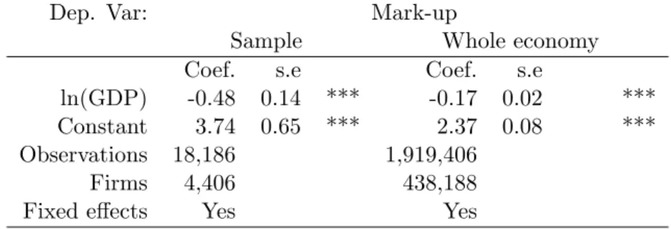
6.2.2 Cyclicality with GDP

As a …rst brief glance at the cyclicality of markups, we project the individual markup on (the log of) real GDP. Table 4 shows a negative correlation of markups with real GDP for the industries analyzed. This is also true when we extend the analysis to all the …rms in IES, using (the change in) the reciprocal of the share of intermediate inputs as a proxy for markups. Thus, this is a preliminary indication that markups tend to be countercyclical with aggregate shocks a¤ecting GDP.

1 2 3 4 0 1 2 3 4 0 2 0 1 2 3 4 0 1 2 3 4 1 2 3 4 1 2 3 4 0 1 2 3 4 0 1 2 3 4 0 1 2 3 4 0 1 2 3 4 1 2 3 4 0 1 2 3 4 0 2 0 1 2 3 4 0 1 2 3 1 2 3 4 1 2 3 4 1 2 3 4 0 1 2 3 4 0 1 2 3 4 0 1 2 3 4

Bakery Cork Kitchen Furniture Metal Doors, Windows

Moulds Olive Oil Pastries Shoes

Stone Cutting Wine Wood Furniture

Mark-up(t)

Mark-up(t-1)

by industry

However, we do not know the source of the aggregate shocks to GDP and how they a¤ect each of the industries. Are ‡uctuations in real GDP demand or supply shocks? To decompose the source of these two e¤ects we need to move to the micro level.

Dep. Var: Mark-up

Sample Whole economy

Coef. s.e Coef. s.e

ln(GDP) -0.48 0.14 *** -0.17 0.02 *** Constant 3.74 0.65 *** 2.37 0.08 *** Observations 18,186 1,919,406

Firms 4,406 438,188

Fixed e¤ects Yes Yes

*** signi…cant at 1%

Notes: The sample results are for the selected industries. In the whole economy the dependent variable is the inverse of the input share for materials and the whole census data is used.

Table 4: Mark-up cyclicality with GPD.

6.2.3 Cyclicality with demand and supply shocks

The previous GDP regression is not the best way of determining the cyclicality of markups. In theory, we can expect di¤erent reactions when …rms face supply and demand shocks. While it is relatively uncontroversial that markups tend to behave procyclically with supply (i.e. TFP) shocks, there is no consensus on the dynamic e¤ect of demand shocks. It is thus important to empirically separate demand and supply shocks. We use the estimated shocks to TFP ( ) and demand (") from the previous section.

Using the estimated demand and TFP shocks, we can now assess how prices, output, and markups respond. Table 5 reports a set of results which are robust across industries. First, prices increase with demand shocks and decrease with

supply shocks. This is what we should expect with standard marginal cost and demand (marginal revenue) slopes, as a demand shock pushes prices up the sup-ply curve, while a supsup-ply shock moves prices down the demand curve. Second, quantities sold (sales) are positively correlated with both supply and demand shocks. Again, this is as expected with standard slopes for the two curves for the same reason. Finally, the markup increases with supply shocks and decreases with demand shocks. An increase in TFP pushes marginal costs down and is translated as a lower price. What the results suggest is that part of the lower marginal cost is absorbed by the company as a larger markup, at least in the short run (consistent with de Loecker et al. [2016]). On the other hand, a shift in demand is associated with an increase in prices and sales. As sales increase, so will marginal costs. These results suggest that the increase in marginal costs is stronger than the increase in prices, following a positive demand shock. We will decompose these e¤ects and analyze them in greater detail in the next section. Our results show that markups are procyclical with TFP shocks and tend to be countercyclical with demand shocks. The exceptions to the latter are olive oil, pastries, and wine, where the results are not statistically di¤erent from zero, i.e. where markups can be classi…ed as acyclical with demand shocks.

Decomposing e¤ects We can decompose the e¤ects of demand and supply

shocks on the markups into its individual e¤ects on prices and quantities using Equations [1] and [2] as follows

Industry Oliv e Oil Bak ery P astries Wine F o ot w ear Cork Stone Metal Do ors Mou lds Kitc hen W o o d Indep. V ar. Cutting Windo ws F urniture F urniture Dep enden t V ariable: .log prices " d 0.289*** -0.026 0.031 0.226*** 0.184* ** 0.307*** 0.221*** 0.317*** 0.313 *** 0.270*** 0.178*** -0.711*** -0.539*** -0.744* ** -0.613*** -0.699*** -0.855*** -0.581*** -0.852*** -0.756*** -0.781*** -0.776*** Dep enden t V ariable: .log quan tit y " d 0.287*** 0.950*** 0.858*** 0.680*** 0.705*** 0.665*** 0.687*** 0.706*** 0.243*** 0.603** * 0.788*** 1.037*** 0.504*** 0.767*** 0.855*** 1.068*** 0.906*** 0.690*** 0.766*** 0.994*** 0.946** * 0.834*** Dep enden t V ariable: .Mark-up " d 0.309** -0.410*** 0.117 -0.147* -0.221*** -0.338*** -1.010*** -0.585*** -0.159** -0.802*** -0.341*** 0.993*** 1.669*** 0.694*** 1.166*** 0.542*** 0.188*** 1.836*** 0.547*** 0.457*** 0.573** * 0.733*** Observ ations 305 2610 1009 703 1361 1044 1504 1638 736 532 1593 Notes: Leas t squares results wi th … rm … xed e¤ ects and time dummies. * p<0.1; ** p<0.05; *** p<0.01 The demand sho cks is calculated as the residual from the demand function and supply sho ck as the residual from the p ro duction function. Mark-ups constructed via pro duction function. Mark-up winsorized at 0.5;10. T a b le 5 : C y cl ic a li ty o f m a rk u p s w it h d em a n d a n d su p p ly sh o ck s (m a rk u p es ti m a te s fr o m p ro d u ct io n fu n ct io n ).

a a

= Pa Cq Qa Ca ₌ Pa _{(1= 1)} Qa _{+ 1= (15)}

In Table 5 we estimated the overall (direct and indirect) e¤ects of demand

shocks on prices ( P _{) and quantities (} Q _{), and the e¤ects of supply shocks on}

prices ( Pa_{) and quantities (} Qa_{). We also estimated the e¤ects on markups of}

demand ( ) and TFP ( aa) shocks. Furthermore, Cq = 1= 1and Ca = 1=

so we can directly use the estimated parameter for from Table 2. Table 6

reports estimates for each of the individual items ( P _; Q _; Pa _and Qa_{) together}

with the cyclicality measures computed from Equations [14] and [15], which can be

compared with the estimated cyclicality measures reported in Table 5, and a.

Overall, the estimated e¤ects of demand and supply shocks on the markup exhibit a remarkable similarity with the estimated e¤ects constructed from Equations [14] and [15]. The results allow us to explain the cyclicality of the markups. Overall, output is sensitive to supply and demand shocks. On the other hand, prices are sensitive to supply shocks but not so much to demand shocks. Together with the increasing marginal cost curves, the results imply that the direct e¢ ciency gains (lower marginal costs) outweight the indirect cost increases and price reductions following an increase to TFP. Markups increase when TFP increases. On the other hand, the cost increase generated by a positive shock to demand is much stronger than the price increases that follow the exact same shock to demand. Markups decrease when demand increases.

Industry Oliv e Oil Ba k ery P astries Wine F o ot w ea r C or k Stone Metal Do ors Moulds Kitc hen W o o d Cutting Windo ws F urniture F urniture 0.309 -0.41 0.117 -0.147 -0.221 -0 .338 -1.01 -0.585 -0.159 -0.802 -0.341 a 0.993 1.669 0.694 1.166 0.542 0.188 1.836 0.5 47 0.457 0.573 0.733 P 0.289 -0.026 0.031 0.226 0.184 0.307 0.221 0.317 0.313 0.27 0.178 Pa -0.711 -0.539 -0.744 -0.613 -0.699 -0.855 -0.581 -0.852 -0.756 -0.781 -0.776 Q 0.287 0.95 0.858 0.68 0.705 0.665 0.68 7 0.706 0.243 0.60 3 0.788 Qa 1.037 0.504 0.767 0.855 1.068 0.90 6 0.69 0.766 0.994 0.946 0.834 0.685 0.88 1.012 0.752 0.646 0.524 0.454 0.444 0.296 0.533 0.669 Computed cyclicalit y measures 0.157 -0.156 0.041 0.002 -0.202 -0.297 -0.605 -0.567 -0.265 -0.258 -0.212 a 0.272 0.529 0.253 0.435 0.264 0.23 0 0.792 0 .4 41 0.258 0.266 0.306 Notes: = ( P (1 = 1) Q ) and a = ( Pa (1 = 1) Qa + 1 = ) T a b le 6 : E ¤ ec t d ec o m p o si ti o n .

6.3

Intermediate inputs

vs. labor

Given the previous results from Figure 5 and Table 3, we would expect that markups obtained using the labor share would behave very di¤erently from the markups obtained from the intermediate input share. This is because as output increases with a given shock, the labor share would decrease as labor does not fully adjust to its optimal level and create a wedge, while the share of intermediate inputs should stay constant at its optimal level. Table 7 shows that the behavior of the markups using the labor share is very di¤erent, even when we use the Nekarda and Ramey [2013] correction to account for the labor wedge of overtime. The correction reduces the cyclicality of the markup but it does not solve the fundamental irresponsive nature. The markups calculated via the labor share are procyclical with the demand shock. This is expected since when faced with an unexpected demand shock, …rms increase output but cannot increase labor by the optimal amount. The labor share goes down and the calculated markup goes up. But to increase the output, …rms have to substitute the increase in labour with an increase in intermediate inputs.

7

Conclusion

We used a rich …rm-level database with a panel of Portuguese industries where information on prices allowed us to separate demand from supply shocks. To do so we developed a new identi…cation mechanism that uses the existence of demand shocks to address the multicollinearity problem that is common in the production function literature. We have then used our estimated shocks to measure their implications for responses on prices, quantities sold, and markups.

Industry Oliv e Oil Bak ery P a str ies Wine F o ot w ea r Cork Stone Metal Do ors Moulds Kitc he n W o o d Indep. V ar. Cutting Windo ws F urniture F urniture Dep enden t V ariable: .Mark-up (via in termediate input sh a re) " d 0.309** -0.410*** 0.117 -0.147* -0.221** * -0.338*** -1.010*** -0.585*** -0.159** -0.802*** -0.341*** 0.993*** 1.669*** 0.694*** 1.166*** 0.542*** 0.188*** 1.836*** 0.547*** 0.457*** 0.573*** 0.733*** Dep enden t V ariable: .Mark-up (via lab or share) " d 0.836*** 0.010*** 0.014*** 0.190*** 0.543*** 1.281*** 0.667*** 1.069*** 0.638*** 1.300*** 0.210*** 0.229** -0.001 -0.001 -0.093 0.307*** 0.074 0.061*** -0.159* ** 0.299*** 0.21 2*** 0.023*** Dep enden t V ariable: .Mark-up (via lab or share, Nek arda and Ramey correction) " d 0.487*** 0.018*** 0.017*** 0.107** 0.385*** 1.019*** 0.464*** 0.750*** 0.509*** 0.940*** 0.133*** 0.128 -0.003** 0.000 -0.101** 0.241*** 0.085 0.043** -0.104*** 0.256*** 0.160*** 0.014** Observ at io n s 305 2610 1009 703 1361 1044 1504 1638 736 532 1593 Notes: Least squares results w ith … rm … xed e¤ ects and time dummies. * p<0.1; ** p<0.05; *** p<0.01 The demand sho cks is calculated as the residual from the demand func tion and supply sh o ck as the residual from the pro duction fu nction. Mark-ups constructed via pro duction function. Mark-up winsorized at 0.5;10. T a b le 7 : C y cl ic a li ty o f m a rk u p s w it h d em a n d a n d su p p ly sh o ck s (m a rk u p s u si n g la b o u r sh a re a n d in te rm ed ia te in p u ts ).

A …rst useful result is that both the production- and the cost-function ap-proaches produce similar results. This is encouraging, as the latter may be ex-tended to multi-product …rms with a less stringent set of assumptions.

A second important result is that markups should be constructed using in-termediate input usage, instead of labor. We o¤er evidence that labor exhibits patterns which are not consistent with fully ‡exible adjustment. Public entities should spend more time reporting intermediate input usage for the economy, as it re‡ects economic activity better than employment statistics, which are likely to react with lag.

Finally, our results contribute to the current macroeconomics discussion on the cyclicality of market power when …rms are hit by both demand and supply shocks. We provide evidence of countercyclical markups with shocks to demand and procyclical with shocks to e¢ ciency.

References

D. Ackerberg, K. Caves, and G. Frazer. Structural identi…cation of production functions. MPRA Papers, 38349, 2006.

A. Afonso and L. Costa. Market power and …scal policy in oecd countries. Applied Economics, 45:4545–4555, 2013.

R. Barro and S. Tenreyro. Closed and open economy models of business cycles with marked up and sticky prices. Economic Journal, 116:434–456, 2006. S. Berry, J. Levinshon, and A. Pakes. Automobile prices in market equilibrium.

F. Bilbiie, F. Ghironi, and M. Melitz. Endogenous entry, product variety, and business cycles. Journal of Political Economy, 120:304–345, 2012.

R. Blundell and J. Powell. Endogeneity in semiparametric binary response models. Review of Economic Studies, 19:321–340, 2004.

S. Bond and M. Soderbom. Adjustment costs and the identi…cation of cobb douglas production functions. IFS Working Papers, WP05/04, 2005.

G. Calvo. Staggered prices in a utility-maximizing framework. Journal of Mone-tary Economics, 12:383–398, 1983.

L. Costa. Endogenous markups and …scal policy. Manchester School, 72 Supple-ment:55–71, 2004.

J. de Loecker. Recovering markups from production data. International Journal of Industrial Organization, 29:350–355, 2011.

J. de Loecker, P. Goldberg, A. Khandelwal, and N. Pavnick. Prices, markups, and trade reform. Econometrica, 84(2):445–510, 2016.

C. Edmond and L. Veldkamp. Income dispersion and counter-cyclical markups. Journal of Monetary Economics, 56:791½U804, 2009.

R. Feenstra. A homothetic utility function for monopolistic competition models, without constant price elasticity. Economics Letters, 78:79–86, 2003.

L. Foster, J. Haltiwanger, and C. Syverson. The slow growth of new plants: Learning about demand? Mimeo, 2013.

J. Galí. Monopolistic competition, business cycles, and the composition of aggre-gate demand. Journal of Economic Theory, 63:73–96, 1994.

A. Gandhi, S. Navarro, and D. Rivers. On the identi…cation of production funtions: How heterogeneous is productivity? Mimeo, 2013.

S. Gilchrist, R. Schoenle, J. Sim, and E. Zakrajsek. In‡ation dynamics during the …nancial crisis. FEDS Discussion Series, 012, 2014.

R. Hall. Market structure and macroeconomic ‡uctuations. Brookings Papers on Economic Activity, 2:285–322, 1986.

R. Hall. By how much does gdp rise if the government buys more output? Brook-ings Papers on Economic Activity, 2:183–231, 2009.

I. Hendel and A. Nevo. Sales and customer inventory. Rand Journal of Economics, 37(3):543–561, 2006.

Y. Hu and M. Shum. Nonparametric identi…cation of dynamic models with un-observed state variables. Journal of Econometrics, 171:32–44, 2012.

N. Jaimovich. Firm dynamics and markup variations: Implications for sunspot equilibria and endogenous economic ‡uctuations. Journal of Economic Theory, 137:300–325, 2007.

F. Juessen and L. Linnemann. Markups and …scal transmission in a panel of oecd countries. Journal of Macroeconomics, 34:674–688, 2012.

T. Klette and Z. Griliches. The inconsistency of common scale estimators when output prices are unobserved and endogenous. Journal of Applied Econometrics,

J. Levinsohn and A. Petrin. Estimating production functions using inputs to control for unobservables. Review of Economic Studies, 70:317–341, 2003. N. Mankiw. Small menu costs and large business cycles: A macroeconomic model

of monopoly. Quarterly Journal of Economics, 100:529–539, 1985.

N. Mankiw and R. Reis. Sticky information versus sticky prices: A proposal to replace the new keynesian phillips curve. Quarterly Journal of Economics, 117: 1295–1328, 2002.

J. Marschak and W. Andrews. Random simultaneous equations and the theory of production. Econometrica, 12:143½U205, 1944.

J. Martins and S. Scarpetta. Estimation of the cyclical behaviour of mark-ups: A technical note. OECD Economic Studies, 34:173–188, 2002.

C. Nekarda and V. Ramey. Industry evidence on the e¤ects of government spend-ing. American Economic Journal: Macroeconomics, 3:36–59, 2011.

C. Nekarda and V. Ramey. The cyclical behavior of the price-cost markup. NBER Working Paper, 19099, 2013.

G. Olley and A. Pakes. The dynamics of productivity in the telecommunications equipment industry. Econometrica, 64:1263½U1297, 1996.

A. Pozzi and F. Schivardi. Demand or productivity: What determines …rm

growth? Rand Journal of Economics, 47(3):608–630, 2016.

M. Ravn, S. Schmitt-Grohé, and M. Uribe. Macroeconomics of subsistence points. Macroeconomic Dynamics, 12:136–147, 2008.

J. Rotemberg. Sticky prices in the united states. Journal of Political Economy, 90:1187–1211, 1982.

J. Rotemberg and M. Woodford. Markups and the business cycle. NBER Macro-economics Annual, 6:63–128, 1991.

J. Rotemberg and M. Woodford. The cyclical behavior of prices and costs. In J. Taylor and M. Woodford, editors, Handbook of Macroeconomics, volume 1B, pages 1051–1135. Elsevier, Amsterdam, 1999.

J. Wooldridge. On estimating …rm-level production functions using proxy variables to control for unobservables. Economics Letters, 104:112–114, 2009.

A

Appendix: Data

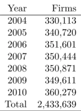
The dataset is obtained using two sources. The …rst source is a census of com-panies (IES) which includes all resident …rms, excluding the …nancial sector and holding companies. The IES covers around 1 million companies per year for the period 2004-2010. Around seven hundred thousand are private individuals which have a simpli…ed reporting and are excluded from the analysis. These are small businesses without obligations of maintaining an organized accounting (only to-tal revenues and number of workers is reported). Some examples are hairdress saloons, restaurants, cafes, carpenters, construction and related services, auto repair, auto sales, wholesale, diverse retail, lawyers, accountants, consultants, ar-chitects, educational services, medical services, etc. We are left with the universe of registered companies in Portugal with organized accounting of over three

hun-Year Firms 2004 330,113 2005 340,720 2006 351,601 2007 350,444 2008 350,871 2009 349,611 2010 360,279 Total 2,433,639

Table A.1: Number of …rms per year for the IES database.

dred thousand per year. The IES contains …nancial information (balance sheet, income statement, investment) and some employment statistics.

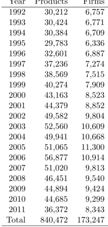
The second source of data is a yearly sample of …rms (IAPI) for the years 1992-2011. The sample contains information on revenues and quantities sold at a very detailed 12 digit product level where each …rm can produce multiple products. This consists of three separate sets of data for products sold, intermediate products consumed, and types of energy used.

A.1

Sample selection

Based on the availability of su¢ cient number of observations per year in the IAPI, the following 5 and 7 digit industries were selected: olive oil processing (5 digits), production of bread/bakery (7 digits), production of fresh pastry and cakes (7 digits), wine (7 digits), leather footwear (7 digits), manufacture of cork (5 digits), cutting, shaping and …nishing of stone (5 digits), manufacture of metal doors and window frames (5 digits), manufacture of industrial moulds (5 digits), manufacture of kitchen furniture (5 digits), and manufacture of wood furniture (5 digits). Kitchen furniture is much di¤erent from general wood furniture as it is typically custom made and involves proximity to the …nal customer.

Year Products Firms 1992 30,212 6,757 1993 30,424 6,771 1994 30,384 6,709 1995 29,783 6,336 1996 32,601 6,887 1997 37,236 7,274 1998 38,569 7,515 1999 40,274 7,909 2000 43,163 8,523 2001 44,379 8,852 2002 49,582 9,804 2003 52,560 10,609 2004 49,941 10,668 2005 51,065 11,300 2006 56,877 10,914 2007 51,020 9,813 2008 46,451 9,540 2009 44,894 9,424 2010 44,685 9,299 2011 36,372 8,343 Total 840,472 173,247

Table A.2: Number of products and …rms per year for the IAPI database.

Number of Products Firms % 1 42,743 25% 2 33,855 20% 3 17,521 10% 4 20,646 12% 5 9,127 5% 6 12,115 7% 7 5,623 3% 8 6,947 4% 9 3,350 2% 10+ 21,320 12%

Industry Total IAPI Merged Usable sample sample sample Bakery 4,436 3,627 3,598

Cork 1,523 1,456 1,388

Kitchen Furniture 836 772 655

Metal Doors, Windows 2,518 2,345 2,309

Moulds 979 978 803 Olive Oil 745 538 267 Pastries 1,596 1,406 1,352 Shoes 1,812 1,794 1,776 Stone Cutting 2,168 2,112 2,053 Wine 1,222 1,170 947 Wood Furniture 2,469 2,270 2,169 Note: The usable sample excludes observations

with missing values for the output or inputs.

Table A.4: Number of …rms per industry (total available from the IAPI database, merged and usable sample).

A.2

Data cleaning

Prices are obtained from IAPI by dividing the product revenues by quantities sold. The obtained series is noisy and subject to outliers. To control for outliers the prices are winsorized at the top and bottom of the price distribution (cross

section). Also, per …rm prices (time series) are winsorized at 170%(log prices at

100%). This treatment removes extreme variations in price levels. Price series are then reconstructed using the winsorized price variations and the base …rm price level.

Physical output is constructed using the reported total revenues (from SCIE) divided by the per …rm price level. Employment is the employment level reported in number of workers. Hours worked is only available for 2004-2009, so that is why we only use it for robustness checks. Intermediate inputs are constructed from reported cost of goods sold. The stock of capital is constructed using the

perpetual inventory formula.

kit= (1 t)ki;t 1+ Iit ,

where tis the year by year rate of depreciation and was obtained from the Bank

of Portugal´s statistics, kit is the capital stock of …rm i in period t and Iit is the

investment of …rm i in period t. All capital series are de‡ated using the capital de‡ator series obtained also from the Bank of Portugal´s statistics. The capital stock for the …rst year the …rm is observed in the data is the total gross amount of …xed assets. Finally, labor costs are constructed from reported total gross wages (including social security contributions).

B

Appendix: Tables

Production Function Estimates with Revenues (Y)

Industry RTS Median OID N

p-val Linear Approximation

Bakery 0.96** 0.86 0.07 0.02 2.34 0.91 0.00 2195

Cork 1.000 0.79 0.15 0.07 1.08 0.72 0.19 904

Kitchen Furnitur 1.030 0.79 0.22 0.02 1.42 0.65 0.46 428 Metal Doors, Win 1.03** 0.75 0.22 0.07 1.30 0.76 0.00 1288

Moulds 0.96* 0.58 0.26 0.13 1.62 0.73 0.01 696 Olive Oil 1.003 0.71 0.07 0.22 1.09 0.64 0.54 216 Pastries 0.43*** 0.21 0.18 0.04 0.49 1.02 0.17 723 Shoes 0.96*** 0.75 0.17 0.04 1.24 0.80 0.00 1325 Stone Cutting 0.979 0.69 0.19 0.11 1.58 0.83 0.00 1213 Wine 0.48*** 0.38 0.07 0.03 0.61 1.00 0.14 609 Wood Furniture 1.007 0.81 0.12 0.08 1.86 0.77 0.00 1406 Notes: The set of instruments are the logarithms of capital and employment and the lags of the capital stock, output, employment and prices. Instruments include quadratic, cubic terms and interactions. First column reports the test for constant returns to scale.