Numerical study of the unsteadiness of a ground vortex

UNIVERSITY OF BEIRA INTERIOR

AEROSPACE SCIENCES DEPARTMENT

NUMERICAL STUDY OF THE

UNSTEADINESS OF A GROUND VORTEX

By

Ricardo Bruno Freitas Nunes

Dissertation submitted to the University of Beira Interior

for the Master Degree in Aeronautical Engineering

Thesis developed under supervision of

Professor Dr. Eng.º Jorge Manuel Martins Barata

NUMERICAL STUDY OF THE

UNSTEADINESS OF A GROUND VORTEX

By

Ricardo Bruno Freitas Nunes

Dedicated to my Parents

and

ABSTRACT

Single impinging jets in a crossflow are typical in impingement cooling applications in industry, as well as of the flow beneath a V/STOL aircraft. In this latter application, a primary design consideration is the flow environment induced by the propulsion system during hover with zero or small forward momentum. Ground effect phenomena may occur and change the lift forces on the aircraft, cause re-ingestion of exhaust gases into the engine intake and raise fuselage skin temperatures. An important source of each is the ground vortex which forms far upstream of the impinging jet when the resulting radial wall jet meets a crossflow. Numerical and experimental studies have also been performed in this area. Some were dedicated to the study of the more fundamental configurations: single or multiple impinging jets through a crossflow.

The present thesis extends the analysis of (Pandya, Murman, & Sankaran, 2003) to a wider range of velocity ratios, VR, from 0.065 to 0.2. The impact zone of a wall jet with a

boundary layer was studied computationally using a Reynolds Averaged Navier-Stokes (RANS) approach with the “k-ε” turbulence model. The computational domain corresponds to complete experimental rig of (Cimbala, Billet, Gaublomme, & Oefelein, 1991) and the measured boundary conditions were used. It was found that the gross features of the flow are well predicted, and the fluctuations of the flowfield around the ground vortex occur in a very small region near the wall where the impact between each flow occurs. The computational results showed a cyclic formation of two small secondary vortexes that appear and disappear cyclically around the separation and maximum penetration points of the ground vortex. This result confirms the observation of (Pandya, Murman, & Sankaran, 2003). The frequency of the “puffing” was found to compare well with the experimental results for VR=0.1, and the structure of the impact zone is similar. First, the wall jet fluid

vortex appears. Then it starts to grow blocking the passage of the clockwise rotating fluid of the wall jet, and a new small vortex appears, but now with clockwise vorticity.

A particular result was obtained for VR=0.175. The flow exhibits a periodic behaviour,

but no secondary vortexes are detected. Nevertheless, in this case the frequency was found to correlate well with the values obtained for VR=0.1, 0.125, and 0.15. For the case of

very low velocity crossflow (small VR) the computations exhibit a stationary solution, which

is in agreement with previous experimental results. For strong crossflows (large VR) the

flow is also stationary, although there is a transition region of some unsteadiness without secondary vortexes present. The present work has shown that for a finite interval of velocity ratios between the impinging jet and the crossflow periodic oscillations of the ground vortex are observed. The results indicate a pattern similar to the “puffing” mechanism described by (Cimbala, Billet, Gaublomme, & Oefelein, 1991).

RESUMO

Um jacto incidente em presença de escoamento cruzado é típico em aplicações industriais de arrefecimento assim como em escoamentos que ocorrem por baixo de uma aeronave V/STOL. Nesta última aplicação um dos principais requisitos do projecto a ser tido em consideração é o sistema propulsivo e a sua influência no escoamento ao redor da aeronave quando esta se encontra perto do solo seja em transição para voo horizontal ou pairando sobre o solo. Perdas nas forças sustentadoras podem ocorrer no momento de aterragem/descolagem perto do solo com re-ingestão de gases quentes na admissão do motor, diminuição de pressão nas superfícies inferiores da asa e da fuselagem, contribuindo com um efeito de sucção na aeronave em direcção ao solo. Os gases quentes também são responsáveis pelo aumento de temperatura nos revestimentos da asa e da fuselagem. Os efeitos acima referidos são em grande parte devido a um escoamento que na literatura inglesa é designado de “ground vortex” e que surge devido à presença de um escoamento cruzado (vento ou o próprio movimento da aeronave). O escoamento cruzado quando interage com o jacto de parede radial, resultante do espraiamento do jacto incidente da aeronave, origina o “ground vortex” a montante do ponto de impacto do jacto incidente. Estudos numéricos e experimentais têm sido realizados nesta área. Alguns estudos foram dedicados a configurações fundamentais com múltiplos ou apenas com um jacto incidente na presença de escoamento cruzado. Estudos publicados sobre este tipo de escoamento são reduzidos e os poucos que existem reportam este tipo de escoamento num contexto secundário, pois grande parte da análise é direccionada para o problema do jacto incidente, que tem sido estudado para diversas configurações e condições de operação.

A presente tese amplia a análise feita por (Pandya, Murman, & Sankaran, 2003) para uma gama de razões de velocidades, de 0.065 a 0.2. A zona de impacto do jacto de parede com a camada limite é estudada computacionalmente utilizando “RANS” e sendo

“k-ε” o modelo de turbulência. O domínio computacional condiz com estudo experimental de (Cimbala, Billet, Gaublomme, & Oefelein, 1991) utilizado as correspondentes condições de fronteira. Verificou-se que as características gerais do escoamento são bem determinadas e que as flutuações do campo de velocidades em torno do “ground vortex” ocorrem numa região muito pequena perto do solo, onde a colisão entre os escoamentos se verifica. Os resultados computacionais mostraram uma formação cíclica de dois pequenos vórtices secundários que aparecem e desaparecem ciclicamente em torno dos pontos de separação e de máxima penetração do “ground vortex”. Observou-se que frequência do “puffing” quando comparada com os resultados experimentais apresentou bom resultados para VR=0.1, com um estrutura semelhante da zona de colisão. Primeiro, o

fluido do jacto de parede começa a penetrar a camada limite até aparecer um vórtice muito pequeno com rotação anti-horária. Então este começa a crescer bloqueando a passagem do fluido do jacto de parede com rotação horária aparecendo um novo vórtice de pequenas dimensões, mas agora com vorticidade horária. Este resultados confirma as observações feitas por (Pandya, Murman, & Sankaran, 2003) quando simulou as medições experimentais com um “smokewire” e verificou a separação de dois vórtices em contra-rotação a partir de um ponto.

Um resultado particular foi obtido para VR=0.175. O escoamento exibe um

comportamento periódico mas não são detectados vórtice secundário. No entanto, observou-se que as frequências correlacionam bem com (Cimbala, Billet, Gaublomme, & Oefelein, 1991) para VR=0.1, 0.124 e 0.15. Para o caso de velocidades muito baixas do

escoamento cruzado (pequeno VR) os resultados computacionais exibem uma solução

estacionária, concordando assim com os resultados experimentais anteriores. Para velocidades do escoamento cruzados mais elevadas (grande VR) este é também

estacionário embora haja uma região de transição com alguma instabilidade mas sem presença dos vórtices secundários. Este trabalho mostra que para um intervalo finito de razões de velocidade entre o jacto incidente e o escoamento cruzado são observadas oscilações periódicas da parte do “ground vortex”. Os resultados indicam um patrão semelhante ao mecanismo de “puffing” descrito por (Cimbala, Billet, Gaublomme, & Oefelein, 1991).

ACKNOWLEDGMENTS

This project would never have been completed without the assistance of many other people. I would like to take this opportunity to express my especial thanks and appreciations to my supervisor, Professor Dr. Jorge M. M. Barata, for his guidance, encouragement.

My most sincere thanks must go to Professor Dr. André R. R. Silva. His friendly advice has always been useful and has contributed significantly to the quality of my work.

Thanks to my colleagues and friends who throughout my studies expressed their friendship and support in important moments. Special thanks for all the support and encouragement of Andreia.

I also wish to express gratitude to my parents who worked a lot to ensure that one day I would have the possibility of having my studies. All their support contributed in large part for this thesis.

Ricardo Nunes Covilhã, 2009

CONTENTS

A

BSTRACT

...

I RESUMO

...

III

A

CKNOWLEDGMENTS

...

V

C

ONTENTS

...

VI

L

IST OF

F

IGURES

...

VIII

L

IST OF

T

ABLES

...

IX NOMENCLATURE

...

X

CHAPTER 1 - INTRODUTION

... 1-1

1.1

F

LOWS

S

TUDIED

... 1-1

1.1.1 Interest ... 1-1 1.1.2 Basic Flowfields ... 1-2

1.2

L

ITERATURE

R

EVIEW

... 1-4

1.2.1 Numerical and Experimental studies ... 1-6

1.3

O

BJECTIVES OF THE THESIS

... 1-13

CHAPTER 2 - MATHEMATICAL MODEL

... 2-1

2.1

I

NTRODUCTION

... 2-1

2.2

G

OVERNING

D

IFFERENTIAL

E

QUATIONS

... 2-1

2.3

T

URBULENCE

M

ODEL

... 2-2

2.4

F

INITE

-D

IFFERENCE

E

QUATIONS

... 2-3

2.5

Q

UICK

S

CHEME

... 2-4

2.6

S

OLUTION

P

ROCEDURE

... 2-6

2.7

B

OUNDARY

C

ONDITIONS

... 2-8

2.7.1 Bottom of the West Boundary (Inlet of the Wall Jet) ... 2-8 2.7.2 East Boundary (Inlet of the Crossflow Velocity or Boundary Layer) ... 2-12 2.7.3 South Boundary (Ground) ... 2-12 2.7.4 North Boundary ... 2-12

2.7.5 Top of the West Boundary ... 2-13

2.8

G

RID

I

NDEPENDENCE

... 2-13

CHAPTER 3 - RESULTS

... 3-1

3.1

I

NTRODUCTION

... 3-1

3.2

S

TUDY OF THE

V

R

=

0.1

(U

R

=0.155)

... 3-3

3.2.1 Vertical Profiles ... 3-3 3.2.2 Horizontal Profiles ... 3-7 3.2.3 Flowfield ... 3-10 3.2.4 Variation of the Vortex Core Positions ... 3-15

3.3

P

ARAMETRIC

S

TUDY OF THE

V

ELOCITY

R

ATIO

... 3-16

3.4

D

ISCUSSION

... 3-17

CHAPTER 4 - CONCLUSION

... 4-1

F

UTURE

D

IRECTIONS

... A

LIST OF FIGURES

FIGURE 1.1-JOIN STRIKE FIGHTER F-35B.V/STOL AIRCRAFT WITH AN ILLUSTRATION OF

THE GROUND VORTEX... 1-2 FIGURE 1.2-FLOWFIELDS IN HOVER (KUHN,MARGASON,&CURTIS,2006) ... 1-3

FIGURE 1.3-TRANSITION IN-GROUND EFFECT (STOL OPERATION),(KUHN,MARGASON,&

CURTIS,2006) ... 1-4

FIGURE 1.4-HOVERING ENVIRONMENT FOR JET-POWERED V/STOL AIRCRAFT,(KUHN,

MARGASON,&CURTIS,2006) ... 1-4 FIGURE 1.5-SCHEMATIC OF A TWIN IMPINGING JET FOUNTAIN FLOW,(SARIPALLI,1987) ... 1-5 FIGURE 1.6-GROUND VORTEX FORMED BY IMPINGING JET IN CROSSFLOW,(KNOWLES &

BRAY,1993) ... 1-6 FIGURE 1.7-VISUALIZATION OF THE SMALL VORTEX AND DRAWING OF POSSIBLE

STREAMLINES,(BARATA J.M.,RIBEIRO,SANTOS,SILVA,&SILVESTRE,2008) .. 1-11 FIGURE 1.8-THE FIGURE IS DIVIDED INTO TWO REGIONS.ONE REGION IS NEAR THE

IMPINGING JET.WHILE THE OTHER REGION IS THE AREA WHERE THE WALL JET COLLIDES WITH THE CROSSFLOW.THE SECOND WILL BE ANALYZED IN THIS

THESIS. ... 1-11

FIGURE 1.9-DIAGRAM OF PRESENT CONFIGURATION:GROUND VORTEX FORMED BY A

WALL JET, FROM A JET IMPINGING NORMAL TO THE GROUND, IN A CROSSFLOW; .. 1-14 FIGURE 2.1-NODAL CONFIGURATION FOR THE WEST FACE OF A CONTROL VOLUME

(BARATA,1989); ... 2-5 FIGURE 2.2-STAGGERED ARRANGEMENTS OF VELOCITY COMPONENTS ON A FINITE

-VOLUME GRID (FULL SYMBOLS DENOTE ELEMENT VERTICES AND OPEN SYMBOLS AT THE CENTER OF THE CONTROL VOLUMES DENOTE COMPUTATIONAL NODES FOR THE STORAGE OF OTHER GOVERNING

VARIABLES); ... 2-7

FIGURE 2.3-CONFIGURATION OF THE DOMAIN ... 2-8 FIGURE 2.4-COMPARISON OF VELOCITY VARIATION FOR SEVERAL VALUES OF

DIMENSIONLESS NOZZLE-TO-PLATE SPACING; THE NOMENCLATURE OF THE FIGURE IS DIFFERENT FROM THE USED IN THIS THESIS:VM=UM;UO,C=VJ; R =X;

AND D=DJ(HRYCAK,LEE,GAUNTNER,&LIVINGOOD,1970) ... 2-10 FIGURE 2.5-VELOCITY PROFILE USED IN THE INLET OF THE WALL JET ... 2-11 FIGURE 2.6-DIMENSIONLESS VERTICAL PROFILE OF THE HORIZONTAL VELOCITY

COMPONENT,U, AT A) X/DJ =4 AND B) X/DJ =14.5 FROM THE IMPINGING

POINT ... 2-13 FIGURE 3.1-SEQUENCE OF THE BEHAVIOR OF THE SMALL SECONDARY VORTEX FOUND BY

(SILVA,DURÃO,BARATA,SANTOS,&RIBEIRO,2008) ... 3-2 FIGURE 3.2-VERTICAL PROFILES OF THE HORIZONTAL VELOCITY COMPONENT,U; ... 3-5 FIGURE 3.3-VERTICAL PROFILES OF THE VERTICAL VELOCITY COMPONENT,V; ... 3-6

FIGURE 3.5-HORIZONTAL PROFILES OF THE VERTICAL VELOCITY COMPONENT,V; ... 3-9

FIGURE 3.6-START OF A CYCLE A) STREAKLINES AND B); STREAKLINES AND VELOCITY VECTORS IN THE FRONTAL ZONE OF THE GROUND VORTEX NEAR THE

SEPARATION AND MAXIMUM PENETRATION POINTS FOR VR=0.1 ... 3-11

FIGURE 3.7-CONTINUATION OF THE CYCLE A) STREAKLINES AND B); STREAKLINES AND VELOCITY VECTORS IN THE FRONTAL ZONE OF THE GROUND VORTEX NEAR THE SEPARATION AND MAXIMUM PENETRATION POINTS FOR VR=0.1 ... 3-11

FIGURE 3.8-CONTINUATION OF THE CYCLE A) STREAKLINES AND B); STREAKLINES AND VELOCITY VECTORS IN THE FRONTAL ZONE OF THE GROUND VORTEX NEAR THE SEPARATION AND MAXIMUM PENETRATION POINTS FOR VR=0.1 ... 3-12

FIGURE 3.9-CONTINUATION OF THE CYCLE A) STREAKLINES AND B); STREAKLINES AND VELOCITY VECTORS IN THE FRONTAL ZONE OF THE GROUND VORTEX NEAR THE SEPARATION AND MAXIMUM PENETRATION POINTS FOR VR=0.1 ... 3-12

FIGURE 3.10-CONTINUATION OF THE CYCLE A) STREAKLINES AND B); STREAKLINES AND VELOCITY VECTORS IN THE FRONTAL ZONE OF THE GROUND VORTEX NEAR THE SEPARATION AND MAXIMUM PENETRATION POINTS FOR VR=0.1 ... 3-13

FIGURE 3.11-CONTINUATION OF THE CYCLE A) STREAKLINES AND B); STREAKLINES AND VELOCITY VECTORS IN THE FRONTAL ZONE OF THE GROUND VORTEX NEAR THE SEPARATION AND MAXIMUM PENETRATION POINTS FOR VR=0.1 ... 3-13

FIGURE 3.12-CONTINUATION OF THE CYCLE A) STREAKLINES AND B); STREAKLINES AND VELOCITY VECTORS IN THE FRONTAL ZONE OF THE GROUND VORTEX NEAR THE SEPARATION AND MAXIMUM PENETRATION POINTS FOR VR=0.1 ... 3-14

FIGURE 3.13-END OF THE CYCLE A) STREAKLINES AND B); STREAKLINES AND VELOCITY VECTORS IN THE FRONTAL ZONE OF THE GROUND VORTEX NEAR THE

SEPARATION AND MAXIMUM PENETRATION POINTS FOR VR=0.1 ... 3-14

FIGURE 3.14-START OF A NEW CYCLE A) STREAKLINES AND B); STREAKLINES AND

VELOCITY VECTORS IN THE FRONTAL ZONE OF THE GROUND VORTEX NEAR THE SEPARATION AND MAXIMUM PENETRATION POINTS FOR VR=0.1 ... 3-15

FIGURE 3.15-LOCATION OF THE CENTRE OF THE VORTEX A) OF ALL THREE VORTEXES; B)

APPROACH TO THE MAIN VORTEX; C) APPROACH TWO SMALLER VORTEXES; ... 3-16 FIGURE 3.16-COMPARISON OF THE NUMERICAL, EXPERIMENTAL AND THEORETICAL

RESULTS: A)VORTEX CENTER HEIGHT AS A FUNCTION O D THE VELOCITY RATIO,VR-1, AT H/DJ=3; B)LOCATION OF THE SEPARATION POINT AS

FUNCTION OF THE VELOCITY RATIO,VR-1; ... 3-17

FIGURE 3.17-UNSTEADINESS FREQUENCY AS A FUNCTION OF THE VELOCITY RATIO A)VR

AND B)VR-1; ... 3-18

LIST OF TABLES

TABLE 2.1-TURBULENCE MODEL CONSTANT ... 2-3

TABLE 3.1-SUMMARY OF CONDITIONS FOR THE CASE VR=0.1 ... 3-3

NOMENCLATURE

Dj m = Nozzle exit diameter

Vj m/s = Velocity of jet at nozzle exit

Uo m/s = Crossflow Velocity

f Hz = Frequency

H m = Distance from nozzle exit to ground plane

hv m = Ground vortex center height (from ground to center of the main

ground vortex)

hv1 m = Ground vortex center height (from ground to center of the

secondary ground vortex)

hv2 m = Ground vortex center height (from ground to center of the third

ground vortex)

x m = Distance along ground plane, in direction upstream of the jet centreline

xwj m = Wall jet profile

xv m = Main ground center point

xv1 m = Secondary ground center point

xv2 m = Third ground center point

xs m = Ground vortex separation point

xp m = Maximum penetration point of ground vortex

y m = Distance normal to the ground plane ywj m = Height of the wall jet at xwj

y1/2 m = Distance normal to the ground plane where

VR - = Reference crossflow-to-jet velocity ratio, Uo/Vj

UR - = Reference crossflow-to-wall jet velocity ratio, Uo/Um

V m/s = Vertical component of velocity U m/s = Horizontal component of velocity

δ m = Wall jet thickness

δBL m = Boundary Layer thickness

b m = Half-width of the jet

Subscripts:

m = Maximum

Chapter 1

INTRODUTION

1.1

Flows Studied

1.1.1

Interest

The flow of one or more jets through a crossflow has great practical interest in several engineering problems such as the emission of pollutants into the atmosphere through chimneys, the injection of secondary air in the dilution of the combustion chamber a gas turbine, the cooling of blades for turbines or the discharge of liquid waste in rivers. However, in this thesis the most important application is the flow produced by the jet of V/STOL1

Over the latter half of the 20th century, many jet and fan-powered V/STOL aircraft concepts have been proposed. These vehicles depend on jet or fan thrust to provide lift for hover and to provide both thrust an lift in very low-speed flight. These thrust forces are produced by both lifting jets and control jets. As the flight speed increases form hover to wing-borne flight (transition flight), the aerodynamic forces and the moments from conventional wing and tail/canard surfaces become the dominant force generators. In the transition speed regime there is a strong interaction between thrust-induced flowfield and aerodynamic-induced flowfield. The resultant combined flowfields are very complex and

aircraft

1

strongly affect the performance of V/STOL aircraft. Traditionally, experimental investigations of either powered models or flights vehicles have been used to understand and quantify these effects. Recently modern computational-fluid-dynamics (CFD) methods have become a useful tool.

Although many aircraft concepts were built, only two jet types, the Russian Yak-38 lift-plus-lift/cruise concepts and the British-developed Harrier deflected thrust concept, have entered service. Currently a third operational aircraft, the Joint Strike Fighter F-35B, lift-fan-plus-lift/cruise concept, is under development to replace the Harrier.

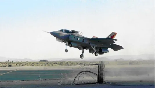
Figure 1.1 – Join strike Fighter F-35B. V/STOL aircraft with an illustration of the ground vortex

1.1.2

Basic Flowfields

An appreciation of the flowfield under and around a jet V/STOL aircraft is necessary to understand the aerodynamic effects of the jet flow as well as the empirical and CFD methods used for estimating them. In transition flight, the freestream deflects the jet flow, and the jet flow alters the freestream flow with profound effects of the lift and moments experienced by the configuration. In hover out-of-ground-effects (figure 1.2) the jet or fan streams entrains air, inducing suction pressures on the lower surface of the aircraft causing a small download or lift loss.

Figure 1.2 - Flowfields in hover (Kuhn, Margason, & Curtis, 2006)

All of the preceding phenomena are present but modified by the proximity of the ground during STOL2

2

Short Take-off and Landing

operation (Figure 1.3). When the jet impinges on the ground, it spreads out in a wall jet flowing radially outward from the impingement point. In addition, the wall jet sheet flowing forward on the ground is opposed by the freestream and rolled up into a ground vortex. This ground vortex induces an additional download, or lift loss, on the configuration, which is at least partially offset by a reduction in the wake vortex system-induced download caused by the truncation of the jet wake by the ground. The positions and strength of the ground vortex are also primary factors in determining the extent of the hot gas, dust and debris, and spray problems that can be generated in STOL operations. These losses may mitigate signicantly the performance of the aircraft in terms of payload and range.

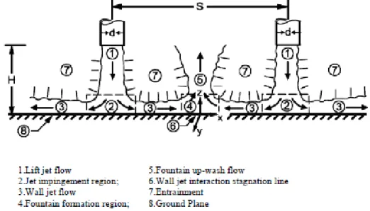
With multiples jets, on the other hand, and upflow or “fountain” is created where the wall jets, flowing outward from the impingement points of adjacent jets, meet. This fountain flow produces a lifting force where it impinges on the lower surface of the aircraft, partially offsetting the download created by the entrainment action of the wall jet flow on the ground. The strength of this lifting force depends on the number and arrangements of the jets. The fountain between a pair of jets is fan shaped, originating from the stagnation line generated where the wall jets, flowing radially outward from the impingement points of the jets, meet.

Figure 1.3 – Transition in-ground effect (STOL operation), (Kuhn, Margason, & Curtis, 2006)

This study seeks to understand the instabilities resulting from a ground vortex, resulting from the collision of a wall jet flow with a crossflow, which has the same velocity profile of a boundary layer flow. As means to try to understand the instability, simulations were performed in CFD for a range of velocities ratio, VR, between the wall jet and the cross flow from 0.065 to 0.2.

From this numerically study were obtain a set of measures of instant velocity led to a general definition of the flowfield, whose detail permitted to evaluate the behaviour of the stagnation zone proving the existence of a small recirculation zone near the stagnation point that may be associated with the appearance of instabilities of the ground vortex.

Figure 1.4 - Hovering environment for jet-powered V/STOL aircraft, (Kuhn, Margason, & Curtis, 2006)

1.2

Literature Review

This section is a literature review of several published investigations until now with focus on the impinging jets in the presence of a cross flow. There are several existing

studies on this matter. The studies can be divided interested in two different areas. The first one distinguishes the studies of one or more impinging jets on flat surfaces involving numerical and experimental studies with or without a crossflow. In the case of multiple jets can be verified the formation of the upwash fountain, illustrated in the following figure:

Figure 1.5 – Schematic of a twin impinging jet fountain flow, (Saripalli, 1987)

The second issue may relate more with the ground vortex although there is a relationship with the first issue, since the ground vortex appears through the impinging jet with the presence of a cross flow, however the main objective is to recognize and describe the whole procedure of the ground vortex. This is the main objective of the thesis that follows. In both issues, it is important to consider the decisive factors in the analysis of flow underneath of an aircraft, these are the velocity ratio, VR and the height of impingement

H/Dj.

This review describes better the contribution of this thesis. Note that only the main researchers working with the application in V/STOL aircraft are cited. Most published studies with importance for problem of V/STOL operations used minimum distances of impingement jet (H/Dj < 8) and low velocity ratio for the crossflow velocity to the wall jet

velocity (VR < 0.1). Some information relevant to the flow formed under a aircraft of V/STOL

operating close to the ground was taken into account in some borderline cases such as H/Dj = 0.4 however without the presence of cross flow (Saripalli, 1983; 1987). Some studies

were conducted to understand the effect of crossflow with the presence of a surface applied at the exit of the nozzle jet. This configuration was used with objective of simulate the lower parts of a V/STOL aircraft, specifically the soffit of the wings and fuselage.

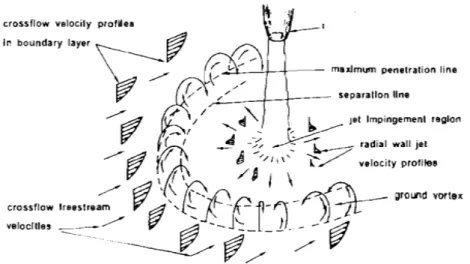
Figure 1.6 – Ground vortex formed by impinging jet in crossflow, (Knowles & Bray, 1993)

Flows that have a curved shape are common in nature. This type of flow can occur for example when a particular flow focuses on a waterproof surface. The surface requires that the flow is deflective in different directions according to the previous figure 1.6.

Other results, corresponding to the existence of a lateral flow, which may cause the deflected of the auxiliary take off jets and the fountain, changing the direction and the application point of the lift force producing moments of "diving" and "rolling" making it difficult the control of the aircraft (Barata, Durão, & McGuirk, 1989).

In the situation where the wall jet flow interact with crossflow exist the formation of a highly curved flow, the ground vortex. The formation of this type of flow takes place upstream of the impinging point of the nozzle and is influenced by several parameters such as the height of impingement, the velocity ratio, whether exist the presence or not of a cross flow, the geometry of the jet nozzle, etc. Measurements of this type of disposal are unusual, or were described only in the context of a secondary flow compared to studies on flow for impinges jets with different configurations of operation without relevance to V/STOL operations.

1.2.1

Numerical and Experimental studies

(Castro & Brasdshaw, 1976) investigated the structure of a turbulent mixing of a highly curved flow. According to what has been said before we can say that the ground vortex flow is considered a highly curved flow. One factor with difficult properties to research, defined by them, is the extra strain ratesand the production of turbulence by the interaction of normal stress with normal deformation. It is also important to note that an

impinging jet on a flat surface is also qualified as a highly curve flow, since the surface requires the radial deflection in different directions. (Rockwell & Naudascher, 1979) reported that the axisymmetrical jets, we can also insert the impinging jet on a flat surface, can cause changes in the structure of the flow. (Saripalli, 1983) conducted experimental studies of observation for impingement with multiple jets and with and without inclination for different heights (H/Dj ≤ 11), however (Saripalli, 1987) presented velocity profiles and

turbulent quantities, obtained by laser anemometer3

One of the critical issues in powered model testing is proper simulation of the ground environment. A moving belt ground board, with an endless belt moving at the same speed as the freestream, was developed to circumvent the problem. With a fixed ground board the forward-flowing wall jet from the impinging jet can progress further forward against the lower energy air in the boundary layer on the ground board than it would against the full velocity of the freestream. The endless belt ground board serves two purposes. First, it eliminates the boundary layer that would exist on a fixed ground board. This is the purpose cited in (Turner, 1967) and all of the early literature. The second, and equally important purpose the belt, is to provide the scrubbing action the ground applied to the wall jet that is moving forward with the aircraft, as it moves over the ground. This scrubbing action reduces the energy in the forward-flowing wall jet. There have been several investigations and summarizations of the position of the ground vortex and the forward penetration of the wall jet (Kuhn, Del Frade, & Eshleman, 1987) (Lawson, Eyles, & Knowles, 2002) (Stewart). The ground vortex is very unsteady but the forward penetration of the zero pressure line for tests over a moving belt ground board is generally only about that over a fixed ground board.

Numerical studies have also been performed in this area. Some were dedicated to the study of the more fundamental configurations: single or multiple impinging jets through a crossflow.

, regarding the disposal of two impinging jets of water on a surface. The results show a linear growth rate of the cross section of the fountain flow that is independent of the height of impingement, H. Although the heights of the jets are within the parameters of interest for V/STOL operations was not taken into account the effect of a crossflow. This in practical situation of a V/STOL operation may be responsible for phenomena as important as the deflection of the impinging jet and the upwash fountain flow or the formation of a recirculation zone upstream from the impinging point, involving the jet with a horseshoe vortex.

(Van Dalsem & Steger, 1987) developed a numerical study for an impinging jet in a presence of a crossflow and predicted the emergence a flow with the form of a horseshoe

3

around the impinging jet, the horseshoe vortex. The study was carried out for different heights (H/Dj = 3,4,6 and 10) and for a velocity ratio (VR = 0.223). This study found a

connection between the oscillation and the ground vortex, but this analysis was very superficial because they had not many experimental data.

Cimbala et al (1988) conducted a study of experimental observation of an impinging jet with a crossflow (formation of the horseshoe vortex), which highlights the instabilities found in the ground vortex, indicating that the instability may be related to the vorticity of the shear layer of the impinging jet. Several velocities ratio were studied including 0.1≤

Uo/Vj ≤ 0.4 for each height H/Dj varying between 1 and 4 and was observed that the ground

vortex was moved downstream causing a decrease in their size as Uo/Vj increased. Found

that by placing a plaque at the same level of the nozzle exit of the impinging jet, the ground vortex was forced to move downstream. At the same time, there was a decrease in the size of the ground vortex.

(Knowles & Bray, 1991; 1993) conducted an experimental study for one and two impinging jet in the presence of a crossflow. In their study varied the parameters that affect the position of the ground vortex for H/Dj ≤ 8. Also performed a numerical study but only for

one impinging jet. The same study show to be valid in accordance with experimental studies, however given the fact that the flowfield show some instability, particularly when there was a fountain formed by two impinging jets.

Cimbala et al (1991) made measurements with hot wire and analyzed the frequency spectrum in the ground vortex, noting there was the existence of a bandwidth with some peaks of frequency, resulting from instability at low frequencies (f = 4Hz for H/Dj = 3 and VR

= 0.1). The instability was explained by a phenomenon of cyclic fluctuations discovered, which is called puffing. This phenomenon was reported with a cyclical behaviour of increase and decrease in size of the ground vortex. In the study was not found any correlation linking the puffing with some oscillations discovered in the flowfield. Most of the low frequency oscillations are attributed to the ground vortex since it increases up to a limit imposed by the flowfield, which feeds the vortex ground by using its ability, until exhaust, to provide energy. When the ground vortex reaches the maximum proportions disappears, however, because of the presence of crossflow form is repeated again and so becoming a cyclical process. The instability of the ground vortex give rise to variations in height, especially for low values of VR, where the vortex just casually reaches a height exceeding

eight diameters of a jet for a VR=0.05. In this situation, there is an inverse of the frequency

variation, which tends linearly to zero when VR decreases.

(Harman, Cimbala, & Billet, 1994)) introduced a technique to reduce the size and the instability that the ground vortex presents. This technique was the use of a grid in the transverse plane on the wall-jet, causing a “fence” in form of a horseshoe around the

impinging jet. The study was carried out for Uo/Vj=0.15 where there were good results,

since the size and instability of the ground vortex decreased by more than 70%.

Barata et al.(1987, 1989, 1991, 1994 and 1996 ) conducted studies for low velocities ratio with a plaque at the nozzle exit of the impinging jet for one, two and three jets. Studies show experimental and numerical results. In the experimental study a LDV was used to carry out measurements of velocities ratio VR=0.014, 0.024 and 0.033 and with the

impinging jet heights of H/Dj=3, 4 and 5, however the measurements were performed in

confined crossflow. The work presents an analysis on the turbulent structure in the impingement areas and curvature of the ground vortex. Although it has been a thorough analysis to regions of flow, the results do not show the presence of any bimodal histogram on measurements made with the LDV for a discrete frequency or multiple jets. Thus, the experimental results cannot prove the existence of instability or discrete oscillation. At first look, the results are surprising, however it appears that the instabilities mentioned in the ground vortex were only listed for different settings such as an impinging jet not confined. An extrapolation of the results described by Cimbala et al (1991), which outlines a comprehensive set of data on fluctuations in the case of a non-confined flow, lead to the presented situation of confined flow by Barata et al (1989) a frequency of puffing of the ground vortex about 0.2 Hz for VR=0.033. However, as mentioned, the samples were taken

always with a minimum of 10 000 measured values in the control volume formed by the laser, with a date rate of 100 Hz, which would be sufficient to detect the frequency of puffing and therefore showing that in these conditions should not exist. Using the same kind of extrapolation of the results of Cimbala et al (1991) to the case of Barata et al (1989) the height of the ground vortex should also be H/Dj=6 (3.5 to 9.5). Which would be

impossible because of the available distance between the upper and lower wall of the channel which was H/Dj=3 to 5.

(Lawson, Eyles, & Knowles, 2002) observed the ground vortex formed by an impinging jet in a compressible flow with a crossflow using a PIV4

4

PIV – Particle Image Velocimetry

that the frequency of oscillation of the position of the ground vortex ranged between 2.5 and 5 Hz. Also viewed through a LDA that velocity fluctuated with frequencies between 1 and 30 Hz. The study was carried out for low velocity ratio (0,026<VR<0,053) with a nozzle pressure ratio, NPR,

ranged from 2.3 to 3.7 and with an impingement height H/Dj between 3 and 10. Through

PIV revealed the presence of small secondary vortex. When the ground vortex increased in size this small secondary vortex appeared but when the ground vortex decreased in size this same small vortex disappeared however they could not recognize clearly its location. They described that this flow was quite unstable, but to a better classification was

necessary a higher frequency for data acquisition in PIV. Presumably, these secondary vortexes may be related to the small area of recirculation.

Pandya et al (2003) conducted a numerical study based on experimental results of Cimbala et al (1991). Was simulated an impinging jet in the presence of a crossflow. The Navier Stokes equations were resolved through an OVERFLOW solver, which enabled the use of large time spacing essential for the detection of small frequency like the puffing of the ground vortex. The instabilities found in the numerical study for the ground vortex showed agreement with the instabilities found in experimental studies.

(Barata & Durão, 2004) investigated the ground vortex resulting from an impinging jet in a confined crossflow, having established that the shape, size and location of the ground vortex are dependent on the ratio between the average velocity of the jet exit and the average velocity of cross flow. It identified the presence of two regimes. One is represented by the interaction between the vortex ground and the impinging jet, while in another regime is the ground vortex is upstream of impingement area, not having contact with the impinging jet. It was also described the acceleration of crossflow on the ground vortex results from the blocking phenomenon produced by the (narrowing of the crossflow area of passage) and because of confinement. It was observed that the acceleration of the flow is directly connected with the nozzle exit velocity of the impinging jet. This result indicated that the influence of the wall jet upstream is not limited to the area of the ground vortex, it diffuses in the upward by a mechanism still poorly reported or known. The quantitative results obtained by LDV and by the visualization have none noticeable oscillation of the ground vortex. It was found that the location and size are solely dependent on the velocity ratio VR and distance of impingement H/Dj for the case of confined crossflow. The results suggest that the fact of there is confinement of the flow may reduce any instability that may exist in the ground vortex as was also reported by Cimbala et al (1988). The fact that the study of Cimbala et al (1991) was not applied to the effect of the velocity jet at the nozzle exit, Vj, may be an indication that the velocity ratio between the impingement jet and

Figure 1.7- Visualization of the small vortex and drawing of possible streamlines, (Barata J. M., Ribeiro, Santos, Silva, & Silvestre, 2008)

(Barata & Durão, 2005) found a small recirculation zone upstream of the stagnation point of the vortex ground (through the interaction of a wall jet with the boundary layer) to a velocity ratio of VR=0.58, issue not reported previously.

(Saddington, Knowles, & Cabrita, 2007) witnessed different frequencies of oscillation for the case of fountain flow resulting from two impinging jets in a compressible regime and without crossflow. The nozzle pressure ratio, ranging from 1.05 to 4, with a height of impingement H/Dj=4. The peaks in power spectral density were found for a frequency of

180Hz, which is very different from the reported to the case of the ground vortex, which only appears when there is a crossflow.

Currently Barata et al (2008) in a more detailed analysis of the ground vortex investigated the presence of small secondary vortex (small area of recirculation) located upstream from the stagnation point resulting from the collision of the wall jet flow with the boundary layer (or crossflow). With the same behaviour of the puffing described by Cimbala et al (1991) with a frequency of 8.33Hz. In the study used a velocities ratio VR=0.58.

Figure 1.8 - The figure is divided into two regions. One region is near the impinging jet. While the other region is the area where the wall jet collides with the crossflow. The second will be analyzed in this thesis.

The most complex numerical study reported so far included all the geometrical and flow details by simulating an entire Harrier aircraft Chanderjian et al (2002) and (Smith, Chawla, & Van Dalsem), but experimental validation of the ground vortex prediction was not possible since there were no available data. Numerical studies of single impinging jet were selected as the basic configuration to study the V/STOL hot gas ingestion phenomena due to the presence of the ground vortex Barata et al (1989), (Jiang & McGuirk, 2000) and Page et al. The majority of those numerical studies use a turbulence model based on the eddy viscosity approach. The mean flow field was predicted quite well except the impinging zone where turbulence production was found to be associated with the normal stresses (Barata, Durão, & McGuirk, 1989) and the pressure term in the momentum equations is dominant Barata et al (1991), (Ince & Leschziner, 1990) studied the influence of turbulence modelling by comparing two Reynolds Stress Model formulations and the “k-ε” eddy viscosity model against the experimental results of (Barata J. M., Durão, Heitor, & McGuirk, 1992) and the results emphasis some merits of a second moment of closure model. Tang et al (2002) reported some simulations with an improved RANS5 “k-ε” model, where an excellent agreement with the shear stresses in the impinging region was obtained. These authors mention that because knowledge of the time-dependent behaviour is essential to a complete understanding of the flow field, even advanced RSM6 models still fail to capture all the details. LES7

Hence, the possibility of using computational techniques for preliminary design work of this type of flows may depend on the increasing computer power and more refined LES simulations were also attempted but as far as the penetration distance is concerned no improvement over the RANS prediction was obtained. Recently, (Worth & Yang, 2006) used also LES and concluded that all the models were still inadequate in providing more than the gross features of the mean flow field, and there is still need for further investigation to predict this flow accurately.

Silva et al (2009) studied the impact zone of a wall jet with a boundary layer. This numerical study was obtained using a Reynolds Averaged Navier-Stokes (RANS) approach with the “k-ε” turbulence model for the experimental conditions of Barata et al (2009). The results emphasis the region near the wall that contains the stagnation and the maximum penetration points where was found to be of most interest to the instabilities mentioned before and a detailed set of measurements are needed to better understand the mechanisms involved.

5 _{Reynolds Averaged Navier-Stokes} 6 _{Reynolds Stress Model}

7

techniques. However, since the impinging zone is the region where most of the numerical model difficulties are concentrated, it should be interesting to evaluate the present computational capabilities to simulate a ground vortex flow separately. It would be even more important to understand the basic flow phenomena that provoke the peculiar and most important characteristics of the ground vortex. Therefore, the present thesis is dedicated to the identification of the parameters and relevant regimes associated with instabilities and other secondary effects of a ground vortex flow.

1.3

Objectives of the thesis

This thesis presents a numerical study of a wall jet flow, resulting from a impinging jet on flat plate, using a crossflow without confinement for a range of velocity ratio, VR-1=Vj/Uo,

from 5 to 15.5 for distances from the nozzle exit to the ground plane of, H/Dj, 3.

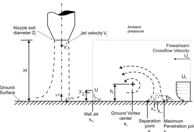
To avoid the influence of the impingement region, done by the impinging jet and according with figure 1.8, the ground vortex is formed by the collision of a wall jet with a boundary layer. The area of greater importance is that which lies further upstream in the vertical plane of symmetry, the transverse component of velocity, w, is zero, so the flow has two-dimensional characteristics. (Gilbert, 1983) used this hypothesis previously in the study of fountain upwash with success. The research presented in this thesis have the general objective to contribute to a better knowledge and understanding of flow characterized by the impingement of jets on plates resulting on a wall jet, in a presence of a crossflow as occurs under a V/STOL jet in terms of landing/takeoff.

The diagram of present configuration is showed in figure 1.9 where the ground vortex is formed by a wall jet, from a jet impinging normal to the ground, in a crossflow.

Following the work done by Cimbala et al (1991) which identified a frequency of the puffing of the ground vortex and Pandya et al (2003) where the work was based on Cimbala et al (1991) confirming the existence of two counter-rotating vortexes separated from the flow passing over the ground vortex.

In the present work analyze of the ground vortex flow is studied using a bi-dimensional configuration for the collision of a wall jet with a boundary layer. The most innovative aspects of this thesis are:

• Establish a relationship between the wall jet velocity and the velocity at the nozzle exit.

• The localization, cycles and the frequency of the ground vortex with a detailed view of what happens near the wall, for a velocity ratio, VR, of 0.1.

• Influence of a very low velocity ratio, VR, ranging from 0.065 to 0.2, on the

flowfield.

• Application of a bi-dimensional numerical method to calculate the collision of the wall jet with the cross flow (boundary layer) with the objective of simplify the calculation and in doing so diminish the calculation time with the same precision of other methods.

• Comparison with experimental Cimbala et al (1991) and numerical Pandya et al (2003) results.

Figure 1.9 - Diagram of present configuration: Ground vortex formed by a wall jet, from a jet impinging normal to the ground, in a crossflow;

Chapter 2

MATHEMATICAL MODEL

2.1

Introduction

This chapter describes a numerical method based on the solution of the conservation laws for mass and momentum, and is a modified version of the method used by (Barata, Durão, & McGuirk, 1989). The method allows good agreement with the measurements of the mean velocity field and the time-averaged governing equations using a standard “k-ε“ turbulence model. In section 2.2 is presented the differential equations to solve together with the equations of the turbulence model, form the system of equations to be solved and in section 2.3 is presented the turbulence model that was used. Then it is describes the obtaining method and the solution of the algebraic equations system discretized which represent the equations of conservation of momentum and the turbulence model equations, including a summary of the numerical scheme and types of boundary conditions applied. In section 2.8 is presented the results of the grid independence.

2.2

Governing Differential Equations

In this section, the basic set of partial equations used is presented. The description of turbulent flow involves the process of obtaining mean quantities applied on the incompressible, isothermal, two-dimensional equations of continuity and the conservative

form of momentum that produces the time-averaged governing equations or more popularly known as the Reynolds Averaged Navier-Stokes, RANS, equations yields.

and the continuity equation as:

Now we have three additional unknowns known as the Reynolds stresses, in the time-averaged momentum equations, which the knowledge is crucial for the calculation of a turbulent flow. It is therefore necessary to introduce a model of turbulence to approximate the Reynolds stresses in terms of quantities of the medium flow, since the deduction of those equations would make appear turbulent correlations of higher order.

2.3

Turbulence Model

This section shows the standard "κ-ε" model (Launder & Spalding, 1974) which was used in this work and summarize some concepts that are associated.

The turbulent diffusion fluxes are approximated with the high number version of the two-equation κ-ε model. It was proposed by Boussinesq (1868) that the Reynolds stresses could be linked to the mean rates of deformation. Can be obtain

The right-hand side is analogous to Newton's law of viscosity, except for the appearance of the turbulent or eddy viscosity μt and turbulent kinetic energy κ. In equation (2.3) the turbulent momentum transport is assumed to be proportional to the mean gradients of velocity.

The turbulent viscosity is not an intrinsic fluid property, but is rather a space and time dependent quantity whose value depends entirely on the local turbulent characteristics of the flow. Based on simple dimensional arguments concerning the relationship between the size and the energetic of individual eddies in fully developed, isotropic turbulence, the model employs the following equation for the turbulence kinematic viscosity:

The values for the turbulent kinetic energy, κ, and the dissipation rate of turbulent energy, ε, are obtained by solving the following transport equations:

The equations contain five adjustable constants Cμ, C1, C2, σκ σε. These constants

have been arrived at by comprehensive data fitting for a wide range of turbulent flows (Launder and Spalding, 1974)

The turbulent model constants expressed in these equations are those, which have provided a good agreement with the experimental results for a wide range of turbulent flow, are:

Cµ C1 C2 σk σε 0.09 1.44 1.92 1.0 1.3 Table 2.1 – Turbulence model constant

The production and dissipation of turbulent kinetic energy are always closely linked in the k-equation (2.5). The dissipation rate ε is large, where the production of κ is large. The model equation (2.5) assumes that the production and dissipation terms are proportional to the production and dissipation terms of the κ-equation. Adoption of such terms ensures that

ε increases rapidly if κ increases rapidly and that decreases sufficiently fast to avoid

nonphysical (negative) values of turbulent kinetic energy if k decreases. The factor ε/κ in the production and dissipation terms makes these terms dimensionally correct in the ε-equation (2.6).

In the present work, this model was used to obtain the numerical results for the flow of the wall jets colliding with the boundary layer.

2.4

Finite-Difference Equations

The solution of the governing equations was obtained using a finite-difference method that used discretized algebraic equations deduced from the exact differential equations that they represent. This discretization involves the integration of the transport equation (2.7)

over an elementary control volume surrounding a central node with a scalar value Φp

(Leonard, Leschziner, & McGuirk, 1978) and as far as the convection term are concerned, it needs the spatial average value of Ф at each cell face.

Where Ф may stand for any velocities, turbulent kinetic energy, or dissipation, and ΓΦ and SΦ take on different values for each particular Ф.

The integrals of volume are converted to integrals of surface for the control volume using Green's theorem; the convection flux for each variable at the cell face must then be estimated based on the value of the variable Φ at the centre of the neighbouring cell.

2.5

Quick Scheme

The representation of values of dependent variables on the faces of the control volume according with the neighbouring values is done with the use of numerical schemes. They are fundamental for the stability and accuracy of the solution, because the use of an infinite number of points that would allow the achievement of exact solution of differential equations of transport is not possible in reality. This way becomes necessary to verify that the equations solutions discretized satisfies some of the proprieties of the exact solution, even for the coarse meshes, presenting a physical realism and a proper overall solution.

The QUICK8

This is achieved by using the quadratic upstream-weighted interpolation to calculate the cell face values for each volume control. (

scheme proposed by Leonard (1979) is free from artificial diffusion and gave the possibility of having coarse meshes with same level of accuracy in the solution than that required for other schemes (e.g. the hybrid scheme).

Figure 2.1) shows the west face of a control volume surrounding a central node with a value ΦP. For this face, using a uniform grid for simplicity, the value of Φ is expressed by

8

P

W

WW

UW

ФP

Ф

ФW

ФWW

if the velocity component Uw is assumed to have the direction shown in Figure 2.1. If Uw were negative ΦWW would be replaced by ΦE in the equation. The first term in equation (2.8) is the central difference formula, and the second is the important stabilizing upstream-weighted normal curvature contribution. Expressing the values of Φ at each cell face with the appropriate interpolation formula and writing gradients also in terms of node values, the finite-difference equation corresponding to equation (2.7) may be written in the general form,

Where

And the summation occurs for the neighbouring points of P.

Figure 2.1 - Nodal configuration for the west face of a control volume (Barata, 1989);

The set of equations for the complete field is solved by this method, the AiΦ coefficients may become negative and stable solutions cannot be obtained. However, the high numerical accuracy of the QUICK scheme and its high sensitivity to the mesh refinement took some authors to search for solutions in the deduction of equations of finite differences, to avoid the instabilities associated with high Peclet numbers (larger than 8/3). (Han, Humphrey, & Launder, 1981) inserted the curvature term (second part of equation 2.8) into the source term and used only the central difference (first part of equation 2.8) contribution to the convective term. This procedure revealed the instabilities of the central differencing schemes, and convergence could only be obtained by using a false transient terms technique, although rather slowly. To avoid the false transient terms and obtains faster convergence, these authors tested different decompositions of quadratic interpolation expressions using part of curvature contribution to evaluate the convective term. These expressions had to be evaluated using the values of Φ calculated at the precious iteration cycle otherwise convergence was very difficult. Moreover, the false transient terms could

not be avoided when calculating turbulent flows and the rate of convergence was deteriorated.

In the present work, diagonal dominance of the coefficient matrix is ensured and enhanced by rearranging the difference equation for the cells where the coefficients AiΦ become negative. This rearrangement consists in subtracting AiΦΦP from both sides of equation (2.9), eliminating the negative contribution of AiΦ and simultaneously enhancing the diagonal dominance of the coefficient matrix (Barata, Durão, & McGuirk, 1989). The source term SUΦ becomes,

where ΦP’ is the latest available value of Φ at node P.

2.6

Solution Procedure

The solution procedure is based on the SIMPLE9

The aim of having a staggered grid arrangement for CFD computations is to evaluate the velocity components at the volume control faces while the rest of the variables governing the flow field, such as the pressure, temperature, and turbulent quantities, are stored at the central node of the control volumes. A typical arrangement is depicted in figure 2.2 on a structured finite-volume grid and it can be demonstrated that the discrete values of the velocity component, u, from the x-momentum equation are evaluated and stored at the east, e, and the west, w, faces of the control volume. By evaluating the other velocity components using the y-momentum and z-momentum equations on the rest of the control volume faces, these velocities allow a straightforward evaluation of the mass fluxes that are used in the pressure correction equation. This arrangement therefore provides a algorithm widely used and reported in the literature (Patankar & Spalding, 1972). In this scheme, a guessed pressure field, p*, is used to solve the momentum equations, which in general does not conform to continuity and it is therefore necessary to solve an equation of Poisson for a variable called the pressure correction. A pressure correction equation, deduced from the continuity equation, is then solved to obtain a pressure correction field, which in turn is used to update the velocity and pressure fields. These guessed fields are progressively improved through the iteration process until convergence is achieved for the velocity and pressure fields.

9

strong coupling between the velocities and pressure, which helps to avoid some types of convergence problems and oscillations in the pressure and velocity fields.

Figure 2.2 - Staggered arrangements of velocity components on a finite-volume grid (full symbols denote element vertices and open symbols at the center of the control volumes denote computational nodes for the

storage of other governing variables);

The system of finite difference equations is solved by applying the algorithm of tridiagonal matrix (Thomas Tridiagonal Matrix Algorithm10

10

The application method was described from the author Barata, 1985

) and the numerical stability and convergence of the solution are improved through the use of relaxation factors, α, so that,

where Φn is the last calculated value of Φ, Φn-1 is the value of the previous iteration and Φ is the value that is used in the following iteration. The values of α were 0.5 for the equations of conservation of momentum and 0.7 for other variables, when the number of points was less than 1000, and 0.3 and 0.5 respectively for more refined meshes.

The accuracy of a numerical solution is determined by the way the partial derivatives in differential equations, are approximate by the algebraic equations discretized, involving an error that can be analyzed based on the Taylor series in development.

2.7

Boundary Conditions

The solution of the equations of conservation of momentum (2.1), equation of continuity (2.2), equation of transport of turbulent kinetic energy (2.5) and the equation of dissipation of turbulent kinetic energy (2.6) in the computational domain considered is essential in a numerical study of a turbulent flow. The elliptical form of the equations considered here requires the prescription of the boundary conditions for all variables at all boundaries of the area. The solution domain, which was used to study the flow of a wall jet colliding with a boundary layer, is shown in figure 2.3 and has five boundaries:

• the inlet of the crossflow (east boundary);

• the inlet of the wall jet (the bottom of the west boundary); • a solid wall (south boundary);

• and two are free boundaries (north boundary and the top of the west boundary).

The location of the border was based on the Cimbala et al (1988 and 1991).

Figure 2.3 – Configuration of the domain

2.7.1

Bottom of the West Boundary (Inlet of the Wall Jet)

At the inflow boundary (the bottom of west boundary), the value of ε was obtained by taking as the characteristic length scale of larger eddies with five percent of the wall jet height at xwj/Dj so the values of the boundary conditions are:

To use the same settings of Cimbala et al (1988 and 1991), there was the need to find a relationship between the velocity at the exit of the nozzle and the resulting velocity after hitting the ground forming the wall jet. The wall jet transition model consist of tree subregions. Where the effect of viscosity is assumed to be negligible except in a region close to the wall and near the edge of the deflected flow is the inviscid deflection region. In the transition region, the effects of viscosity are beginning to dominate and the inner boundary layer and the outer shear flow transitions to a full developed turbulent wall jet. The effects of viscosity of turbulent viscosity dominate and the static pressure through the wall layer is considered ambient or full recovered it is call full developed region. In this region, the nearly similar wall jet develops. The vertical profile of the horizontal velocity component was obtained according to (Hrycak, Lee, Gauntner, & Livingood, 1970) considering the maximum velocity decay along the impingement plate. The maximum velocity Um is the velocity at the boundary between the two flow layers (one where the flow

is influenced by the wall and other where the flow behaves as a free jet).

The analysis follows the method used by (Abramovich, 1963) in his study of the two-dimensional jet. It is based on the assumptions that the flow is incompressible, the ambient is stationary, the flow is in steady state, and the velocity distribution in the turbulent boundary layer is given by the well-known power law,

The value of n adopted was nine due to a favourable gradient of pressure that is associated with the profile.

When the ratio of velocity Um to that the nozzle exit Vj was plotted against a

family of independent of Reynolds number based on nozzle exit velocity was obtained for different values of (see Figure 2.4). The linear portion of the curve represents the maximum velocity decay as,

The length of the deflection region for each value of can be noted at that point where the curves fair into the linear portion.

Figure 2.4 – Comparison of velocity variation for several values of dimensionless nozzle-to-plate spacing; the nomenclature of the figure is different from the used in this thesis: Vm=Um; Uo,c=Vj; r =x; and D=Dj

(Hrycak, Lee, Gauntner, & Livingood, 1970)

Considering that is approximately constant from less or equal to four, this way for it can be used the linear portion of the curve representing the maximum velocity decay showed in equation (2.17). Thus, the west border of the domain is a of the impinging point, where the wall jet is in the fully developed region.

The value of the wall jet thickness δ was then determined as the distance from the wall where . Plots of against could then be made. Such plots of the experimental result are shown in figure 13 of (Hrycak, Lee, Gauntner, & Livingood, 1970) where,

Dimensionless velocity profiles are plotted in figure 16 of (Hrycak, Lee, Gauntner, & Livingood, 1970) against , where y1/2 is the value of y for which

Careful inspection of the experimental data illustrates the validity of the wall jet similarity law. Comparison made between experimental profiles and those of (Glauert, 1956) showed generally good agreement. The data shown in figure 16 of (Hrycak, Lee, Gauntner, & Livingood, 1970) reveal that the experimental profile is lower than Glauert’s in

the outer portion of the jet and is flatter than Glauert’s at the tip, but very similar to (Bakke, 1957) experimental profile. This same figure also showed good agreedement between the data and Abramovich’s relation

for values of ζ/ζ1/2 to about 1.5 and whit b being the width of the jet. Equation (2.20) is

valid only outside the inner turbulent layer. Considering the remaining part of the profile as linear.

Taking into account the equations of this section and the figures that reference was made during the same, the profile used in the inlet of the wall jet (the bottom of west boundary) is

Figure 2.5 – Velocity profile used in the inlet of the wall jet

It was made a comparison with other models for wall-jet profiles (Siclari, Hill, Jenkins, & Migdal, 1980) and (Rajaratnam, 1976) where the results shown that the difference between them does not exceeded 0.5% in relation to the height to the ground

U/U_m y /y1 /2 0 0.2 0.4 0.6 0.8 1 1.2 0 0.2 0.4 0.6 0.8 1 1.2 1.4 1.6 1.8 2 2.2 δ b ζ/ ζ1/2 0 0.25 0.5 0.75 1 1.25 1.5

2.7.2

East Boundary (Inlet of the Crossflow Velocity or Boundary Layer)

At the inflow boundary (east boundary) the value of ε was obtained by taking as the characteristic length scale of larger eddies with five percent of the total height of the domain so the values of the boundary conditions are:

The profile used in the inlet of the crossflow velocity was uniform velocity.

2.7.3

South Boundary (Ground)

Wall boundary (south boundary) conditions were employed for the solid wall bounder of the flow, to represent the ground. In this boundary was used the wall-function method (Launder & Spalding, 1974) at points closer to this, assuming that in the region near the wall, the velocity profile is given by the logarithmic law of the wall and there is local equilibrium between production and dissipation of turbulent kinetic energy. At the same time using the conditions of impermeability of the wall and no-slip, which simply means that the velocities, normal and tangential, are considered to be zero at the solid boundaries.

2.7.4

North Boundary

At the north boundary, the free boundary conditions were employed so the gradients of dependent variables are set to zero

2.7.5

Top of the West Boundary

Similar to the north boundary, at the top of the west boundary, the free boundary conditions were employed so the gradients of dependent variables are set to zero

2.8

Grid Independence

To study the grid independence were simulated four different grids. The first simulation was done for a grid with 29 points in the horizontal and 21 points in the vertical. The following grids were the multiplication of the previous (coarse mesh) grid by the square root of two with a rounded to an integer, which correspond to a reduction in the area of each control volume by half with the increasing of refinement of the mesh. Therefore, was also used the grids 40 x 30, 56 x 42 and another 80 x 60.

Figure 2.6 - Dimensionless vertical profile of the horizontal velocity component, U, at a) x/Dj = 4 and b) x/Dj = 14.5 from the impinging point

The horizontal velocity component, U, was used to test the grid independence. The Figure 2.6 shows the vertical profile of the horizontal velocity component, at x/Dj = 4 and x/Dj = 14.5 from the impinging point with different grids. The diameter of the jet was used to dimensionless the horizontal velocity component. The grid spacing was non-uniform and was used with expansion factors up to 1.2 in both directions, with greater concentration of points near the wall and the entrance of the wall jet. This figures shows the results obtained do not differ significantly from those obtained in the original grid layout can be concluded

U/V_j y /D j -0.1 0 0.1 0.2 0.3 0.4 0.5 0 0.5 1 1.5 2 2.5 3

a)

U/V_j y /D j -0.1 -0.075 -0.05 -0.025 0 0 0.5 1 1.5 2 2.5 3 29 x 21 40 x 30 56 x 42 80 x 60

b)

that the discretization error is at an acceptable level and so the results are independent of numerical influences. Nevertheless, to increase the precision on the evaluation of the wall jet models and to not raise the computational cost performance a finer grid of 56 x 42 was adopted.

Chapter 3

RESULTS

3.1

Introduction

The numerical simulation of wall jet flows, resulting from the impinging jet on a flat plate, through a crossflow is presented in this chapter based on the method described in Chapter 2. The specific aims of the study is to validate numerical solutions of flows typical from V/STOL operations and compared with the experimental and numerical studies reported by Cimbala et al (1988 and 1991) and Pandya et al (2003).

The following section presents the results of the study for the velocity ratio, VR, of 0.1.

One of the most influential parameters in the impinging jets on flat surface is the ratio between the velocity at the nozzle exit and the crossflow, Vj/Uo. In section 3.3, the influence

of these parameters is extends from the analysis of Pandya et al (2003) to a wider range of velocity ratios, VR, from 0.065 to 0.2. In section 3.4 is presented a discussion about the

results presented in the previous sections and with the addition information of the frequencies for the different velocities ratio, VR.

Prior to the detailed measurements experimental visualization studies Silva et al (2008) were performed using a direct digital photography and a smoke generator to produce the tracer particles. Numerical studies was also performed Silva et al (2009). The visualization results of the present complex flow were used to provide a first insight into the nature of the flow and to guide the choice of quantitative measurement locations. The wall jet collides with the boundary layer and is strongly deflected backwards giving rise to an

extremely complex flow, which includes a small secondary vortex flow near the separation point (see figure 3.1), probably due to the roll up of the vorticity of the boundary layer.

Figure 3.1 - Sequence of the behavior of the small secondary vortex found by (Silva, Durão, Barata, Santos, & Ribeiro, 2008)

More detailed visualization (see figure 3.1) studies that confirmed the existence of this second vortex were reported in Silva et al (2008). It was found to be highly unstable with its shape, size, and location varying almost constantly. The behaviour of this small vortex was found to be quite similar to the “puffing” of the ground vortex as reported by Cimbala et al (1991). First the vortex is very small, but growing. The lower part of the boundary layer with counterclockwise vorticity seems to merge into the growing vortex. As the small vortex continues to grow it becomes higher than the boundary layer, and breaks up suddenly while is convected upwards in the direction of the curved flow. Then, a new small vortex appears and starts to grow, and the cyclic process repeats itself. Cimbala et al (1991) attributed the vortex growth to the shear layer vortexes, which convect with the wall jet, and merge into the ground vortex.

Silva et al (2008) found that a different mechanism should be present for the case of higher wall jet-to-boundary layer velocity ratios, because the secondary vortex cannot merge into the deflected flow resulting from the collision of the wall jet with the boundary layer, since the vertical velocity component is always positive above the vortex.

So, probably the unsteadiness reported before is due to an additional (second) small vortex upstream of the ground vortex that due to its extreme small size could not be observed so far, as in the case of high jet-to-crossflow velocity ratios.

The calculations were performed using a time step of 0.04 seconds, firstly over 1,000 seconds (25,000 time steps), to obtain a time averaged solution, and then over 120 seconds (3,000 time steps) to record the continuation or attenuation of the instantaneous perturbations.