Repositório ISCTE-IUL
Deposited in Repositório ISCTE-IUL: 2019-02-28Deposited version: Post-print
Peer-review status of attached file: Peer-reviewed
Citation for published item:
Ruano-Ordás, D., Yevseyeva, I., Basto-Fernandes, V., Méndez, J. R. & Emmerichd, M. T. M. (2019). Improving the drug discovery process by using multiple classifier systems. Expert Systems with Applications. 121, 292-303
Further information on publisher's website: 10.1016/j.eswa.2018.12.032
Publisher's copyright statement:
This is the peer reviewed version of the following article: Ruano-Ordás, D., Yevseyeva, I., Basto-Fernandes, V., Méndez, J. R. & Emmerichd, M. T. M. (2019). Improving the drug discovery process by using multiple classifier systems. Expert Systems with Applications. 121, 292-303, which has been published in final form at https://dx.doi.org/10.1016/j.eswa.2018.12.032. This article may be used for non-commercial purposes in accordance with the Publisher's Terms and Conditions for self-archiving.
Use policy
Creative Commons CC BY 4.0
The full-text may be used and/or reproduced, and given to third parties in any format or medium, without prior permission or charge, for personal research or study, educational, or not-for-profit purposes provided that:
• a full bibliographic reference is made to the original source • a link is made to the metadata record in the Repository • the full-text is not changed in any way
The full-text must not be sold in any format or medium without the formal permission of the copyright holders.
Serviços de Informação e Documentação, Instituto Universitário de Lisboa (ISCTE-IUL) Av. das Forças Armadas, Edifício II, 1649-026 Lisboa Portugal
Phone: +(351) 217 903 024 | e-mail: [email protected] https://repositorio.iscte-iul.pt
1
Improving the drug discovery process by
using multiple classifier systems
David Ruano-Ordása,b,c,d*, Iryna Yevseyevae, Vitor Basto Fernandesf, José R. Méndeza,b,d, Michael T.M. Emmerichc
a Department of Computer Science, University of Vigo, ESEI - Escuela Superior de Ingeniería Informática, Edificio Politécnico, Campus Universitario As Lagoas s/n, 32004 Ourense, Spain
b CINBIO - Biomedical Research Centre, University of Vigo, Campus Universitario Lagoas-Marcosende, 36310 Vigo, Spain
c Multicriteria Optimization, Design, and Analytics Group (MODA), LIACS, Leiden University, Niels Bohrweg 1, 2333-CA Leiden, The Netherlands
d SING Research Group, Galicia Sur Health Research Institute (IIS Galicia Sur). SERGAS-UVIGO
e Cyber Technology Institute, School of Computer Science and Informatics, De Montfort University, Gateway House 5.33, The Gateway, LE1 9BH Leicester, UK
f Instituto Universitário de Lisboa (ISCTE-IUL), University Institute of Lisbon, ISTAR-IUL, Av. das Forças Armadas, 1649-026 Lisboa, Portugal
Email addresses: DRO: [email protected] IY: [email protected] VBF: [email protected] JRM: moncho.mendez.uvigo.es MTME: [email protected] *Corresponding author:
David Ruano-Ordás [Tlf.: +34 988 387015 – Fax: +34 988 387001]
ESEI: Escuela Superior de Ingeniería Informática. Edificio Politécnico. Campus Universitario As Lagoas s/n, 32004 – Ourense – Spain.
3
Abstract
Machine learning methods have become an indispensable tool for utilizing large knowledge and data repositories in science and technology. In the context of the pharmaceutical domain, the amount of acquired knowledge about the design and synthesis of pharmaceutical agents and bioactive molecules (drugs) is enormous. The primary challenge for automatically discovering new drugs from molecular screening information is related to the high dimensionality of datasets, where a wide range of features is included for each candidate drug. Thus, the implementation of improved techniques to ensure an adequate manipulation and interpretation of data becomes mandatory. To mitigate this problem, our tool (called D2-MCS) can split homogeneously the dataset into several groups (the subset of features) and subsequently, determine the most suitable classifier for each group. Finally, the tool allows determining the biological activity of each molecule by a voting scheme. The application of the D2-MCS tool was tested on a standardized, high quality dataset gathered from ChEMBL1 and have shown outperformance of our tool when compare to well-known single classification models.
Keywords
Drug discovery; machine learning algorithms; feature clustering; multiple classifier systems
4
1. Introduction and motivation
Technological advances achieved during recent decades have allowed important findings to be obtained in several highly relevant disciplines such as (i) computer science (Internet (Cohen-Almagor, 2013) and mobile communications (Charlesworth, 2009)), (ii) biology (DNA sequencing (França, Carrilho, & Kist, 2002)), and (iii) biomedicine (such as Face2Gene (Radke, 2017)). More specifically, the high performance achieved by the latest communication and computer systems have turned computer science into one of the most important areas of knowledge due to its wide application in various areas, and in multidisciplinary projects in particular. A clear example of its relevance is reflected in the emergence and development of several interdisciplinary research areas such as bioinformatics (development of new methods and software tools in order to facilitate the interpretation of biological data) or cheminformatics (use of computer and informational techniques to improve the decision making in the area of drug lead identification and optimization).
In fact, the high computational capabilities of computer systems together with the reduced price of storage systems allow achieving advances on processing large amounts of information. In detail, they allow (i) efficiently manipulating huge amounts of information, (ii) applying unused techniques (due to their high computational requirements) and (iii) implementing new exploratory techniques for dealing with large amounts of information (Cao et al., 2018; H. Chen, Engkvist, Wang, Olivecrona, & Blaschke, 2018). Healthcare is one of the most favoured investment and research sectors due to the immense amount of information collected over time (such as diseases, vaccines, drugs or chemical substructures) and its impact on the wellbeing of our society as a whole. The distinct characteristics and structures of information related to the drugs discovery domain (that are completely different from those used in other healthcare areas such as vaccines) together with the immense (and diverse) domain knowledge seriously hamper a straightforward manipulation of the information. This issue forced healthcare companies to intensify efforts and resources in the continuous development and improvement of specific database techniques.
On average, pharmaceutical companies invest approximately 18% (Morgan, Grootendorst, Lexchin, Cunningham, & Greyson, 2011) of their budget into research and development tasks, in order to reduce the time and resources needed to develop new drugs or improve existing ones. In fact, during the period 2015-2017, an average of 38.5 drugs were approved annually, which represents an increase of 47% when compared to the 2008-2013 period (Woodcock, 2017, 2018). Additionally, the market expansion in pharmerging countries and demographic trends in developed countries (with an ageing population) have positioned the pharmaceutical sector at the top of the most profitable industries worldwide. Recent studies (Aitken, 2016; Civaner, 2012) have predicted that the pharmaceutical market will reach nearly USD 1,485 billion by 2021, representing an increase in profits of between 14-17% when compared to revenues achieved during the period 2013-2017.
5
Nevertheless, the complexity and elevated cost of the stages involving the development of the drug and approval process hampers the fast creation of new drugs (Adams & Brantner, 2006). One of the biggest challenges takes place during the first stage (preclinical research), where thousands of compounds are analyzed and combined in order to obtain new potential candidates for development as a medical treatment. Screening methods allow detecting the most promising molecules and reduce efforts wasted for testing futile compounds. As described in (DiMasi, Hansen, & Grabowski, 2003; Hefti, 2008) only 0.1% of the tested compounds achieved promising results according to properties required for a potential candidate to become a drug (i.e., bioactivity, toxicity levels or chemical interactions) and are suitable for further study. Consequently, the knowledge acquired by pharmaceutical laboratories from preclinical research work is highly unbalanced (low number of promising compounds and high number of useless compounds). The particular characteristics of this kind of information (high number of available chemical substructures, their distinct formatting representations and low rate of valid compounds) require the use of customized high-dimensional techniques in order to enhance data interpretation. To alleviate this problem, several researchers (Bajorath, 2002; Lipinski, Lombardo, Dominy, & Feeney, 2001) developed various techniques specially adapted to deal with the specifications of the drugs discovery stages. The other line of research is focused on the development of efficient approaches for selection of most promissing subsets of potential candidates to become a drug based on predicted bioactivity of molecules and their diversity (Yevseyeva et al., 2019). However, after a deep analysis of the state-of-the-art of pharmaceutical domain, we found a lack of high-performance decision-making and prediction techniques suitable for tackling the early pre-clinical stages of the drugs discovery process. The usage of simple Machine Learning (ML) classifiers for screening molecules (represented by the information about their chemical substructures) has been applied with quite good results during the last years. However, we believe that the usage of high-dimensional datasets that often include dependent features has had a significant impact on the performance of classifiers. In fact, the “curse of dimensionality” (Domingos, 2012; Wilcox, 1961; Zhai, Ong, & Tsang, 2014; Zhang, Golbraikh, Oloff, Kohn, & Tropsha, 2006) issue emerged as the complexity of finding linear (and even non-linear) transformations of input variables to assess the target class. Moreover, some classifiers (such as Naïve Bayes) require the independence of input variables. The usage of feature selection schemes could be an adequate form to address this issue. However, the elimination of features could lead to a loss of information. Keeping this in mind, we believe that a Multiple Classifier System (MCS) combining the outputs of several ML classifiers created by using different subsets of features included in the original dataset could improve the screening performance achieved by single classifiers. In this work, we introduce a proposal to create disjoint feature subsets from the original data source (feature-clusters) and maximize the independence of the attributes belonging to each concrete cluster. Hence, classifiers using the MCS would achieve interesting conditions to perform better: (i) lower dimensionality and (ii) independence of input attributes.
Using MCS (Chow, 1965; Woźniak, Graña, & Corchado, 2014) provides adittional advantages. Concretely, they achieve better performance with independence of the amount of available data. Moreover, a combination of classifiers (ensemble of classifiers) trend to outperform the usage of individual classifiers, which entails a better probability of finding an optimal model. Finally, they
6
allow exploiting parallel computing and computer clustering technologies for faster operation while taking advantage of the capabilities/properties provided by each individual classifiers. Despite these interesting features of MCSs, to the best of our knowledge, they have not been applied to automatically select promising chemical substances and improve the drugs discovery process. Keeping this idea in mind and guided by the importance of the preclinical research stage and the lack of techniques to address this problem, we decided to design and develop D2-MCS (Ruano-Ordás, 2018), a novel multiple-classifier system able to automatically determine the biological activity of a specific chemical compound based on its composition (i.e. chemical substructures and physicochemical descriptors). The scientific challenges for the creation of D2-MCS were (i) the choice of an effective but simple method to evaluate the independence of features, (ii) the identification of the number of feature clusters, (iii) training and tuning of classifiers and (iv) the combination of the outputs of classifiers included in the MCS. While this section has presented the motivations of our work, the rest of the paper is structured as follows: Section 2 outlines the most-common ML techniques used for in-silico screening. Section 3 introduces the architectural design of our current biological activity detector software; Section 4 shows the experimental protocol carried out to demonstrate the suitability of our tool. Finally, Section 5 summarizes the main conclusions extracted from this work and outlines future research lines.
2. In-silico screening background
Pre-clinical studies are the first stage of the complex drugs discovery process. The goal of these studies is to identify drug candidates that would be tested in humans (clinical trials) and may become approved drugs. Preclinical studies include a great amount of work and comprise all activities, from the identification of candidate molecules, to the realization of tests of the drug in living cells and animals. Since conventional methods of identifying candidate molecules (screening) are expensive regarding time and cost, it is of key importance to develop high-performance in-silico (computer-based) screening methods. The recent availability of ‘big data’ in cheminformatics makes data-science methods for finding structure-activity relationships (SARs) a highly auspicious direction for in-silico screening of molecular compounds.
In-silico screening (sometimes called virtual screening) has been addressed before with quite good results (Burbidge, Trotter, Buxton, & Holden, 2001; Lavecchia, 2015; Lee, Lee, & Kim, 2017). In (Lavecchia, 2015) a great review of the usage of different ML approaches for ligand-based and structure-ligand-based in-silico screening is introduced. Additionally, these works show the usage of some ML techniques including Support Vector Machines (used in (Burbidge et al., 2001)), decision trees (DT), ensemble methods (such as Adaboost or Random Forests used in (Lee et al., 2017)), Naïve Bayesian based approaches, K-Nearest Neighbor Methods (kNN) and Artificial Neural Networks (ANN, studied in (Burbidge et al., 2001)).
In spite of the great amount of research done in the area of in-silico screening, the opportunity for further development still exists. The performance of classifiers is widely hindered by the unbalanced nature of datasets (which contain only a small amount of active substances), the
7
dimensionality of datasets (more than two thousands of features) and the hidden dependences between the features of the datasets. Moreover, the excellent performance achieved by ensemble methods (especially Random Forests) suggests that using a combination of classifiers has a high potential to improve the achieved results.
Inspired by the above ideas, we designed D2-MCS, a novel screening method able to outperform simple classifiers used in previous works (Burbidge et al., 2001; Lavecchia, 2015; Lee et al., 2017). Next section contains a detailed description of our proposal from the perspectives of software design and method operation.
3. D2-MCS: a novel integrative in-silico model.
In short, the D2-MCS model aims to automatically predict the biological activity of a specific chemical compound through a deep analysis of its chemical substructures. D2-MCS was entirely developed using R programming language since it has become the favorite language for data analysts and scientists all over the world (Gentleman, 1996; Voskoglou, 2017), and was mainly motivated by its: (i) ability to handle complex and large datasets, (ii) capability to easily program and execute complex simulations, and (iii) compatibility with high-performance computer clusters. Additionally, the experimental benchmarking executed in (Fernández-Delgado, Cernadas, Barro, & Amorim, 2014; Statnikov, Wang, & Aliferis, 2008; Tan & Gilbert, 2003) prove the high performance achieved by the classification models provided by the R platform.
Figure 1 shows an illustration of D2-MCS operation, which is divided into three different stages: (i) feature clustering, (ii) model training and hyper-parameter optimization, and (iii) classification results.
8
Figure 1: D2-MCS operation
3.1. Stage 1: Feature clustering
As can be depicted in Figure 1, the first stage incorporates several feature-clustering functions f(x) able to adequately split the dataset attributes (features) into k groups. Motivated by the wide variety of ways of representing and (or) encoding information, the use of customized data-oriented clustering methods is required. To this end, D2-MCS incorporates an interface able to automatically load user-defined feature clustering techniques that can be easily developed using a simple inheritance scheme. By default, D2-MCS provides two simple feature-clustering techniques: (i) BinaryFisherClustering able to deal just with binary features and (ii) MultiTypeFisherClustering capable of managing any type of feature (such as qualitative, discrete and continuous values). To accomplish this task both methods compute the significance value of each binary feature (fb) by using Equation 1.
( ), ( ) 1 . ( . ( , ))
b b b
f binary features s f p value fisher test f class
= −
(1)
where binary(features) stands for the features having binary values and
. ( . ( b, ))
p value fisher test f class computes the significance value of each feature depending on the class through the execution of fisher exact test (Pett, 2015). Since the null hypothesis for fisher.test is the independence of two variables, the 1−p value. could be used as a method to assess the dependence between the fb and the target attribute (class). Then, the ungrouped
features are homogeneously placed in clusters according to the cluster global significance value (designated as
). Equation 2 illustrates how
is calculated for each cluster.9
1, 2,...,
, ( ) b n c b f C C C C C s f =
(2)As can be observed from Equation 2, the global significance of a group C ( c) is computed by adding the partial significance of each feature ( fb) comprising the group
C
. The main goal of the feature clustering stage is to compute a set of clustersG
=
C C
1,
2,...,
C
n
ensuring all clusters (C
i) present a similar global significance (minimize the dispersion of the global significance). The dispersion of the global significance (G) can be assessed by using Equation 3
1 2
,
,
,...,
G
max(
C) min(
C) G
C C
C
n =
−
=
(3)
where max(C)and min(C ) represent the highest and lowest global significance values computed from clusters included in
G
, respectively.To avoid the exploration of all possible distributions of binary features intro clusters, we used a simplified approximation. Hence, the clustering of binary features into a certain number of clusters (nc), require the computation of an ordered feature list using significance function (s f
( )
b ) as sort criterion. Then, the ithelement of a list (i[0,...,#binary(features)−1]) will be placed in the thn cluster (n[0,...,nc−1]) using Equation 4.
(
)
(
%2
)
(
1
)
n= i%nc - i nc
nc
−
(4)where #binary(features) stands for the number of binary features, ÷ stands for the integer division and % stands for the remainder of an integer division.
Finally, the enhanced feature-managing capabilities of the MultiTypeFisherClustering method allows the creation of an additional cluster composed of all the existing non-binary features. Otherwise, the inability of handling these type of features forces BinaryFisherClustering to ignore them and therefore avoid their usage throughout the following stages.
3.2. Stage 2: Train and Tune models
Once the features are successfully grouped into clusters, stage 2 (which involves the training and tuning of models) is automatically executed to determine the best models (and parameters) for each cluster. As can be seen from Figure 1, stage 2 is responsible for building a set of classification models (grouped into 12 different families) over each previously performed feature cluster by using an objective function (called δ) to guide the model parameter-optimization process. This function was created to simplify building of the models according to the classification purpose (such as for minimizing false negative (FN) or false positive (FP) errors). D2-MCS provides possibility of selection one or several objective functions related to different performance metrics well-known in the Machine Learning environment (Coffin & Saltzman, 2000; García, Fernández, Luengo, & Herrera, 2010). Below, Table 1 shows a brief description of the available objective functions together with their associated performance measures.
10
Table 1. Summary of the objective functions provided by D2-MCS tool.
Function
name Measure technique Description
ROC
Receiver Operating Characteristics (Bewick, Cheek, & Ball, 2004; Davis & Goadrich, 2006; Hajian-Tilaki, 2013)
Used to depict the trade-off between the sensitivity and (1-specificity) across a series of cut-off points when the diagnostic test is continuous or on an ordinal scale.
Sensitivity
Sensitivity (Christopher Frey & Patil, 2002; Lalkhen & McCluskey, 2008)
Refers to the ability to correctly identify positive values (e.g. detect patients with a disease).
Specificity Specificity (Lalkhen & McCluskey, 2008)
Computes the ability of the test to correctly identify negative values (e.g. identify patients without a disease).
Kappa Cohen’s Kappa Coefficient (Cohen, 1968; Thompson & Walter, 1988)
Measures inter-rate agreement for qualitative items. It is a more robust measure than a simple percentage agreement calculation, as it takes into account the possibility of the agreement occurring by chance.
Accuracy Accuracy (Makridakis, 1993)
Assess the proportion of true results (both true positives and true negatives) among the total number of cases examined.
MCC
Matthew Correlation Coefficient (Boughorbel, Jarray, & El-Anbari, 2017)
The MCC is, in essence, a correlation coefficient between the observed and predicted binary classifications. Returns a value between −1 and +1. A coefficient of +1 represents a perfect prediction, 0 no better than random prediction and −1 indicates total disagreement between prediction and observation.
PPV Positive Predictive Values (Bewick et al., 2004; Hajian-Tilaki, 2013)
Used to indicate how often a positive test truly represents a true positive.
NPV Negative Predictive Value (Bewick et al., 2004; Hajian-Tilaki, 2013)
Describes the percentage of negative tests being truly negative.
However, the lack of a standardized way of representing the information together with a large number of available performance metrics, require the usage of specific data-oriented methodologies. To mitigate this problem, D2-MCS is equipped with the capability to automatically load new user-defined objective functions in order to build customized data-adapted classification models.
11
After an objective function is selected, stage two automatically executes the classifiers-creation process. To this end, we have user the caret package included in R programing language (Kuhn, 2008). This package internally includes the implementation of different methods of hyper-parameter tuning during the training process. To ensure the convergence of each ML model, the tuning configuration (grid or random search) was selected according to the caret package recommendations. Additionally, during this stage, classifiers are build using a k-fold stratified cross-validation scheme (with k = 10) (Efron & Gong, 1983; Kohavi, 1995) over each previously achieved cluster (C1,C2,...,Cn). D2-MCS provides top 33 most suitable classification models (extracted from caret package) to handle high-dimensional datasets (Fernández-Delgado et al., 2014; Statnikov et al., 2008; Tan & Gilbert, 2003). Table 2 shows a brief description of each classification model together with its corresponding R package and model family.
12
Table 2. Overview of the classification models available in D2-MCS tool.
Model Family Classifier name [R package] R package
Random Forest
Random Forest for High-Dimensional Data
Conditional Inference Random Forest
ranger (Wright & Ziegler, 2017)
party (Hothorn, Hornik, Strobl, & Zeileis, 2018)
Clustering Methods
K-Nearest Neighbors Latent Dirichlet Allocation
caret (Kuhn, 2008)
topicmodels (Grün & Hornik, 2011)
Linear Models
Regularized Generalized Linear Models
Bayesian Generalized Linear Model Penalized Multinomial Regression
glmnet (Friedman, Hastie, & Tibshirani, 2010)
arm (Gelman & Hill, 2006) nnet (Venables & Ripley, 2002)
Support Vector Machines
SVM with Radial Basis Function Kernel SVM with Linear Kernel
SVM with Class Weights SVM with Polynomial Kernel
kernlab
(Karatzoglou, Smola, Hornik, & Zeileis, 2004)
Boosting and Bagging
Adaboost
Boosted Classification Trees Bagged AdaBoost
Bagged CART
Gradient Boosting Machines Extreme Gradient Boosting Gradient Boosting Linear Models
fastAdaboost (Chatterjee, 2016)
ada (Culp, Johnson, & Michailidis, 2006) adabag (Alfaro, Gámez, & García, 2013) caret (Kuhn, 2008)
gbm (Ridgeway, 2004)
xgboost (T. Chen & Guestrin, 2016) mboost (Hothorn et al., 2017)
Tree Models
J48 Trees
CART - R1PARTSE CART - RPART2
RWeka (Hornik et al., 2018)
rpart (Therneau, Atkinson, & Ripley, 2018) rpart (Therneau et al., 2018)
High Dimensional Models
H. Dim. Discriminant Analysis H. Dim. Regularized Discriminant Analysis
Regularized Discriminant Analysis
HDclassif (Berge, Bouveyron, & Girard, 2018)
sparsediscrim (Ramey, 2017) klaR (Friedman, 1989)
Neural Networks
Neural Networks
Neural Networks with Feature Extraction
nnet (Venables & Ripley, 2002)
Probabilistic Models
klaR Naive Bayes Naive Bayes
klaR (Friedman, 1989) naivebayes (Majka, 2018)
Distance Discrimination
Sparse Distance Weighted Discrimination
Linear Distance Weighted Discrimination
sdwd (Wang & Zou, 2018b) kerndwd (Wang & Zou, 2018a)
Rule-Based Models
Random Forest Rule-Based Model Rule-Based Classifier
Conditional Inference Random Forest
randomForest (Breiman, 2001) RWeka (Hornik et al., 2018) RWeka (Hornik et al., 2018)
13
Once the models are fitted with the best-guess hyper-parameters, stage 2 automatically selects the classification model achieving best performance value (according to the objective function). Optionally, to have an overall perspective about the global behavior of all available classifiers, the performance achieved by each model can be plotted graphically.
3.3. Stage 3: Classification
Finally, in stage three previously selected classifiers (best of each cluster) are used to perform the classification task. To this end, the individual results of each classification model are combined in a unique result by applying a specific voting system. Our tool applies the majority voting system due to its adequate balance between performance, resource consumption, and computational speed (Dietterich, 2000; Ruta & Gabrys, 2005; van Erp, Vuurpijl, & Schomaker, 2002). In order to increase the flexibility of the application, the voting system is implemented as a callback function. This scheme allows users to easily test and execute their customized voting strategies.
4. Model evaluation
In order to assess the effectiveness of the proposed model for determining the biological activity of the molecules, we designed and executed a set of experiments involving a set comprising 3925 chemical compounds represented by 2132 descriptors. In order to reduce the elevated cost related to the drugs discovery process, it is important to minimize the number of tests of invalid compounds (biologically inactive compounds). With the aim of minimizing this problem (reducing the number of FN errors), we performed the experimental protocol using MCC and PPV as objective functions. Finally, we implemented a benchmarking comparison of D2-MCS against the model achieving best performance values among those included in Table 2. Our experimental setup together with the selected dataset is introduced in Section 4.1, while Section 4.2 presents and discusses the achieved results.
4.1. Experimental setup
To perform a straightforward and reproducible protocol, we used a standardized, high-quality dataset gathered from ChEMBL2 version 22 based on UniProt accession P34972 (Gaulton et al., 2012). Regarding to activity data potential, duplicates were ignored, no activity or data validity comments were allowed, only data from binding assays and with a pCheMBL value were kept. This led to a dataset composed of 3925 chemical compounds (instances) represented using 2132 features. The first 2048 features epitomize different chemical structures fingerprints (represented using FCFP_6 notation (O’Boyle & Sayle, 2016; Rogers & Hahn, 2010)), while the remaining 84 are associated with several physicochemical descriptors (such as Fractional Polar Surface Area (Ertl, Rohde, & Selzer, 2000; Shrake & Rupley, 1973), Rotatable Bonds (Veber et al., 2002) or Molecular Weight (Tresadern et al., 2017)). Additionally, the set was transformed
14
into a binary classification set where the activity cut-off was defined at a pChEMBL value > 7 (Lenselink et al., 2016) to ensure highly active compounds. Finally, each compound was written into a tab-delimited text file. The final set contained 1977 active compounds and 1948 inactive compounds. Table 3 shows the codification of each feature grouped by type.
Table 3. Feature characteristics and distribution.
Feature type Feature values Nº of features
Chemical substructure fingerprints binary 2048
Physicochemical descriptors
discrete values 50
continuous values 34
Total: 2132
As can be seen from Table 3, each chemical substructure fingerprint is codified using binary notation to indicate its presence (1) or absence (0) for each specific chemical compound. Moreover, the physicochemical descriptors are represented with discrete or continuous values according to the descriptor type and metric representation.
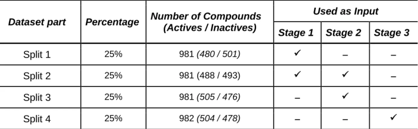
To perform the experimental setup the dataset was randomly divided into four equally distributed splits. Each split comprises 25% of the whole dataset with the same amount of Active and Inactive compounds. Moreover, to avoid model overfitting and therefore ensure realistic classification results, each split is assigned to a specific stage of the D2-MCS process. Table 4 shows a brief description concerning the main characteristics of each split (such as number of compounds or class ratio) together with the relationship among each stage.
Table 4. Dataset division and distribution
Dataset part Percentage Number of Compounds (Actives / Inactives)
Used as Input
Stage 1 Stage 2 Stage 3
Split 1 25% 981 (480 / 501) ✓ ̶ ̶
Split 2 25% 981 (488 / 493) ✓ ✓ ̶
Split 3 25% 981 (505 / 476) ̶ ✓ ̶
Split 4 25% 982 (504 / 478) ̶ ̶ ✓
As can be seen from Table 4, the union of the first two splits are used to accomplish stage one (perform the clustering of features). During this stage, the specific-data-oriented MultiTypeFisherClustering is applied as feature clustering method due to its ability to handle features having different codifications (binary, continuous and discrete). Then, second and third splits are utilized as input for both, performing the model-building and
hyper-parameter-15
optimization processes (stage two). The partial overlapping of data used for the first two stages has been designed to reduce potential coupling troubles while maximizing information available to execute both stages. Finally, the last split is used as a test set to evaluate the performance of our proposal (and is not used for any other purpose to ensure the significance of the results). For comparison purposes, our proposal has been benchmarked against the utilization of simple and ensemble classifiers. The same dataset organization has been used for this purpose. However, in this case, splits 1, 2 and 3 has been applied for training and optimizing purposes while split 4 is utilized for model evaluation purposes.
From a general perspective and given the similarity of the drugs discovery domain with a binary classification problem (i.e., determining the absence/presence of biological activity), there is a wide range of statistical methods available to assess the performance of the classification models (Kosinski, 2013). However, as mentioned in (Baldi, Brunak, Chauvin, Andersen, & Nielsen, 2000), the particular characteristics of this domain requires the usage of adequate problem-oriented statistical methods, in order to ensure a successful and realistic assessment of the achieved results. Following medicinal chemistry experts and authors suggestions (Boughorbel et al., 2017; Powers, 2011), we considered that the most adequate measures to evaluate the final performance of the previously constructed models are PPV and MCC, due to their usage as objective functions during the second stage.
4.2. Results and discussion
To validate and test the performance of our D2-MCS tool correctly, we consider two different scenarios: (i) MCC scenario, where MCC coefficient is used as an objective-function for building the classification model and, (ii) PPV scenario, where PPV measure is considered for the optimization of classifiers. Additionally, in order to demonstrate the suitability of D2-MCS, we also execute a performance benchmarking comparison of our proposal and the simple ML algorithm achieving best performance.
As previously stated, the first stage of the D2-MCS operation uses MultiTypeFisherClustering strategy due to its ability to handle multi-type features. It is important to highlight that obtaining an adequate clustering homogeneity is mandatory to guarantee a good classification performance. To this end, we executed MultiTypeFisherClustering to find a set of feature clusters (
G
) that ensures the minimization of the dispersion of the global significance (
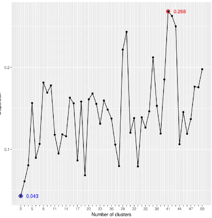
G). For reducing computational requirements we limit the maximum number of clusters included in G to 50 and plotted the best
G achieved with regard of the number of clusters included in G (Figure 2). As can be seen from Figure 2, when grouping the binary features into two clusters, the lowest dispersion is achieved. However, the usage of 41 clusters provided the worst dispersion results. Moreover, a deep analysis of the results depicted in Figure 2 shows two particular aspects: (i) the high dependence between the dispersion and number of cluster divisions, (ii) abrupt changes in the dispersion values for contiguous clustering configurations and (iii) the dispersion is worsened with the increment of the number of clusters (and therefore the limitation of 50 clusters for the configuration seems adequate).16
Figure 2. Dispersion plot for first 50 feature clustering divisions.
In view of the achieved results, the usage of two clusters is the best configuration to minimize the dispersion of the global significance between feature clusters. Following our method, an additional cluster is created to allocate the remaining features (continuous and discrete ones). Finally, non-binary features having constant values were ignored in the classification process, because they are useless.
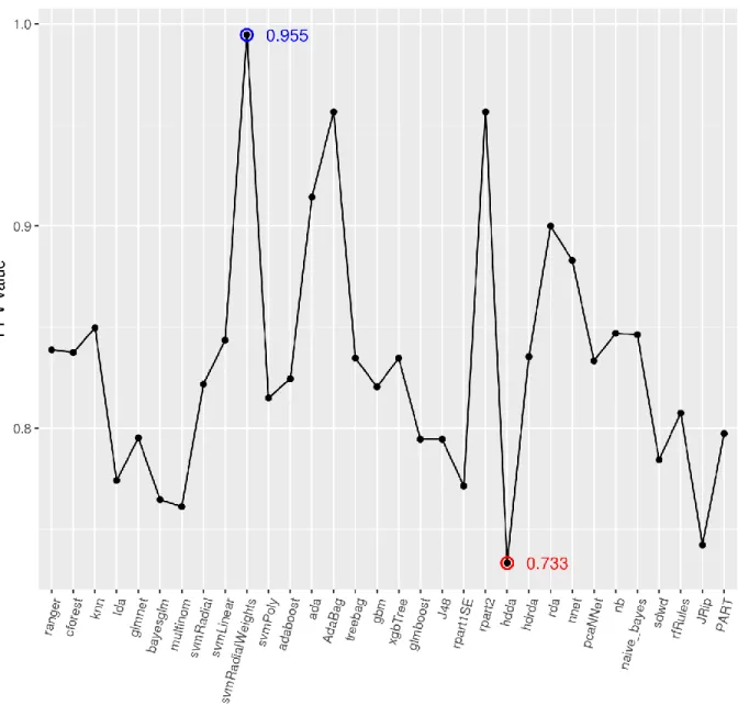
The second step (model building and hyper-parameter optimization) is executed for each of the three previously obtained clusters. Figures 3 and 4 show the performance results achieved for each optimized ML model using PPV and MCC measures as objective functions, respectively.
17
18
19
c) Performance achieved for cluster 3 of 3 (non-binary features).
Figure 3. Performance plot of each ML model for PPV scenario.
As can be noted from results plotted in Figure 3, the performance of each ML model is closely related to the features included in each cluster. Figure 3a svmRadialWeights reveals the great classification performance achieved by svmRadialWeigths classifier (0.975) while AdaBag obtains the worst performance evaluation (0.634). With regard to second feature cluster (see Figure 3b), the best-analyzed model is Adabag (0.978) whilst rpart1SE achieves the poorest evaluation (0.720). Finally, as shown in Figure 3c (third cluster) svmRadialWeights and hdda models achieved the best (0.996) and worst (0.730) performance values, respectively.
Table 5 summarizes the best ML models and hyper-parameter values for each feature cluster. Although svmRadialWeights achieves the highest performance results in two feature clusters,
20
the optimized configurations computed for each of them are significantly different due to their intrinsic characteristics.
Table 5. Hyper-parameter configuration for best ML models using PPV measure.
Cluster number M.L. model Model hyper-parameter values
Cluster 1 svmRadialWeights sigma 0.005277482 C 1.780091 weights 13.66537 Cluster 2 AdaBag maxdepth 1 mfinal 50 Cluster 3 svmRadialWeights sigma 0.02495968 C 0.3483489 weights 13.47197
Figure 4 shows the best performance achieved by ML models using MCC measure to optimize classifier parameters.
21
22
23
c) Performance achieved for cluster 3 of 3 (binary features).
Figure 4. Performance plot of each ML model for MCC scenario.
A brief glance at results included in Figure 4 reveals ranger as the model with the best performance for all clusters. Among the other models, naive_bayes (clusters one and two) and hdda (in cluster three) achieved the worst evaluation results. Table 6 shows a brief summary of the best configuration obtained for ranger for each cluster.
24
Table 6. Hyper-parameter configuration for best ML models using MCC measure.
Cluster number ML model Model hyper-parameter values
Cluster 1 ranger mtry 1026 splitrule extratrees min.node.size 1 Cluster 2 ranger mtry 45 splitrule extratrees min.node.size 1 Cluster 3 ranger mtry 2 splitrule extratrees min.node.size 1
As in the previous scenario (PPV), although ranger model achieves the best performance, the specific configuration details to achieve the best performance for each feature cluster are quite different.
During the third stage, configurations achieved in previous stages are benchmarked against simple and ensemble ML classifiers. As stated before, there are three different classifiers (with their particular outputs) for each scenario (PPV and MCC) and therefore, the final simple classification result for each instance is computed by executing a majority-voting system over the results achieved by each classification model. The primary outcome of the third stage of each scenario comprises the set of confusion matrices achieved that are included in Table 7. The confusion matrix brings together the number of different types of errors and hits including: (i) false positive errors (FP, inactive compounds classified as active); (ii) false negative errors (FN, undetected active compounds); (iii) true positive hits (TP, number of active compounds detected); and (iv) true negative hits (TN, number of inactive compounds correctly classified). Table 7. Confusion matrix for PPV and MCC measures
Reference
Prediction
PPV MCC
Active Inactive Active Inactive
Active 477 382 470 51
25
As reflected from analysis of Table 7, the usage of PPV measure as objective function allows minimizing FP errors at expenses of penalizing the FN ones. The difficulty of finding active compounds in the drugs discovery domain forces the need of minimizing misclassification of potential drug candidates as inactive compounds (FP errors). On the other hand, the usage of MCC allows achieving a balanced value between FP and FN errors. In fact, MCC reduces the number of FN errors up to 3.5 times but increases the FP errors up to 18 times when compared to PPV measure. Taking this fact into account, this measure is suitable for usage in environments where available resources are limited (mainly personal and monetary) and the emergence of FP errors does not cause major problems.
To facilitate the understanding of results included in Table 7, Figure 5 presents a plot including the Accuracy, MCC and PPV measures obtained for each objective function, MCC and PPV, respectively.
Figure 5. Performance comparison plot for both analyzed objective functions.
As can be observed from Figure 5, using MCC as objective function allows to achieve the best Accuracy evaluations due to its good performance when classifying inactive compounds and a good MCC assessment (0.8271 indicates a very strong positive relationship). Otherwise, using PPV as objective function enables achieving the highest PPV results (0.9937) and a quite good MCC evaluation (0.9327). In view of the obtained results, it is easy to highlight the importance of choosing a problem-oriented objective function to achieve the most suitable results.
With the aim of showing the performance gained during the classification stage, we included in Figure 6 a graphical plot highlighting the classification performance achieved for each objective function during both training and testing stages.
26 a) PPV evaluation achieved in stages 2 and 3
(PPV scenario)
b) MCC evaluation achieved in stages 2 and 3 (MCC scenario)
Figure 6. Performance comparison for PPV and MCC scenario.
As can be seen from Figure 6, the classification performance achieved after applying the majority-voting system (indicated as stripped lines) outperforms the results achieved during the training stage. In fact, despite using for testing purposes a dataset never used during previous stages, for MCC (see Figure 6a) classification performance was able to significantly improve best training result (achieved by cluster 2) up to 0.176, while classification performance achieved by PPV improved up to 0.016 the result obtained by cluster 2 (see Figure 6b).
Finally, we performed an experimental benchmarking to assess the suitability of our model against a single best performing ML classification model. In order to simulate the same conditions as used when executing the D2-MCS experimental protocol, classification models described in Table 2 were optimized (with hyper-parameter configuration) using a straightforward 10-fold cross-validation strategy applied over the whole features set composed of the first three dataset parts (splits 1, 2 and 3). Then, using the optimized configuration, models were trained using all instances included in the same splits. From all models in each scenario, we selected the one achieving the best classification performance over the remaining dataset instances (split 4) and compared it with D2-MCS. Below, Table 8 shows the performance results achieved for the best single classifier and D2-MCS. In order to enhance the comparison between models, Table 8 includes the performance result achieved for both models during the optimization/training and testing stages (for MCC and PPV scenario).
Table 8. Performance comparison between D2-MCS and the best single classifiers.
Objective function Model Cluster number Performance measures MCC PPV Optim. and Train Test Optim. and Train Test MCC D2-MCS ranger 1 0.6460 0.8271 ̶ ̶
27 ranger 2 0.6510 (+0.176) ̶ ranger 3 0.6299 ̶ Single classifier ranger ̶ 0.6644 0.6609 (-0.0035) ̶ ̶ PPV D2-MCS svmRadialWeights 1 ̶ ̶ 0.9743 0.9937 (+0.016) AdaBag 2 ̶ 0.9777 svmRadialWeights 3 ̶ 0.9555 Single classifier svmRadialWeights ̶ ̶ ̶ 0.9989 0.9580 (-0.0409)
As can be seen from Table 8, D2-MCS outperforms the best classification model in each cluster. As the execution of training/optimization stage in D2-MCS provides three different performance values (one for each classifier), we computed the performance differential value (included in brackets) as the difference between the result achieved in the testing stage and the maximum value reached during the training/optimization stage. The positive performance difference value achieved by D2-MCS (highlighted in green) indicates the ability to build a suitable knowledge-generalization model. Conversely, although the usage of a single classification model achieves adequate performance results during the training/optimization stage, the negative value of the performance difference (highlighted in red) for both scenarios (using PPV and MCC as objective functions) shows a clear overfitting trend.
5. Conclusions and future work
This work presents D2-MCS, an MCS tool designed to automatically determine the biological activity of molecules based on 2048 chemical substructures (codified using binary values) and 84 physicochemical properties (codified using discrete and continuous values). To successfully address the manipulation of this high-dimensional dataset, D2-MCS performs a 3-stage classification process comprised by: (i) feature clustering, (ii) building and optimizing hyper-parameters of a classification model and (iii) molecule classification. Additionally, we performed an experimental benchmarking comprising two scenarios (using PPV and MCC measures as objective functions) in order to measure the suitability of our D2-MCS tool. Finally, we performed a comparative analysis to assess the suitability of our model against the results achieved by the usage of simple and ensemble ML classifiers.
Results shown in Section 4 reveal the greater performance of our proposed approach against other single and ensemble ML classifiers (see Table 8). Moreover, the comparison of results achieved during training/optimization (2) and testing (3) stages, also suggests the suitability of D2-MCS to generalize knowledge and avoid overfitting problems. Furthermore, although the usage of a single classifier achieves better performance during the training/optimization stage,
28
the reduced classification performance achieved during the testing stage shows a clear overfitting trend.
The promising results achieved by our D2-MCS tool are sustained in two key features: (i) splitting the dataset into groups of features (using feature clustering methods), facilitates both the handling of the information and the classification training tasks (divide and rule strategy) and (ii) the incorporation of an objective function able to choose the most suitable classifier according to the problem to be addressed.
Finally, and despite the performance achieved by using our tool, we are sure that new improvements are still necessary to strengthen D2-MCS. We use a majority-voting system to obtain the final decision concerning the biological activity of each molecule. We are aware that using evolutionary strategies (such as Genetic Algorithms) could increase the performance of the classification system by designing an intelligent weighing mechanism for each cluster (Friese, Bartz-Beielstein, & Emmerich, 2016). Furthermore, assessing the dependence between features could be addressed by using other feature evaluation methods used for ranking in the context of feature selection (such as Information Gain or χ2) (Zheng, Wu, & Srihari, 2004).
Moreover, the research and usage of domain-specific feature clustering methods should also be included in future work. In fact, the vast amount of domain-specific information in the data sets suggests that the usage of problem-oriented data management techniques is useful for both (i) facilitating information processing and (ii) building classification systems able to adapt to new knowledge with the minimum loss of accuracy. To this end, the development of new problem-oriented clustering methods should help to increase the classification performance of our proposed tool. Finally, we are aware of the applicability of D2-MCS in many other disciplines, such as the classification of content in general-purpose databases.
Acknowledgements
D. Ruano-Ordás was supported by a post-doctoral fellowship from Xunta de Galicia (ED481B 2017/018). Additionally, this work was partially funded by Consellería de Cultura, Educación e Ordenación Universitaria (Xunta de Galicia) and FEDER (European Union).
SING group thanks CITI (Centro de Investigación, Transferencia e Innovación) from University of Vigo for hosting its IT infrastructure.
Bibliography
Adams, C. P., & Brantner, V. V. (2006). Estimating The Cost Of New Drug Development: Is It Really $802 Million? Health Affairs, 25(2), 420–428. https://doi.org/10.1377/hlthaff.25.2.420 Aitken, M. (2016). Outlook for Global Medicines through 2021. Retrieved from
http://static.correofarmaceutico.com/docs/2016/12/12/qiihi_outlook_for_global_medicines_t hrough_2021.pdf
Alfaro, E., Gámez, M., & García, N. (2013). adabag : An R Package for Classification with Boosting and Bagging. Journal of Statistical Software, 54(2).
https://doi.org/10.18637/jss.v054.i02
29
Discovery, 1(11), 882–894. https://doi.org/10.1038/nrd941
Baldi, P., Brunak, S., Chauvin, Y., Andersen, C. A., & Nielsen, H. (2000). Assessing the accuracy of prediction algorithms for classification: an overview. Bioinformatics (Oxford, England), 16(5), 412–24. Retrieved from http://www.ncbi.nlm.nih.gov/pubmed/10871264 Berge, L., Bouveyron, C., & Girard, S. (2018). High Dimensional Supervised Classification and
Clustering. R package version (Vol. 1).
Bewick, V., Cheek, L., & Ball, J. (2004). Receiver operating characteristic curves. Critical Care, 8(6), 508. https://doi.org/10.1186/cc3000
Boughorbel, S., Jarray, F., & El-Anbari, M. (2017). Optimal classifier for imbalanced data using Matthews Correlation Coefficient metric. PLOS ONE, 12(6), e0177678.
https://doi.org/10.1371/journal.pone.0177678
Breiman, L. (2001). Random Forests. Machine Learning, 45(1), 5–32. https://doi.org/10.1023/A:1010933404324
Burbidge, R., Trotter, M., Buxton, B., & Holden, S. (2001). Drug design by machine learning: support vector machines for pharmaceutical data analysis. Computers & Chemistry, 26(1), 5–14. https://doi.org/10.1016/S0097-8485(01)00094-8
Cao, C., Liu, F., Tan, H., Song, D., Shu, W., Li, W., … Xie, Z. (2018). Deep Learning and Its Applications in Biomedicine. Genomics, Proteomics & Bioinformatics, 16(1), 17–32. https://doi.org/10.1016/j.gpb.2017.07.003
Charlesworth, A. (2009). The ascent of smartphone. Engineering & Technology, 4(3), 32–33. https://doi.org/10.1049/et.2009.0306
Chatterjee, S. (2016). fastAdaboost: A Fast Implementation of Adaboost. R package version. Chen, H., Engkvist, O., Wang, Y., Olivecrona, M., & Blaschke, T. (2018). The rise of deep
learning in drug discovery. Drug Discovery Today. https://doi.org/10.1016/j.drudis.2018.01.039
Chen, T., & Guestrin, C. (2016). XGBoost: A Scalable Tree Boosting System. In Proceedings of the 22nd ACM SIGKDD International Conference on Knowledge Discovery and Data Mining - KDD ’16 (pp. 785–794). New York, New York, USA: ACM Press.
https://doi.org/10.1145/2939672.2939785
Chow, C. K. (1965). Statistical Independence and Threshold Functions. IEEE Transactions on Electronic Computers, EC-14(1), 66–68. https://doi.org/10.1109/PGEC.1965.264059 Christopher Frey, H., & Patil, S. R. (2002). Identification and Review of Sensitivity Analysis
Methods. Risk Analysis, 22(3), 553–578. https://doi.org/10.1111/0272-4332.00039 Civaner, M. (2012). Sale strategies of pharmaceutical companies in a “pharmerging” country:
The problems will not improve if the gaps remain. Health Policy, 106(3), 225–232. https://doi.org/10.1016/j.healthpol.2012.05.006
Coffin, M., & Saltzman, M. J. (2000). Statistical Analysis of Computational Tests of Algorithms and Heuristics. INFORMS J. on Computing, 12(1), 24–44.
https://doi.org/10.1287/ijoc.12.1.24.11899
Cohen-Almagor, R. (2013). Internet History. In Moral, Ethical, and Social Dilemmas in the Age of Technology (pp. 19–39). IGI Global. https://doi.org/10.4018/978-1-4666-2931-8.ch002 Cohen, J. (1968). Weighted kappa: Nominal scale agreement provision for scaled disagreement
or partial credit. Psychological Bulletin, 70(4), 213–220. https://doi.org/10.1037/h0026256 Culp, M., Johnson, K., & Michailidis, G. (2006). ada : An R Package for Stochastic Boosting.
Journal of Statistical Software, 17(2). https://doi.org/10.18637/jss.v017.i02
Davis, J., & Goadrich, M. (2006). The relationship between Precision-Recall and ROC curves. In Proceedings of the 23rd international conference on Machine learning - ICML ’06 (pp. 233– 240). New York, New York, USA: ACM Press. https://doi.org/10.1145/1143844.1143874 Dietterich, T. G. (2000). Ensemble Methods in Machine Learning. In International Workshop on
Multiple Classifier Systems (pp. 1–15). https://doi.org/10.1007/3-540-45014-9_1 DiMasi, J. A., Hansen, R. W., & Grabowski, H. G. (2003). The price of innovation: new
30
estimates of drug development costs. Journal of Health Economics, 22(2), 151–185. https://doi.org/10.1016/S0167-6296(02)00126-1
Domingos, P. (2012). A few useful things to know about machine learning. Communications of the ACM, 55(10), 78. https://doi.org/10.1145/2347736.2347755
Efron, B., & Gong, G. (1983). A Leisurely Look at the Bootstrap, the Jackknife, and Cross-Validation. The American Statistician, 37(1), 36. https://doi.org/10.2307/2685844
Ertl, P., Rohde, B., & Selzer, P. (2000). Fast Calculation of Molecular Polar Surface Area as a Sum of Fragment-Based Contributions and Its Application to the Prediction of Drug Transport Properties. Journal of Medicinal Chemistry, 43(20), 3714–3717.
https://doi.org/10.1021/jm000942e
Fernández-Delgado, M., Cernadas, E., Barro, S., & Amorim, D. (2014). Do We Need Hundreds of Classifiers to Solve Real World Classification Problems? J. Mach. Learn. Res., 15(1), 3133–3181. Retrieved from http://dl.acm.org/citation.cfm?id=2627435.2697065
França, L. T. C., Carrilho, E., & Kist, T. B. L. (2002). A review of DNA sequencing techniques. Quarterly Reviews of Biophysics, 35(02). https://doi.org/10.1017/S0033583502003797 Friedman, J. (1989). Regularized Discriminant Analysis. Journal of the American Statistical
Association, 84(405), 165–175. https://doi.org/10.1080/01621459.1989.10478752 Friedman, J., Hastie, T., & Tibshirani, R. (2010). Regularization Paths for Generalized Linear
Models via Coordinate Descent. Journal of Statistical Software, 33(1). https://doi.org/10.18637/jss.v033.i01
Friese, M., Bartz-Beielstein, T., & Emmerich, M. (2016). Building Ensembles of Surrogates by Optimal Convex Combination.
García, S., Fernández, A., Luengo, J., & Herrera, F. (2010). Advanced nonparametric tests for multiple comparisons in the design of experiments in computational intelligence and data mining: Experimental analysis of power. Information Sciences, 180(10), 2044–2064. https://doi.org/10.1016/j.ins.2009.12.010
Gaulton, A., Bellis, L. J., Bento, A. P., Chambers, J., Davies, M., Hersey, A., … Overington, J. P. (2012). ChEMBL: a large-scale bioactivity database for drug discovery. Nucleic Acids Research, 40(D1), D1100–D1107. https://doi.org/10.1093/nar/gkr777
Gelman, A., & Hill, J. (2006). Data Analysis Using Regression and Multilevel/Hierarchical Models. Cambridge: Cambridge University Press.
https://doi.org/10.1017/CBO9780511790942
Gentleman, R. I. and R. (1996). R: A language for data analysis and graphics. Journal of Computational and Graphical Statistics, 5(3), 299–314. https://doi.org/10.2307/1390807 Grün, B., & Hornik, K. (2011). topicmodels: An R Package for Fitting Topic Models. Journal of
Statistical Software, Articles, 40(13), 1–30. https://doi.org/10.18637/jss.v040.i13
Hajian-Tilaki, K. (2013). Receiver Operating Characteristic (ROC) Curve Analysis for Medical Diagnostic Test Evaluation . Caspian Journal of Internal Medicine, 4(2), 627–635. Retrieved from http://www.ncbi.nlm.nih.gov/pmc/articles/PMC3755824/
Hefti, F. F. (2008). Requirements for a lead compound to become a clinical candidate. BMC Neuroscience, 9(Suppl 3), S7. https://doi.org/10.1186/1471-2202-9-S3-S7
Hornik, K., Buchta, C., Hothorn, T., Karatzoglou, A., Meyer, D., & Zeileis, A. (2018). R/Weka Interface. R Package Version, 1.
Hothorn, T., Buehlmann, P., Kneib, T., Schmid, M., Hofner, B., Sobotka, F., … Mayr, A. (2017). Model-Based Boosting. R package version.
Hothorn, T., Hornik, K., Strobl, C., & Zeileis, A. (2018). party: A Laboratory for Recursive Partytioning. R package version 1.3-0 (Vol. 1).
Karatzoglou, A., Smola, A., Hornik, K., & Zeileis, A. (2004). kernlab - An S4 Package for Kernel Methods in R. Journal of Statistical Software, 11(9). https://doi.org/10.18637/jss.v011.i09 Kohavi, R. (1995). A Study of Cross-Validation and Bootstrap for Accuracy Estimation and
31
intelligence - Volume 2 (pp. 1137–1143). Montreal, Quebec, Canada: Morgan Kaufmann Publishers Inc.
Kosinski, A. S. (2013). A weighted generalized score statistic for comparison of predictive values of diagnostic tests. Statistics in Medicine, 32(6), 964–977.
https://doi.org/10.1002/sim.5587
Kuhn, M. (2008). Building Predictive Models in R Using the caret Package. Journal of Statistical Software, 28(5). https://doi.org/10.18637/jss.v028.i05
Lalkhen, A. G., & McCluskey, A. (2008). Clinical tests: sensitivity and specificity. Continuing Education in Anaesthesia Critical Care & Pain, 8(6), 221–223.
https://doi.org/10.1093/bjaceaccp/mkn041
Lavecchia, A. (2015). Machine-learning approaches in drug discovery: methods and applications. Drug Discovery Today, 20(3), 318–331.
https://doi.org/10.1016/j.drudis.2014.10.012
Lee, K., Lee, M., & Kim, D. (2017). Utilizing random Forest QSAR models with optimized parameters for target identification and its application to target-fishing server. BMC Bioinformatics, 18(S16), 567. https://doi.org/10.1186/s12859-017-1960-x
Lenselink, E. B., Beuming, T., van Veen, C., Massink, A., Sherman, W., van Vlijmen, H. W. T., & IJzerman, A. P. (2016). In search of novel ligands using a structure-based approach: a case study on the adenosine A2A receptor. Journal of Computer-Aided Molecular Design, 30(10), 863–874. https://doi.org/10.1007/s10822-016-9963-7
Lipinski, C. A., Lombardo, F., Dominy, B. W., & Feeney, P. J. (2001). Experimental and computational approaches to estimate solubility and permeability in drug discovery and development settings. Advanced Drug Delivery Reviews, 46(1–3), 3–26. Retrieved from http://www.ncbi.nlm.nih.gov/pubmed/11259830
Majka, M. (2018). High Performance Implementation of the Naive Bayes Algorithm. R package version (Vol. 1).
Makridakis, S. (1993). Accuracy measures: theoretical and practical concerns. International Journal of Forecasting, 9(4), 527–529. https://doi.org/10.1016/0169-2070(93)90079-3 Morgan, S., Grootendorst, P., Lexchin, J., Cunningham, C., & Greyson, D. (2011). The cost of
drug development: A systematic review. Health Policy, 100(1), 4–17. https://doi.org/10.1016/j.healthpol.2010.12.002
O’Boyle, N. M., & Sayle, R. A. (2016). Comparing structural fingerprints using a literature-based similarity benchmark. Journal of Cheminformatics, 8(1), 36. https://doi.org/10.1186/s13321-016-0148-0
Pett, M. A. (2015). Nonparametric Statistics for Health Care Research: Statistics for Small Samples and Unusual Distributions (Second Edi). SAGE Publications.
Powers, D. M. W. (2011). Evaluation: From precision, recall and f-measure to roc.,
informedness, markedness & correlation. Journal of Machine Learning Technologies, 2(1), 37–63. Retrieved from citeulike-article-id:12882259
Radke, J. (2017). Face2Gene: Take a Headshot — Get a Diagnosis. Retrieved from http://www.raredr.com/news/face2gene
Ramey, J. A. (2017). Sparse and Regularized Discriminant Analysis. R Package Version. Ridgeway, G. (2004). Gbm: Generalized Boosted Regression Models. R Package, 1.5. R
package version (Vol. 1).
Rogers, D., & Hahn, M. (2010). Extended-Connectivity Fingerprints. Journal of Chemical Information and Modeling, 50(5), 742–754. https://doi.org/10.1021/ci100050t Ruano-Ordás, D. (2018). D2-MCS: Drugs Discovery Multi-Clustering System.
https://doi.org/10.5281/zenodo.1463872
Ruta, D., & Gabrys, B. (2005). Classifier selection for majority voting. Information Fusion, 6(1), 63–81. https://doi.org/10.1016/j.inffus.2004.04.008
32
Lysozyme and insulin. Journal of Molecular Biology, 79(2), 351–371. https://doi.org/10.1016/0022-2836(73)90011-9
Statnikov, A., Wang, L., & Aliferis, C. F. (2008). A comprehensive comparison of random forests and support vector machines for microarray-based cancer classification. BMC
Bioinformatics, 9(1), 319. https://doi.org/10.1186/1471-2105-9-319
Tan, A. C., & Gilbert, D. (2003). An Empirical Comparison of Supervised Machine Learning Techniques in Bioinformatics. In Proceedings of the First Asia-Pacific Bioinformatics Conference on Bioinformatics 2003 - Volume 19 (pp. 219–222). Darlinghurst, Australia, Australia: Australian Computer Society, Inc. Retrieved from
http://dl.acm.org/citation.cfm?id=820189.820218
Therneau, T., Atkinson, B., & Ripley, B. (2018). rpart: Recursive Partitioning and Regression Trees. R package version.
Thompson, W. D., & Walter, S. D. (1988). A reappraisal of the Kappa Coefficient. Journal of Clinical Epidemiology, 41(10), 949–958. https://doi.org/10.1016/0895-4356(88)90031-5 Tresadern, G., Trabanco, A. A., Pérez-Benito, L., Overington, J. P., van Vlijmen, H. W. T., & van
Westen, G. J. P. (2017). Identification of Allosteric Modulators of Metabotropic Glutamate 7 Receptor Using Proteochemometric Modeling. Journal of Chemical Information and
Modeling, 57(12), 2976–2985. https://doi.org/10.1021/acs.jcim.7b00338
van Erp, M., Vuurpijl, L., & Schomaker, L. (2002). An overview and comparison of voting
methods for pattern recognition. In Proceedings Eighth International Workshop on Frontiers in Handwriting Recognition (pp. 195–200). IEEE Comput. Soc.
https://doi.org/10.1109/IWFHR.2002.1030908
Veber, D. F., Johnson, S. R., Cheng, H.-Y., Smith, B. R., Ward, K. W., & Kopple, K. D. (2002). Molecular Properties That Influence the Oral Bioavailability of Drug Candidates. Journal of Medicinal Chemistry, 45(12), 2615–2623. https://doi.org/10.1021/jm020017n
Venables, W. N., & Ripley, B. D. (2002). Modern Applied Statistics with S. New York, NY: Springer New York. https://doi.org/10.1007/978-0-387-21706-2
Voskoglou, C. (2017). What is the best programming language for Machine Learning? Retrieved May 23, 2018, from
https://towardsdatascience.com/what-is-the-best-programming-language-for-machine-learning-a745c156d6b7
Wang, B., & Zou, H. (2018a). Distance Weighted Discrimination (DWD) and Kernel Methods. R package version (Vol. 1).
Wang, B., & Zou, H. (2018b). Sparse Distance Weighted Discrimination. R package version2 (Vol. 1).
Wilcox, R. H. (1961). Adaptive control processes—A guided tour, by Richard Bellman, Princeton University Press, Princeton, New Jersey, 1961, 255 pp., $6.50. Naval Research Logistics Quarterly, 8(3), 315–316. https://doi.org/10.1002/nav.3800080314
Woodcock, J. (2017). 2017 New drug therapy approvals. US Food and Drug Administration. Retrieved from
https://www.fda.gov/downloads/AboutFDA/CentersOffices/OfficeofMedicalProductsandTob acco/CDER/ReportsBudgets/UCM591976.pdf
Woodcock, J. (2018). New Drugs at FDA: CDER’s New Molecular Entities and New Therapeutic Biological Products. Retrieved May 22, 2018, from
https://www.fda.gov/Drugs/DevelopmentApprovalProcess/DrugInnovation/default.htm Woźniak, M., Graña, M., & Corchado, E. (2014). A survey of multiple classifier systems as
hybrid systems. Information Fusion, 16, 3–17. https://doi.org/10.1016/j.inffus.2013.04.006 Wright, M. N., & Ziegler, A. (2017). ranger : A Fast Implementation of Random Forests for High
Dimensional Data in C++ and R. Journal of Statistical Software, 77(1). https://doi.org/10.18637/jss.v077.i01
Yevseyeva, I., Lenselink, E. B., de Vries, A., IJzerman, A. P., Deutz, A. H., & Emmerich, M. T. M. (2019). Application of portfolio optimization to drug discovery. Information Sciences,
33
475, 29–43. https://doi.org/10.1016/j.ins.2018.09.049
Zhai, Y., Ong, Y.-S., & Tsang, I. W. (2014). The Emerging “Big Dimensionality.” IEEE Computational Intelligence Magazine, 9(3), 14–26.
https://doi.org/10.1109/MCI.2014.2326099
Zhang, S., Golbraikh, A., Oloff, S., Kohn, H., & Tropsha, A. (2006). A Novel Automated Lazy Learning QSAR (ALL-QSAR) Approach: Method Development, Applications, and Virtual Screening of Chemical Databases Using Validated ALL-QSAR Models. Journal of
Chemical Information and Modeling, 46(5), 1984–1995. https://doi.org/10.1021/ci060132x Zheng, Z., Wu, X., & Srihari, R. (2004). Feature Selection for Text Categorization on
Imbalanced Data. SIGKDD Explor. Newsl., 6(1), 80–89. https://doi.org/10.1145/1007730.1007741