www.adv-geosci.net/19/45/2008/
© Author(s) 2008. This work is distributed under the Creative Commons Attribution 3.0 License.
Geosciences
Resistivity measured by direct and alternating current: why are
they different?
V. Y. Zadorozhnaya
Council for Geoscience, 280 Pretoria str., Pretoria, 0184, South Africa
Received: 26 July 2008 – Revised: 4 November 2008 – Accepted: 5 November 2008 – Published: 14 November 2008
Abstract.Mathematical modeling of a little known model of IP referred to as “induced polarization caused by constrictiv-ity of pores” was developed. Polarization occurs in all types of rocks if surface areas and transfer numbers are different for connected pores. The duration of the polarization process depends on two parameters: pore radii of connected capillar-ies and transfer numbers. During the polarization process all contacts between pores of different transfer numbers will be blocked and the electrical current will flow through the re-maining canals. Two phenomena control the amplitude of potential difference at time-on: 1. Successive blockage of pores increases the resistivity of sediments and results in in-creased measured potential difference. 2. Excess concentra-tion of electrolyte at the boundaries between pores with dif-ferent radii provides an additional potential. The amplitude of the potential difference (voltage) of such rocks not only depends on solutions filling pore spaces, porosity and tour-tuosity of pores channels, but also on ion mobility, diffusion coefficient, and difference of transfer numbers. During time-on a voltage is occurred due to flowing currentUcurr(t )and excess concentrationUexcess(t )at the contacts. However dur-ing the time-off only the excess of concentrationUexcess (t ) is involved in the diffusion process which tends to level the ion concentration along the pores. It was found that the mea-sured chargeability is proportional to the porosity. Blockage of pores and excess/loss ions at the contacted pores control this physical parameter.
However the relationship between resistivity and poros-ity is very complicated. Mathematical modeling and labora-tory measurements both confirmed the membrane IP effect diminishing with increasing salinity of fluid filled pores of rocks. Membrane polarization does not exist on high fre-quency of electrical current. As a result the resistivity
mea-Correspondence to:V. Y. Zadorozhnaya ([email protected])
sured by direct and alternating current is different. The new algorithm was tested on laboratory measurements data show-ing its good agreement with theory. The calculation of pore size distribution using IP laboratory data has been presented. The definition of the membrane IP effect is: “Membrane IP is the successive blockage of inter-pore connections due to the excess distribution of ions during current flow”.
1 Introduction
It is known that resistivity measured by direct and alternating current is different. This is caused by a phenomenon of in-duced polarization occurring in the rocks. Two slow types of induced polarization (IP), namely electrode and membrane polarization are known and accepted worldwide. The model of membrane induced polarization (diffusion coupling) was proposed by Marshal and Madden (1959). It was shown that the diffusion gradients and the electrical potential gradient had to be considered as primary driving forces for the ion motion.
Sample 226A filled by fresh water
0 5 10 15 20
V
o
lt
ag
e
[V
]
-15 -10 -5 0 5 10 15
0 5 10 15 20
V
o
lt
ag
e
[V
]
-10 -8 -6 -4 -2 0 2 4 6 8
I = 0.5 mA I = 1 mA
Time [s]
0 5 10 15 20
V
o
lt
ag
e
[
V
]
-4 -3 -2 -1 0 1 2 3
I = 0.1 mA
0 5 10 15 20
V
o
lt
ag
e
[
V
]
-3 -2 -1 0 1 2 3
I = 0.05 mA
0 5 10 15 20
V
o
lt
ag
e
[V
]
-0.8 -0.6 -0.4 -0.2 0.0 0.2 0.4 0.6 0.8 1.0
I = 0.01 mA
Time [s]
0 5 10 15 20
V
o
lt
ag
e
[
m
V
]
-400 -200 0 200 400 600 800
I = 0.005 mA
Fig. 1.Laboratory measurements of sandstone 226A filled by fresh water.
related to the time of diffusion of ions between adjacent membrane zones.
Following from Jost (1952), Anderson and Keller (1964) who were the first to use the applied diffusion (heat) equa-tion to explain the phenomenon of membrane polarizaequa-tion in the rocks it was found that the diffusion of ions through the pores of rocks was presented as diffusion through a half lim-ited capillary tube. This simplifies the equation to a homo-geneous diffusion equation (at time-off) with boundary and initial conditions:
C(x, t )=C0at t=0, x=0,
C(x, t )=0, for allx at t ≫0 (1a)
To the following: C(x, t )=C0
2
1−erf
x
2√Dt
(2a)
where C(x, t )is the increase above normal concentration written as a function of the variablexandt,x being the dis-tance of concentration build-up in the direction of diffusion, andtis elapsed time from the instant the ions start diffusing, C0is the initial excess of concentration where the ions have accumulated, D is the diffusion coefficient. Let us follow these authors and write the decision of diffusion equation at time-on with initial and boundary conditions:
C(x, t )=0 at t =0, x=0,
C(x, t )=0,for allt for x ≫0 (1b)
This is equal to (Koshlyakov, et al., 1970): C(x, t )=C0
2
erf
x
2√Dt
Time [s]
0 1 2 3 4
R
es
is
tiv
ity
[
Ω
m
]
0 500 1000 1500 2000 2500
0.005 mA
0.01 mA 0.005 mA
0.5 mA 0.1 mA 0.05 mA
1 mA
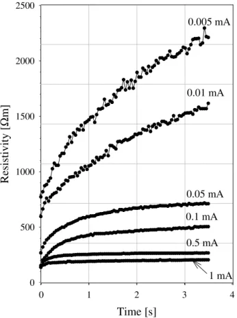
Fig. 2.Calculated resistivity of sandstone sample 226A for different amplitude of applied current.
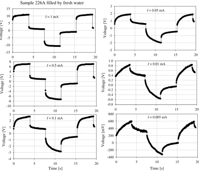
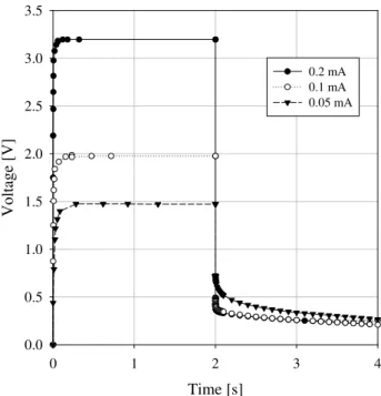
containing straight half limited capillaries does not depend on structural and physical properties of pores and pores’ elec-trolyte. This model is not common in real structures of in-terlaced pores in sediments. Also let us note regardless of mentioned unequal transport properties in case of membrane polarization the Eqs. (1) and (2) do not contain the most im-portant parameters of current flow in pores’ system – transfer numbers. However this model as well as equivalent electrical circuit models has been widely used to describe electrode po-larization parameters and has resulted in two important con-clusions being made which have been accepted by all geo-physicists, namely: 1. Processes of IP at time on and time off are the same. 2. There is a linear dependence between applied electrical current and IP amplitude. Practically all existing instruments register transient decay during time-off. Physical modelling has been performed at the CGS for several years using the instrument RIP built by M. Hauger. However, the results of laboratory measurements very often show the opposite. Figure 1 demonstrates the result of labo-ratory measurements of sample of sandstone number 226A.
A constant current pulse train is generated in the transmit-ter and passed through the sample via the current electrodes in the sample holder .The porosity of sample is 16%. The
Applied current [mA]
0.001 0.01 0.1 1
C
h
ar
g
eb
il
it
y
[
%
]
0 20 40 60 80 100
Fig. 3.Measured chargeability vs. applied current. Sample 226A.
measurements were performed for different electrical cur-rents (from 0.05 mA to 1 mA). The voltage is measured at the electrodes connected to the sample. The measured volt-age shows no linear dependence on applied current. Since the geometrical shape of the sample is known, resistivity can be calculated as follows:
ρ= V I
S
L (3)
whereV is the voltage,I is constant current setting,Sis the surface area of sample, and L is the sample length. Figure 2 demonstrates calculated resistivity of sample for different amplitude of applied current. Obviously the measured resis-tivity of sample depending on current and that phenomenon does not suit the Ohm’s law.
Moreover the Fig. 3 demonstrate the value of chargeability measured by different current and calculated asη=V0.5/Vd, whereV05 is a voltage measured at the time 0.5 s andVdis a primary voltage. This figure demonstrates that the charge-ability also depends on the magnitude of the applied current and increases when current decreases.
Fig. 4.Model of three connected capillaries.
layers could touch each other and act as a barrier to anions. Under the influence of an electric field a varying concentra-tion of anions and caconcentra-tions result. This behaviour can be de-scribed as passive and active sections where the notation “ac-tive” and “passive” refers to the polarization origin within the porous rocks.” This type of polarization is mentioned in the book by J. Sch¨on as polarization by constrictivity of pores. However this kind of polarization hardly ever develops. We mentioned already Marshal and Madden (1959). These au-thors as well as Kobranova (1986) showed that this type of polarization occurs in sediments containing pores with differ-ent surface areas in which the mobilities of ions and transfer numbers are different. They also showed that when electrical current flows through a channel containing pores with dif-ferent radii (transfer numbers), an excess/loss of ions accu-mulates at the boundaries. Marshal and Madden (1959) pre-sented the equation of steady-state conditions conductance (with our symbols) as:
σdc=
FMiku0
1 n2k +
A B
1 n1k
l1
hn
1k n1a 1+
A B
+n2kc n2a 1+
A B
i (4)
where A=l1/ l2 B=D1n/D2n, l1 l2 are length of large (1) and narrow (2) capillaries, respectively, D is a diffu-sion coefficient, u0 is net concentration of free solution, n2k, n1k n2a, n1aare transfer numbers of cations and an-ions in narrow and large capillaries. Subscriptskanda indi-cate cations and anions respectively, numerical subscript in-dicate the number of pores (1, 2) respectively. However the authors did not analyze when steady-state condition occurs and physical phenomena and mathematical consideration ex-plaining this condition. We can only refer to Pape and his co-authors (1987). They tried to adjust an electrical circuit as well as fractal model to describe processes causing by con-strictivity of pores. Some aspects of this kind of polarization were discussed by Titov et al. (2002).
This paper intends to develop the model of polarization by constrictivity of pores by giving briefly a mathematical con-sideration of the process and discusses the physical phenom-ena occurring during time-on and time-off of applied
electri-Time [s]
0.00 0.05 0.10 0.15 0.20 0.25 0.30
E
lec
tr
il
y
te
co
n
cen
tr
at
io
n
[
m
o
l/
l]
0.000 0.002 0.004 0.006 0.008 0.010
Fig. 5.Boundary conditions in the pores. Sample contains numer-ous pore configurations.
cal current. Therefore we shall also name this kind of polar-ization as membrane polarpolar-ization because the origin of this process is to form membranes between connected pores.
2 Theoretical consideration
The complete theoretical consideration of membrane polar-ization caused by constrictivity of pore radii was developed and published (Zadorozhnaya and Hauger, 2007, 2008a, b). Here we mention only the solutions of the mathematical problems and discuss the most important obtained results.
The duration of the polarization process in pores is con-trolled by the transfer numbers, radii of the connected pores, and amplitude of the electrical current. If a large pore con-nects to a narrow pore, the ion concentration in the vicinity of the contact decreases. Our aim is to provide modelling of membrane polarization in rocks with complex structures of pore spaces and prove the issues mentioned above. The primary model (cell) consists of three connected pores with surface areasS1(central pore),S2andS3are respectively left and right pores (Fig. 4). Afterwards more complicated mod-els containing many connected pores of different sizes and transfer numbers are submitted. The solutions are presented for time-on and time-off. Then we also intend to show that the resistivity of sediments change during the application of an electrical current.
Table 1.Parameters of model.
r1[mm] r2[mm] r3[mm] n1k n2k n3k
Model 1 4.0e-5 1.0e-5 1.4e-5 0.798 0.949 0.976
Model 2 1.0e-5 1.4e-5 4.0e-5 0.949 0.976 0.798
Model 3 1.4e-5 1.0e-5 4.0e-5 0.976 0.949 0.798
Model 4 1.4.e-5 4.0e-5 1.0e-5 0.976 0.798 0.949
this case (Koshlyakov et al., 1970). The general diffusion equation is the following:
∂u ∂t =a
2∂2u
∂x2 (5)
Whereuis the salinity of the solution,a2=Dis a diffusion coefficient. The boundary conditions and initial conditions are:
u|x=0=ψ1(t ), u|x=l =ψ2(t )andu|t=0=ϕon(x), (6) wherelis the length of the central pore 1,ϕon(t )is constant and equal to the salinity of cations and anions at steady con-dition. It was shown (Zadorozhnaya and Hauger, 2007) that the boundary conditions can be written as follows:
u|t=0=u0k+u0a=ϕon(x), u0k=u0a=u0/2 (7)
u|x=0 =u0k+u12k(t )+u0a+u12a(t )=ψ1(t ),
u|x=l =u0k+u13k(t )+u0a+u13a(t )=ψ2(t ), (8) where
u12k(t )=
I2Mkt F zDS1S2σk
(n2k−n1k),
u13k(t )=
I2Mkt F zDS1S2σk
(n1k−n3k)
u12a(t )=
I2Mkt F zDS1S2σa
(n1a−n2a),
u13a(t )=
I2Mat F zDS1S2σa
(n3a−n1a). (9)
Here numerical subscript indicate the number of pores (1, 2 and 3),u0 is the initial salinity of the solution,u1 is the excess of salinity at the boundary between pores, σis the conductivity of ions,nis the transfer number of ions in the pore,I is an electrical current flowing in the pore,t is time. Equation (8) show a linear dependency of salinity on time at the boundaries between capillaries and depends on the square value of the electrical currentI. Obviously ifn2=n1and/or n3=n1there is not an excess of ions on the contacts between pores. On the other hand if pore radii are different but both are large the influence of the double electrical layers (DEL) can be neglected becausen2=n1=0.5 and/orn3=n1=0.5 and no excess of ions occurs at the boundaries.
Table 2.Model of sample consisting 12 cells.
Number of cells r1 r2 r3 l1 n
1 1.3e-6 1.2e-8 1.4e-8 9.5e-4 50
2 1.1e-6 2.0e-8 2.0e-8 8.5e-4 20
3 1.15e-6 1.3e-8 1.4e-8 6.4e-4 50
4 6.5e-7 1.3e-8 1.4e-8 6.4e-4 75
5 5.0e-7 1.2e-8 2.0e-8 5.5e-4 100
6 4.0e-7 1.7e-8 1.8e-8 4.7e-4 175
7 3.0e-7 1.5e-8 1.6e-8 4.0e-4 200
8 2.0e-7 1.5e-8 1.5e-8 3.5e-4 250
9 1.7e-7 1.6e-8 1.6e-8 4.4e-4 200
10 1.5e-7 1.8e-8 1.6e-8 3.5e-4 200
11 1.3e-7 0.8e-8 1.6e-8 1.7e-4 200
12 1.2e-7 1.5e-8 1.3e-8 1.0e-4 250
The solution of (5) can be found as the following series:
u(x, t )= ∞
X
n=1
Tn(t )·sinnπ x
l , (10)
If ϕon=const than ψ1(t )−(−1)nψ2(t )=Y+X·t, where X=(K12−(−1)nK31),
Y = u0(1−(−1))n
,
K12k =
I2Mkt F zDS1S2σk
(n2k−n1k),
K12a=
I2Mk F zDS1S2σa
(n1a−n2a)
K31k =
I2Mk F zDS1S2σk
(n1k−n3k),
K31a=
I2Mat F zDS1S2σa
(n1a−n2a).
The solution of (5) with boundary conditions (6) can be written as (Zadorozhnaya and Hauger 2007):
Tn(t )=Cnexp(−At )+ 2nπ a2
l2
X
t
A−
1 A2
+exp(−At )
X
A2− Y A
+YA
. (11)
Distance along the pore [mm]
0.0 0.2 0.4 0.6 0.8 1.0
E
lect
ro
ly
te
co
n
ce
n
tr
at
io
n
[m
o
l/
l]
0.000 0.005 0.010 0.015 0.020 0.025 0.030 0.035
t = 0.5 s t = 1.2 s t0 = 2.2 s MODEL 1
a
Distance along the pore [mm]
0.0 0.2 0.4 0.6 0.8 1.0
C
o
n
cen
tr
at
io
n
o
f
el
ect
ro
ly
te
[m
o
l/
l]
0.000 0.002 0.004 0.006 0.008 0.010 0.012 0.014 0.016 0.018 0.020
t = 0.2 s t = 0.4 s t0 = 079s
MODEL 2
b
Distance along the pore [mm]
0.0 0.2 0.4 0.6 0.8 1.0
C
o
n
cen
tr
at
io
n
o
f
el
ect
ro
ly
te
[m
o
l/
l]
0.008 0.010 0.012 0.014 0.016 0.018 0.020
t = 0.2 s t = 0.4 s t = 0.8 s MODEL 3
c
Distance along the pore [mm]
0.0 0.2 0.4 0.6 0.8 1.0
C
o
n
ce
n
tr
at
io
n
o
f
el
ect
ro
ly
te
[m
o
l/
l]
0.000 0.002 0.004 0.006 0.008 0.010 0.012
t = 0.2 s t = 0.4 s t0 = 0.792 s
MODEL 4
d
Distance along the pores [mm]
0.25 0.30 0.35 0.40 0.45
E
lect
ro
ly
te
co
n
ce
n
tr
at
io
n
[
m
o
l/
l]
0.000 0.002 0.004 0.006 0.008 0.010 0.012 0.014 0.016 0.018
Initial concentration ϕ(x)
t= 0.0005 s t= 0.005 s t= 0.05 s t= 0.00005 s
t= 0.1 s
a
Distnce along the pore [mm]
0.25 0.30 0.35 0.40 0.45
E
le
ct
ro
ly
te
co
n
cen
tr
at
io
n
[
m
o
l/
l]
0.000 0.002 0.004 0.006 0.008 0.010 0.012 0.014 0.016 0.018
1
2
b
Fig. 7. Model 1. Electrolyte concentration distribution during the time off at selected times. Time of blockaget0=0.0158(a). Com-parison of electrolyte concentration distribution at time on (curve 1) and time off (curve 2) at fixed time 0.0158 s(b).
t0as the critical time of the polarization process. Thent0is equal to:
t0= −
u0kF zDS1S2σk I2M
k(n1k−n3k)
. (12)
Now we come to an important conclusion: the duration of the polarization processt0 in pores is controlled by the transfer numbers and radii of the connected pores. So the boundary conditions (9) for our problem exist up to timet0, after which the electrical circuit ruptures and the potential difference between the pore ends becomes constant.
Figure 5 demonstrates left boundary conditions (between capillaries 1 and 3) for a sample containing ten pore cells. Why are boundary conditions not linear? They remain lin-ear until a pore blockage occurs, then the current finds suit-able unblocked pores and continues flowing through these un-blocked pores until another blockage occurs.
Time [s]
0 1 2 3 4
V
o
lt
ag
e
[
V
]
0.0 0.5 1.0 1.5 2.0 2.5 3.0 3.5
0.2 mA 0.1 mA 0.05 mA
Fig. 8.Mathematical simulation: voltage vs time for different am-plitude of electrical current. 12 cell’s model.
Time [s]
0.0 0.5 1.0 1.5 2.0
R
es
is
ti
v
it
y
[
Ω
m
]
0 200 400 600 800 1000
I = 0.05 mA
I = 0.1 mA
I = 0.2 mA
Density [g/cm3]
1.8 2.0 2.2 2.4 2.6 2.8
C
h
ar
g
eab
il
it
y
[
%
]
0 5 10 15 20 25 30
Fig. 10.Cargeability of of samples of kimberlite vs they density.
Porosity [%]
0 10 20 30 40 50
C
h
ar
g
ea
b
il
it
y
[
%
]
0 10 20 30 40 50
Fig. 11. Mathematical simulation: Chargeability vs porosity of sample.
Calculation of a concentration distribution occurring in the capillaries at time-off is more complicated and is presented as two successful approximations. First approximation:
– Concentration distribution in the pore 1 (Problem of free exchange of ions with host media);
– Numerical boundary conditions following from concen-tration leveling in pore1;
– Calculation of boundary conditions for surrounding pores (using general equation for unlimited tube);
Time [s]
0 1 2 3 4
V
o
lt
a
g
e
[V
]
0.0 0.5 1.0 1.5 2.0 2.5 3.0
0.10 %
0.15 % 0.25 %
0.35 %
Fig. 12.Mathematical simulation: voltage vs porosity of sample.
– Concentration distribution in connected pores (Diffu-sion equation for half limited pore with specified bound-ary and initial conditions).
Second approximation:
– Additional concentration along the pores due to sources of ions at the contacts of pores. (Inhomogeneous diffu-sion equation where source functions are found as the difference between boundary conditions defined at dif-ferent sides of connected pores (zero initial conditions). The calculation showed that after time-off the diffusion process slowly leveled the concentration along the pores reaching the initial concentration.
The boundary and initial conditions of diffusion Eq. (5) are different at time-on and time-off. Consequently the so-lutions of Eq. (5) for the time-on and time-off are different. Obviously potential and potential differences occurring be-tween two electrodes are also different for both time-on and time-off.
If current is flowing through the sample containing numer-ous pore configurations the potential can be presented as a sum of potentials that occur due to flowing conductive cur-rentUcurr(t )and excess concentrationUexcess(t )at the con-tacts:
Uswitch on(t )=Ucurr(t )+Uexcess(t ) (13) If electrical current does not flow through the sample the potential is defined by excess of concentration Uexcess (t ) only. Then:
Density [g/cm3]
1.8 2.0 2.2 2.4 2.6 2.8
R
es
is
ri
v
it
y
[
Ω
m
]
10 100 1000 10000
Fig. 13.Resistivity of samples of kimberlyte vs density.
3 Analyze and discussion
3.1 Mathematical simulation of salinity distribution along the pores
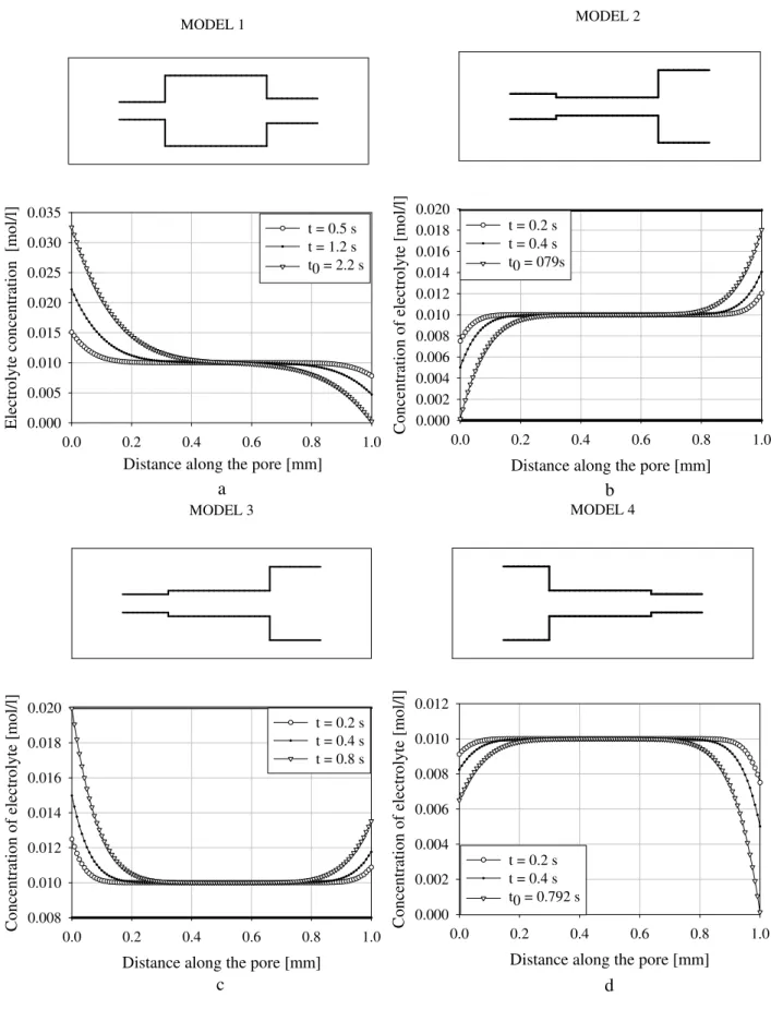
The computing programs have been written in Mat lab and results of calculations have to be discussed now. For cal-culations four types of models (Fig. 6a, b, c, d) were used. Parameters of models are shown in the Table 1. Length of main pore is always equal to 1 mm; electrolyte concentration is 0.01 mol/l. The direction of current flow as shown in the Fig. 4.
Figure 6a, b, c, d demonstrate salinity distribution in dif-ferent types of model for the time-on. If a large capillary is connected to a narrow capillary the difference of trans-fer numbers is negative and a decrease of ion concentration occurs (Fig. 6a, b, c). The duration of the polarization pro-cess depends on the pore radii and transfer numbers. Time of blockage is much earlier in model 2 and model 4 (Fig. 6b, d) (0.79 c) but 2.2 c in model 1 (Fig. 6a). Model 3 (Fig. 6c) will never be blocked since the concentration of ions in model 4 decrease at both ends of the main pore.
3.2 Difference at time-on and time-off
Figure 7a demonstrates the electrolyte concentration distri-bution during the time off at selected times in model 1. Time of blockage in this model is equal tot0=0.0158 c. The diffu-sion process slowly leveled the concentration along the pores reaching the initial concentration 0.01 mol/l.
Figure 7b demonstrates the comparison of electrolyte con-centration distribution at the same fixed time for time-on and time-off for model 1. As mentioned above if electrical
cur-Concentration of electrolyte [mol/l]
0.001 0.01 0.1 1
T
im
e
o
f
b
lo
ck
ag
e
[s
]
0.0001 0.001 0.01 0.1 1 10 100 1000 10000
Fig. 14. Time of blockage vs electrolyte concentration. Pore radii: r1=9.75e-8m,r3=6.25e-8m.
Distance along the cell [m]
0.0045 0.0050 0.0055 0.0060 0.0065
C
o
n
ce
n
tr
at
io
n
(
n
o
rm
al
iz
ed
)
C
/C
0
0 2 4 6 8 10
3e-1 2e-1 1e-1
7e-2
5e-2 3e-2
1e-2 1e-3
Fig. 15. Concentration distribution along the cell at selected time (1 s or less) for different electrolyte concentration.
rent will be applied to this model then blockage of pores’ channel occurs at the time 0.0158 s a. However at the same time after time-on of electrical current the ions are neither leveled completely nor even leveled considerably (Fig. 7b). Obviously the process of diffusion is much slower than con-centration distribution due to applied current (time-on). This fact has been proved by a large number of measurements done by Hauger in CGS (see Fig. 12 as example).
3.3 Voltage and electrical current
0 5 10 15 20
V
o
lt
a
g
e
[V
]
-10 -8 -6 -4 -2 0 2 4 6 8 10
I = 0.5 mA
Time [s]
0 5 10 15 20
V
o
lt
ag
e
[V
]
-1.5 -1.0 -0.5 0.0 0.5 1.0 1.5
I = 0.1 mA
V
o
lt
ag
e
[V
]
-0.8 -0.6 -0.4 -0.2 0.0 0.2 0.4 0.6 0.8
I = 0.05 mA
V
o
lt
ag
e
[V
]
-0.15 -0.10 -0.05 0.00 0.05 0.10 0.15 0.20
I = 0.01 mA
0 5 10 15 20
V
o
lt
ag
e
[
m
V
]
-80 -60 -40 -20 0 20 40 60 80
I = 0.005 mA
Time [s]
0 5 10 15 20
V
o
lt
ag
e
[m
V
]
-15 -10 -5 0 5 10 15
I = 0.001 mA
Fig. 16.Laboratory measurements of sandstone 261C filled by salty water.
follows from boundary conditions (9), which are having cur-rent, squared (I2). Let us analyze mathematical simulation of IP effect depending on current. Usually rocks contain numerous numbers of pore configurations and blockage of pores occurs all the time for the duration of current flow. Let us select petrophysical model consisting of 12 types of cells (Table 2). The ratio of cells with different surface ar-eas (source of IP effect) and straight capillaries where IP ef-fect does not occur is 0.117, it means 11.7% of capillaries have surface areas and transfer numbers different for con-nected pores. Mathematical simulations (Fig. 8) confirmed results obtained by laboratory measurements namely voltage increases vs. increasing current. However there is no linear dependence between both parameters. Why does this occur? If current is big enough then blockage of pores occurs at the earlier times. In this case ions blocked capillaries are located very close to the contacts and the amount of ions involved into this process is very small. So the contribution ofUexcess
is very small and voltage is defined by conductivity current Ucurr. When time of blockage occurs later the amount of ions involved with the polarization process increases (see Fig. 7a) and the ratio betweenUcurrandUexcessincreases as well. In this case the resistivity of sample also increases (Fig. 9).
Time [s]
0 1 2 3 4
R
es
is
tiv
ity
[
Ω
m
]
200 220 240 260 280 300 320 340
0.5 mA
0.001 mA 0.005 mA 0.01 mA 0.05 mA
0.1 mA
Fig. 17. Calculated resistivity of sandstone sample 261C filled by salty water for different amplitude of applied current.
3.4 Porosity
It is well known that resistivity decreases with porosity. The laboratory measurements of samples of kimberlite collected from different depths have been used. Unfortunately param-eters of porosity had not been measured during the experi-ments but only density. However usually rocks with low den-sity are characterized by higher poroden-sity. All measurements were measured with the same amplitude of current (0.5 mA). The Fig. 10 demonstrates measured chargeability of kimber-lites of different density. Obviously chargeability decreases vs. density; it means we can suppose the chargeability is in-creasing with porosity.
Figure 11 shows calculated chargeability of models (Ta-ble 2) with different porosity. The same dependence has been observed: increasing porosity follows increasing chargeabil-ity. The explanation of physical phenomenon is the same. High porous rocks involve more ions to induced polarization process than low porous rocks. Process of leveling is slow and as denser clouds of ions concentrate at the contact the longer is the following process of leveling.
Figure 12 shows mathematical modeling of voltage of samples with different porosity. However this dependence is more complicated. In low porous rocks the voltage (resistiv-ity) decreases with decreasing porosity. However as porosity increases so does the amount of ions involved in IP effect and the dependence becomes reversed: increasing porosity results in increasing voltage (resistivity). In this caseUexcess is to be dominated byUcurr.
I
= 0.5 mA
Time [s]
0 2 4 6 8
V
o
lt
a
g
e
[V
]
0 2 4 6 8
a
I
= 0.1 mV
Time [s]
0 2 4 6 8
V
o
lt
a
g
e
[V
]
0.0 0.5 1.0 1.5 2.0 2.5 3.0 3.5
b
I
= 0.05 mA
Time [s]
0 2 4 6 8
V
o
lt
a
g
e
[V
]
0.0 0.5 1.0 1.5 2.0 2.5
c
Table 3.Model of sample 226A containing 22 cells.
Number Radius of Radius of Radius of Length of Number of of cells left porer2 main porer1 right porer3 main porel1 cells in the
sample
1 1.3e-5 2.5e-2 1.3e-5 1.67e-2 3870
2 1.4e-5 1.18e-2 1.4e-5 2.00e-2 14180
3 1.4e-5 6.67e-3 1.4e-5 2.00e-2 64440
4 1.4e-5 4.74e-3 1.4e-5 2.17e-2 97950
5 1.4e-5 3.85e-3 1.4e-5 2.00e-2 28300
6 1.4e-5 2.95e-3 1.4e-5 2.00e-2 28300
7 1.3e-5 2.88e-3 1.4e-5 1.72e-2 270700
8 1.3e-5 2.82e-3 1.4e-5 1.47e-2 322200
9 1.3e-5 2.69e-3 1.4e-5 1.33e-2 309300
10 1.3e-5 2.24e-3 1.4e-5 1.33e-2 451100
11 1.3e-5 1.92e-3 1.4e-5 1.27e-2 773300
12 1.3e-5 1.73e-3 1.4e-5 1.20e-2 902200
13 1.3e-5 1.47e-3 1.3e-5 1.17e-2 1288800
14 1.4e-5 1.40e-3 1.4e-5 1.17e-2 1353300
15 1.4e-5 1.28e-3 1.4e-5 1.17e-2 1288800
16 1.3e-5 1.09e-3 1.4e-5 1.17e-2 1417700
17 1.3e-5 9.0e-4 1.4e-5 1.17e-2 1675400
18 1.3e-5 8.7e-4 1.4e-5 1.17e-2 1933200
19 1.4e-5 7.9e-4 1.4e-5 1.17e-2 2577600
20 1.4e-5 7.1e-4 1.4e-5 1.17e-2 2964300
21 1.4e-5 6.4e-4 1.4e-5 1.17e-2 3479800
22 1.4e-5 5.8e-4 1.4e-5 1.17e-2 3866400
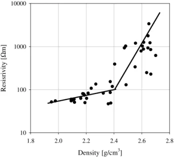
The following dependence presented in semi-logarithm scale can be seen in the Fig. 13. The resistivity of kimberlites decreases very fast from 4000 to 100 Ohmm with decreas-ing density (i.e. increasdecreas-ing porosity) from 2.8 to 2.6 g/cm3. However resistivity of low dense (higher porous) rocks re-mains more or less stable (approximately 80–100 Ohmm) with further decreasing density from 2.0 to 1.95 g/cm3. So this example (laboratory measurements and mathematical modeling of resistivity of porous rocks) demonstrates a very complicated relationship between resistivity and porosity of rocks.
3.5 Electrolyte concentration
It is known that all kinds of polarization effects exist only if concentration of electrolyte filled pores space of rocks is low. Let us see a mechanism of membrane polarization ef-fect depending on this parameter. The Eq. (12) shows that the time taken to block the pores is linearly dependent on the conductivity of electrolyteσ. The Fig. 14 demonstrates dependencet0on concentration of electrolyte in a single pores cell with following parametersr1=9.75e-8m and r3 =6.75e-8m,I=13e-13A. The time of pore blockage is linearly de-pendant on electrolyte concentrationu, and transfer number difference decreases. So ifu=0.001 mol/l (0.056 g/l for NaCl solution, fresh, drinking water) when time of blockage
oc-curs at the time 3.82e-4s. Ifu=0.1 mol/l (5.6 g/l, salty water), when time of blockage occurs at the time 8.5 s. Ifu=1 mol/l (56 g/l, concentrated solution), when time of blockage occurs at the time 3204 s. It means the process of concentration of ions in the vicinity of contracted pores with different surface areas becomes slower with increasing concentration of elec-trolyte.
0.0 1.0 2.0 3.0 4.0 5.0 6.0 7.0 8.0 9.0 1.66 E-07 1.39 E-07 1.17 E-07 1.12 E-07 1.05 E-07 9.41 E-08 8.79 E-08 7.17 E-08 5.51 E-08 4.99 E-08 4.84 E-08
Volume of pore [mm3]
R el at iv e v o lu m e o f la rg e sh ap ed p o re s [% ] a 0.0 1.0 2.0 3.0 4.0 5.0 6.0 7.0 8.0 9.0
0.0E+00 5.0E-08 1.0E-07 1.5E-07 2.0E-07
Volume of pore [mm3]
R el at iv e v o lu m e o f la rg e sh ap ed p o re s [% ] b 0.0 1.0 2.0 3.0 4.0 5.0 6.0 7.0 8.0 9.0 8.18 E+00 6.82 E+00 5.75 E+00 5.52 E+00 5.17 E+00 4.63 E+00 4.32 E+00 3.53 E+00 2.71 E+00 2.45 E+00 2.38 E+00
Pore radius [mm]
R el at iv e v o lu m e o f la rg e s h a p ed p o re s [% ]
c
Fig. 19. Pore size distribution of sample 226A.(a)Histogram showing relative volume of cylindrical shaped pores vs. their volume. (b)
Relative volume of cylindrical shaped pores vs. their volume;(c)Histogram showing relative volume of cylindrical shaped pores vs. their pore radiusr1.
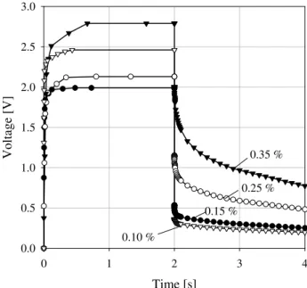
The Fig. 16 demonstrates the measured voltage of a sam-ple of sandstone number 261C, filled by salty water (con-centration 7 g/l or 0.125 mol/l). If applied current is high enough the IP effect can be recognized due to earlier block-age of pores. Decreasing current follows linear dependence voltage on current – no IP effect can be observed.
influence on the value of resistivity of sample (∼250 Ohmm). These laboratory measurements confirmed our theoretical consideration.
3.6 Frequency
The laboratory measurements and mathematical modeling (as example Fig. 7a time-on case and 7a – time-off) show that the process of membrane IP is relatively slow. Which is why there is no IP effect with high frequency of applied current: In fact the process of IP may not even have started during the short current cycle.
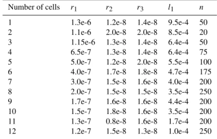
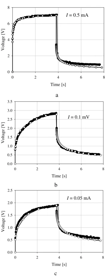
3.7 Testing the theory with laboratory measurements Now we must reconcile the theory and laboratory measure-ments. Figure 18a, b, c demonstrate mathematical modeling of the IP effect for different applied currents, namely 0.5 mA, 0.1 mA and 0.05 mA (time-on) and the subsequent diffu-sion process (time-off). These figures show calculated pores structure models for sample 226A. These figures demon-strate the possible size distribution of pores in the sample. The parameters of pores are shown in the Table 3, 22 cells of pores can roughly describe the pores structure of this sample. Figure 19a presents a histogram of the relative volume of cylindrical shaped poresVi/V6in the sample (whereVi is the volume of all main pores ofi-size and V6 is the total volume of cylindrical shaped pores) vs. their volume. Obvi-ously the large pores occupy more space but the number of these pores are relatively small (Table 3). The relationship between the relative amount of shaped pores and their vol-ume is linear for this model (Fig. 19b). Another histogram (Fig. 19c) shows the relative amount of cylindrical shaped pores vs. their pore radiusr1. This is the first attempt to calculate the pore size distribution using IP laboratory data. Using different currents allow us to obtain more reliable data. However this approach must be continued and enhanced by further study. Agreement between the calculation results and laboratory data is good. Some differences at time-off for a large current can be explained by the limited numbers of pore cells especially of small scale.
We foresee a comparison between the pore size distribu-tion obtained from the interpretadistribu-tion of laboratory measure-ments, and those obtained using neutron tomography which allows for the scanning of samples with a minimum spatial resolution of 100µm (De Beer et al., 2007).
4 Conclusions
Mathematical modeling of a little known model of IP re-ferred to as “induced polarization caused by constrictivity of pores” was developed. Polarization occurs in all types of rocks if surface areas and transfer numbers are different for connected pores. The duration of the polarization process
depends on two parameters: pore radii of connected capil-laries and transfer numbers. During the polarization process all contacts between pores of different transfer numbers will be blocked and the electrical current will flow through the remaining canals. Two phenomena control the amplitude of potential difference at time-on: 1. Successive blockage of pores increases the resistivity of sediments and results in increased measured potential difference. 2. Excess concen-tration of electrolyte at the boundaries between pores with different radii provides an additional potential. The ampli-tude of the potential difference (voltage) of such rocks not only depends on solutions filling pore spaces, porosity and tourtuosity of pores channels, but also on ion mobility, diffu-sion coefficient, and difference of transfer numbers. During time-on a voltage is occurred due to flowing currentUcurr(t ) and excess concentrationUexcess(t )at the contacts. However during the time-off only the excess of concentrationUexcess (t )is involved in the diffusion process which intends to level the ion concentration along the pores. It was shown that mea-sured chargeability is proportional to porosity. Blockage of pores and excess/loss ions at the contacted pores control this physical parameter. However the relationship between resis-tivity and porosity is very complicated. Mathematical mod-eling and laboratory measurements both confirmed the mem-brane IP effect diminishing with increasing salinity of fluid filled pores of rocks. The model of IP caused by constrictiv-ity of pores can be regarded as a general model for membrane polarization. The new algorithm was tested on laboratory measurements data showing its good agreement with theory. The first attempt to calculate pore size distribution using IP laboratory data has been presented.
Membrane polarization does not exist on high frequency of electrical current. Which is why resistivity measured by direct and alternating current are different. The definition of the membrane IP effect is: “Membrane IP is the successive blockage of inter-pore connections due to the excess distri-bution of ions during current flow”.
Acknowledgements. The author thanks M. E. Hauger for laboratory measurements and productive discussions.
Edited by: L. V. Eppelbaum
Reviewed by: three anonymous referees
References
Anderson, L. A. and Keller, G. V.: A study in induced polarization, Geophysics, 24(5), 848–864, 1964.
De beer, F., Zadorozhnaya, V., Middleton, M., and Schoeman, C.: Neutron imaging in South Africa adds value to geosciences and petrophysics, 19th geophysical conference and exhibition, Perth, Western Australia, 18–22, 2007.
Keller, G. V. and Licastro, P. H.: Dielectric constant and electrical resistivity of natural state cores, US Geol. Survey Bull., 1052, 257–285, 1959.
Jost, W.: Diffusion in Solids, Liquids, Gases: New York, Academic Press, Inc., 558 p., 1952.
Kobranova, V. N.: Petrophysics, Nedra, Moscow, 392 p., 1986, in Russian.
Koshlyakov, N. S., Gliner, E. B., and Smirnov, M. M.: Partial Differentiation of Equations in Mathematical Physics, Vysshaya shkola., Moscow, 710 p., 1970, in Russian.
Marshal, D. J. and Madden, T. R.: Induced Polarization, a Study of its cases, Geophysics, 24(4), 790–816, 1959.
Pipe, H., Riere, L., and Schopper, J. R.: Theory of semi-similar network structures in sedimentary and igneous rocks and their investigations with microscopical and physical methods, J. Mi-croscopy, 2, 121–147, 1987.
Sch¨on, J.: Physical Properties of Rocks. Fundamental and Prin-ciples of Petrophysics. Handbook of Geophysical Exploration. Seismic Exploration, Volume 18, New York, Pergamon, Press, Inc., 583 p., ISBN 0 08 0410081, 1996.
Titiov, K., Komarov, V., Tarasov, V., and Levitski, A.: Theoretical and experimental study of time domain-induced polarization in water saturated sands, J. Appl. Geophys., 50, 417–433, 2002. Ward, S.: Resistivity and Induced Polarization Methods, in:
Geotechnical and environmental geophysics, Investigation in Geophysics, No. 5, edited by: Ward, S., SEG, 169–189, 1990. Zadorozhnaya, V. Y. and Hauger, M. E.: Membrane polarization
on rocks and measured resistivity, in: Earth Elecrtomagnetic In-vestigations, edited by: Spichak, V. V., III International School-Seminar on Electromagnetic Sounding of the Earth (EMS-2007), Moscow, Russia, Lecture, 149–167, 2007.
Zadorozhnaya, V. Y. and Hauger, M. E.: Mathematic simulation of the membrane polarization occurring in rocks due to applied electrical current, Physics of the Solid Earth, in press, 2008a. Zadorozhnaya V. Y. and Hauger, M. E.: Polarization processes in