Assessment of the indirect calibration of a rainfall-runoff model for ungauged catchments in Flanders

(1)

HESSD

10, 103–144, 2013

Assessment of indirect calibration

N. De Vleeschouwer and V. R. N. Pauwels

Title Page

Abstract Introduction

Conclusions References

Tables Figures

◭ ◮

Back Close

Full Screen / Esc

Printer-friendly Version Interactive Discussion

Discussion

P

a

per

|

Dis

cussion

P

a

per

|

Discussion

P

a

per

|

Discussio

n

P

a

per

|

Hydrol. Earth Syst. Sci. Discuss., 10, 103–144, 2013 www.hydrol-earth-syst-sci-discuss.net/10/103/2013/ doi:10.5194/hessd-10-103-2013

Hydrology and Earth System Sciences Discussions

This discussion paper is/has been under review for the journal Hydrology and Earth System Sciences (HESS). Please refer to the corresponding final paper in HESS if available.

Assessment of the indirect calibration of

a rainfall-runo

_ff

model for ungauged

catchments in Flanders

N. De Vleeschouwer1and V. R. N. Pauwels2

1

Laboratory of Hydrology and Water Management, Ghent University, Ghent, Belgium

2

Department of Civil Engineering, Monash University, Clayton, Victoria, Australia

Received: 29 November 2012 – Accepted: 11 December 2012 – Published: 7 January 2013 Correspondence to: N. De Vleeschouwer (niels.devleeschouwer@ugent.be)

(2)

HESSD

10, 103–144, 2013

Title Page

Tables Figures

◭ ◮

Back Close

Full Screen / Esc

Discussion

P

a

per

|

Dis

cussion

P

a

per

|

Discussion

P

a

per

|

Discussio

n

P

a

per

|

Abstract

In this paper the potential of discharge-based indirect calibration of the Probability Dis-tributed Model (PDM), a lumped rainfall-runoff(RR) model, is examined for six selected catchments in Flanders. The concept of indirect calibration indicates that one has to es-timate the calibration data because the catchment is ungauged. A first case in which in-5

direct calibration is applied is that of spatial gauging divergence: Because no observed discharge records are available at the outlet of the ungauged catchment, the calibration is carried out based on a rescaled discharge time series of a very similar donor catch-ment. Both a calibration in the time domain and the frequency domain (a.k.a. spectral domain) are carried out. Furterhermore, the case of temporal gauging divergence is 10

considered: Limited (e.g. historical or very recent) discharge records are available at the outlet of the ungauged catchment. Additionally, no time overlap exists between the forcing and discharge records. Therefore, only an indirect spectral calibration can be performed in this case. To conclude also the combination case of spatio-temporal gauging divergence is considered. In this last case only limited discharge records are 15

available at the outlet of a donor catchment. Again the forcing and discharge records are not contemporaneous which only makes feasible an indirect spectral calibration. The modelled discharge time series are found to be acceptable in all three considered cases. In the case of spatial gauging divergence, indirect temporal calibration results in a slightly better model performance than indirect spectral calibration. Furthermore, 20

indirect spectral calibration in the case of temporal gauging divergence leads to a bet-ter model performance than indirect spectral calibration in the case of spatial gauging divergence. Finally, the combination of spatial and temporal gauging divergence does not necessarily lead to a worse model performance compared to the separate cases of spatial and temporal gauging divergence.

(3)

HESSD

10, 103–144, 2013

Title Page

Tables Figures

◭ ◮

Back Close

Full Screen / Esc

Discussion

P

a

per

|

Dis

cussion

P

a

per

|

Discussion

P

a

per

|

Discussio

n

P

a

per

|

1 Introduction

The practical application of RR models requires a proper assignment of the param-eter values, also known as the process of parametrisation or calibration (Duan et al., 1992). Ideally, this calibration process should be fed by in situ measurements or remote sensing data. Practical considerations, however, implicate an alternative strategy. In 5

a classic calibration framework the parameter values are adjusted until the match be-tween the modelled and observed output (e.g. discharge) is found to be acceptable. As hydrologic models increasingly become more sophisticated, the iterative parameter adjustments are usually performed by specific optimalisation algorithms. Commonly used algorithms in hydrologic modelling are e.g. genetic algorithms (Reed et al., 2000) 10

like the Shuffled Complex Evolution Algorithm (SCE-UA) (Duan et al., 1992), local and multistart simplex methods (Gan and Biftu, 1996), Particle Swarm Optimisation (PSO) (Kennedy and Eberhart, 1995; Scheerlinck et al., 2009), Simulated Annealing (SA) (Thyer et al., 1999), etc. In practice the conditions to perform an ordinary direct cali-bration are not always fulfilled. This implies an indirect calicali-bration strategy. In the past 15

decade, the research concerning indirect calibration has gained attention in the hydro-logic community through the Prediction in Ungauged Basins (PUB) initiative (Sivapalan et al., 2003) set up by the International Association of Hydrological Sciences (IAHS). In scarcely gauged regions, discharge records may lack entirely for the catchment of inter-est, and may only be available at the outlet of a nearby catchment. This situation will be 20

indicated in this paper by the term “spatial gauging divergence”. In many catchments forcings (e.g. precipitation) and discharges have not been recorded contemporane-ously. Consequently, the modelled discharge cannot be compared to the observations. Hereafter, this case will be indicated by the term “temporal gauging divergence”. In case of an indirect calibration approach it can be expected that the resulting predictive 25

(4)

HESSD

10, 103–144, 2013

Title Page

Tables Figures

◭ ◮

Back Close

Full Screen / Esc

Discussion

P

a

per

|

Dis

cussion

P

a

per

|

Discussion

P

a

per

|

Discussio

n

P

a

per

|

One of the techniques useful for parameter estimation in ungauged catchments is spectral calibration (Montanari and Toth, 2007; Winsemius et al., 2009; Quets et al., 2010; Pauwels and De Lannoy, 2011). In the ordinary form the spectral properties (e.g. the spectral densityS) of both the observed and modelled output are matched instead of the time series themselves. In order to obtain those properties one has to perform 5

a transformation of the time series to the frequency domain. In the aforementioned cases of spatial and temporal gauging divergence it is impossible to carry out a direct spectral calibration because observed outputs are missing in the calibration period for the catchment under consideration. Consequently the spectral properties of the non observed discharge response need to be estimated. Montanari and Toth (2007) first 10

illustrated the opportunities of indirect spectral calibration in hydrological modelling us-ing a maximum likelihood estimator proposed by Whittle (1953). Under the condition of periodicity, the spectral densities of two observed time series separated in time have a higher degree of agreement than the observations in the time domain. This demon-strates the possibility of obtaining a proper estimate of the spectral density of a time 15

series based on non-contemporaneous records. Furthermore, it is possible to carry out the calibration in absence of discharge records at the outlet of the considered catch-ment. The spectral density estimates can then be based on discharge time series in nearby catchments.

In this paper indirect calibration is applied to the PDM (Moore, 2007) for six catch-20

ments in Flanders. By alternately considering these catchments gauged and un-gauged, indirect calibration can be compared to direct calibration in terms of the predic-tive power of the RR model. Both the cases of spatial and temporal gauging divergence are examined. Additionally, the combination of temporal and spatial gauging divergence is considered.

(5)

HESSD

10, 103–144, 2013

Title Page

Tables Figures

◭ ◮

Back Close

Full Screen / Esc

Discussion

P

a

per

|

Dis

cussion

P

a

per

|

Discussion

P

a

per

|

Discussio

n

P

a

per

|

2 Spectral properties: mathematical background

The spectral densitiesSof a time series without missing records can be approximated by calculating the periodogramc2 which requires a transformation of the time series to the frequency domain. The discharge time seriesQ(t) consisting ofD equally long time steps (t∈[1, ...,D]) can be written as a Fourier series:

5

Q(t)=

N

P

k=0

Ψ(k)

a(k)cos 2_Dπk(t−1)

+b(k)sin 2πk_D (t−1)

. (1)

k∈[0, ...,N] is the harmonic number. This variable determines the wavelength λ of the terms through the relationship λ₌L_k, L being the length of the time series. The spectral densities in function of the harmonic number are also called the density spec-trum. If the time series consists of an even number of time steps, the highest harmonic 10

N₌D₂ (Shannon, 1984) andΨ(k)∈[1₂, 1, ..., 1,1₂]. If this is not the case, thenN₌D−₂1

andΨ(k)∈[1₂, 1, ..., 1].a(k) andb(k) are referred to as Fourier coefficients. The peri-odogram is calculated asc2(k)= Ψ(k2)(a2(k)+b2(k)).

Since discharge time series usually contain record gaps it is often not possible to perform this computationally efficient approximation of the discharge density spectrum. 15

Therefore, the latter has to be calculated directly through the Wiener–Khinchine rela-tionship (Papoulis, 1965; Brown and Hwang, 1992):

S(k)=F[R(τ)]. (2)

F stands for the Fourier transformation. R(τ), known as the correlation function in signal processing disciplines, is calculated as follows:

20

R(τ)=E[Q(t)Q(t−τ)]. (3)

(6)

HESSD

10, 103–144, 2013

Title Page

Tables Figures

◭ ◮

Back Close

Full Screen / Esc

Discussion

P

a

per

|

Dis

cussion

P

a

per

|

Discussion

P

a

per

|

Discussio

n

P

a

per

|

only approximations of the spectral densityS. However, for simplicity, these variables will yet be referred to as spectral densities in the remainder of this paper.

3 Model description

In this study the PDM, a lumped RR model, is used to simulate the discharge response in the considered catchments. The model basically consists of three storages to repre-5

sent the water flowpaths (see Fig. 1). The probabilistic distributed soil moisture storage

S₁[mm] receives the net precipitation input (P −aET) [mm],P[mm] and aET [mm], re-spectively being the gross precipitation and actual evapotranspiration. Based on the concept of Dunnian runoff(Dunne and Black, 1970) the net precipitation is partitioned into direct runoff Q_di[mm] and drainage Q_dr[mm]. The former is converted to surface 10

runoff Q_r[mm] through a fast surface storage (cascade of two linear reservoirs), the latter to base flow Q_b[mm] through a slow subsurface storage. The sum of surface runoffand base flow equals the total dischargeQ_t[mm]. The more detailed mathemat-ical description of the PDM can be found in Appendix A. The model version in this research makes use of 12 parameters. An overview is given in Table 1. Additionally, 15

the estimated lower and upper boundaries of these parameters in Flemish catchments are provided (Cabus, 2008).

4 Site description and data availability

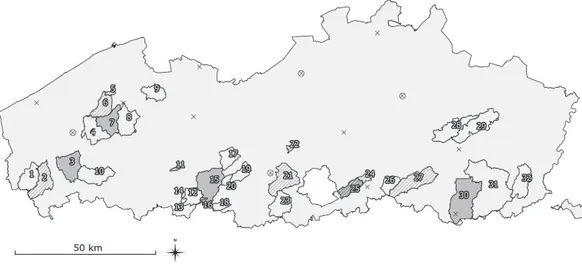
Figure 2 shows a preselection of 32 catchments in the Scheldt and Yser basins in Flan-ders. The drainage areas range from 2 to 265 km2. The size of the catchments consid-20

(7)

HESSD

10, 103–144, 2013

Title Page

Tables Figures

◭ ◮

Back Close

Full Screen / Esc

Discussion

P

a

per

|

Dis

cussion

P

a

per

|

Discussion

P

a

per

|

Discussio

n

P

a

per

|

potential evapotranspiration forcing records were obtained from the Flemish Environ-ment Agency (VMM) monitoring network. Precipitation and potential evapotranspiration time series were available for the period 2005–2010 in, respectively 14 and 4 meteo stations (see Fig. 2). The year 2005 is used to initialise the PDM. Catchment spe-cific forcing data were obtained using inverse square distance weighing (see Eq. 4). It 5

was decided to only include the three most nearby meteo stations in the interpolation (N₌3).

z(x_i,y_i,t)=

N

X

k=1

h

(x_i−x_k)2+(y_i−y_k)2i−1

N

P

j=1

(x_i−x_j)2₊₍_y

i−yj)2

−1

z(x_k,y_k,t) (4)

Hereinz(x_i,y_i,t) is the interpolated forcingzat the point of gravity (x_i,y_i) of catchment

i at timestep t. z(x_k,y_k,t) is the forcing record measured at the k-th meteo station 10

out ofN at location (x_k,y_k) and at timestep t. Furthermore, raster data with a spatial resolution of 25 m regarding land cover and soil type were obtained from the Flemish Geographical Information Agency (FGIA).

A subgroup of six catchments (see Table 2) is further selected for the calibration experiments. In the remainder of this paper these catchments are considered to be 15

ungauged and will be referred to with the term “autochtone catchments”. The subgroup is chosen in order to obtain a certain diversity with respect to geographical location, drainage area, land cover, soil type, geomorphology and morphometry. In this way a certain bias in the conclusions of the calibration experiments should be minimised. In Fig. 2 the autochtone catchments are colored gray.

(8)

HESSD

10, 103–144, 2013

Title Page

Tables Figures

◭ ◮

Back Close

Full Screen / Esc

Discussion

P

a

per

|

Dis

cussion

P

a

per

|

Discussion

P

a

per

|

Discussio

n

P

a

per

|

5 Estimation of the spectral densities

5.1 Case of spatial gauging divergence

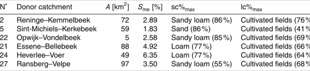
In order to estimate the density spectrum of the autochtone discharge time series in the case of spatial gauging divergence, a donor catchment approach is introduced. This implies for every autochtone catchment the identification of the catchment in the popu-5

lation of 31 remaining catchments with the most similar discharge density spectrum. In practice, this identification has to be performed indirectly because the autochtone den-sity spectrum is unknown. In this research a selection based on five catchment proper-ties is proposed to identify the best donor catchment. The difference in drainage area and the mutual distance between the points of gravity are considered to be the most 10

determining properties. The drainage area is an important indicator of the discharge magnitude and thus the spectral density magnitude. The drainage area dissimilarity between catchmentsi andj is expressed by a normalised dissimilarity index NDIA:

NDIA(i,j)=

|A_i−A_j|

A_max−A_min. (5)

A_i is the drainage area of catchmenti. The subscripts max and min indicate, respec-15

tively the highest and lowest drainage area value in the population of 32 catchments. The mutual distance between the points of gravity of two catchments can serve as a measure for the difference in the observed meteorologic pattern. Significant diff er-ences in the latter can be reflected in the spectral properties of the discharge time series. The normalised dissimilarity with respect to the mutual distance is calculated 20

by the NDID:

NDID(i,j)=

D_i_,_j

D_max. (6)

(9)

HESSD

10, 103–144, 2013

Title Page

Tables Figures

◭ ◮

Back Close

Full Screen / Esc

Discussion

P

a

per

|

Dis

cussion

P

a

per

|

Discussion

P

a

per

|

Discussio

n

P

a

per

|

the spectral density of a discharge time series is the land topography. For instance, steeper catchments are generally characterised by a higher surface runoff. Therefore, the high frequency parts of the discharge density spectrum (large k) wil be higher than will be the case in horizontal catchments. In order to let this property interfere in the selection of the donor catchments the following normalised dissimilarity index is 5

introduced:

NDI_R(i,j)= |Sme,i−Sme,j|

S_me,max−S_me,min. (7)

S_me,_i is the mean local slope of catchment i. The local slope is calculated at the grid cell scale. The subscripts max and min indicate, respectively the highest and lowest mean local slope in the population of 32 catchments. Soil composition and land cover 10

are also incorporated in the selection framework. Both properties have an important influence on the infiltration rate and thus the runoff in a catchment. Therefore, soil composition and land cover can possibly have a proper influence on the pattern of the discharge density spectrum. The NDISand NDILare proposed to, respectively account

for dissimilarities in soil composition and land cover. 15

NDI_S(i,j)=

N_B

X

k=1

φ_k |sc%k,i−sc%k,j|

sc%k,max−sc%k,min

(8)

NDIL(i,j)=

N_L

X

k=1

χ_k |lc%k,i−lc%k,j|

lc%k,max−lc%k,min

. (9)

N_BandN_Lare the number of soil and land cover classes. The relative areas of a certain soil or landcover classkare presented by sc%k and lc%k. Again, the highest and

low-20

(10)

HESSD

10, 103–144, 2013

Title Page

Tables Figures

◭ ◮

Back Close

Full Screen / Esc

Discussion

P

a

per

|

Dis

cussion

P

a

per

|

Discussion

P

a

per

|

Discussio

n

P

a

per

|

compared. In this way rare soil or land cover classes cannot have a large influence on the donor catchment selection.

To assess the total dissimilarity between two catchments a weighted sum of the aforementioned indices is calculated. In this study the following weights are used: 0.3 for the NDI_A and NDI_D, 0.2 for the NDI_S and 0.1 for the NDI_B and NDI_L. For ev-5

ery autochtone catchment the catchment with the lowest general dissimilarity is se-lected as the donor catchment. Table 3 gives an overview of the sese-lected donor catch-ments. The same order is preserved as in Table 2, so for example catchment Reninge– Kemmelbeek is the donor catchment for catchment Merkem–Martjevaart. In Fig. 2 the six donor catchments are filled in with a diagonal line pattern.

10

Subsequently, a rescaling of the donor discharge records is performed in order to improve the autochtone time series estimate. This rescaling (see Eq. 10) is based on the drainage area of the autochtone and donor catchment because of the proper linear relationship (Pearson correlation coefficientR₌0.87) between mean discharge (period 2006–2009) and the drainage area in the population of 32 Flemisch catchments. 15

ˆ

Q_aut(t)= Aaut

A_donQdon(t). (10)

ˆ

Q_aut(t) [m3s−1] is the estimated autochtone discharge time series, Q_don(t) [m3s−1] is the donor discharge time series. A_aut[km2] and A_don[km2] are the drainage areas of, respectively the autochtone and donor catchment. Based on the aforementioned rela-tionship between a time series and the corresponding spectral density spectrum, the 20

estimated density spectrum of the autochone catchment ˆS_aut(k) [m6s−2] can be calcu-lated as follows:

ˆ

S_aut(k)= A

2 aut

A2_donSdon(k). (11)

(11)

HESSD

10, 103–144, 2013

Title Page

Tables Figures

◭ ◮

Back Close

Full Screen / Esc

Discussion

P

a

per

|

Dis

cussion

P

a

per

|

Discussion

P

a

per

|

Discussio

n

P

a

per

|

of the discharge time series (period 2006–2009) in the six autochtone catchments are presented. The maximum time lag τ_max considered is 3 months. For certain catch-ments (e.g. Oostkamp–Rivierbeek and Bertem–Voer) a good match is obtained. This is however not the case for all catchments (e.g. Merkem–Martjevaart: spectral density fork₌0, Rummen–Melsterbeek: spectral densities fork >0).

5

5.2 Case of temporal gauging divergence

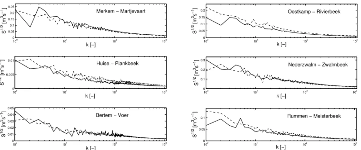
The assumption of periodicity has as consequence an invariable density spectrum. In the case of temporal gauging divergence it is thus assumed that the density spectrum of the limited non overlapping discharge time series is a good estimate of the density spectrum of the time series overlapping with the forcing records. In Fig. 5 (k=0) and 6 10

(k >0) the root squared density spectrums of the periods 2006–2007 and 2008–2009 are compared for the six catchments under consideration. A proper match is found, and this to a greater extent for the high frequency parts of the spectrums.

6 Calibration and validation

6.1 Test setup

15

In this section, different calibration experiments are carried out in order to optimise the PDM for the autochtone catchments considered in this study. The calibration period runs from 1 January 2006 through 31 December 2009. 2005 serves as a initialisation year for the RR model. The first experiment encompasses a comparison between di-rect temporal calibration and didi-rect spectral calibration. With regard to the latter, also 20

(12)

HESSD

10, 103–144, 2013

Title Page

Tables Figures

◭ ◮

Back Close

Full Screen / Esc

Discussion

P

a

per

|

Dis

cussion

P

a

per

|

Discussion

P

a

per

|

Discussio

n

P

a

per

|

domain. For both indirect calibration setups the estimates for, respectively the time se-ries and spectral density are based on discharge records at the outlet of the donor catchments. The third experiment focusses on the case of temporal gauging diver-gence. The autochtone discharge time series used in the calibration is limited and does not overlap with the forcing records. Additionally, in a fourth experiment a non overlap-5

pig donor discharge time series is used in the calibration to examine the combined effect of spatial and temporal gauging divergence on the calibration of the hydrological model. The code names and properties of all calibration setups are listed in Table 4.

Each calibration setup is applied three times for every autochtone catchment. All repeated optimisations are assessed using four indicators: the Pearson correlation co-10

efficient (R), the relative absolute bias (BIASn), the relative Root Mean Square Error (RMSEn) and the Nash-Sutcliffe coefficient (NS):

R₌

n

P

t=1

[Q_obs(t)−Q_obs][Q_sim(t)−Q_sim]

s

n

P

t=1

[Q_obs(t)−Q_obs]2

s

n

P

t=1

[Q_sim(t)−Q_sim]2

(12)

BIASn= 1

Q_obs

|1

n

X

t=1

[Q_obs(t)−Q_sim(t)]| (13)

RMSEn= 1

Q_obs

v u u t 1

n

X

t=1

[Q_obs(t)−Q_sim(t)]2 ₍₁₄₎

15

NS=1− n

P

t=1

[Q_obs(t)−Q_sim(t)]2

n

P

t=1

[Q_obs(t)−Q_obs]2

(13)

HESSD

10, 103–144, 2013

Title Page

Tables Figures

◭ ◮

Back Close

Full Screen / Esc

Discussion

P

a

per

|

Dis

cussion

P

a

per

|

Discussion

P

a

per

|

Discussio

n

P

a

per

|

Q_obs[m3s−1] andQ_sim[m3s−1] are, respectively the observed and simulated discharge values.Q_obs and Q_sim are, respectively the mean observed and simulated discharge. For every autochtone catchment and calibration setup the assessment indicators of the repetition characterised by the lowest RMSEn are retained. The absolute bias and RMSE are divided by the mean observed discharge in order to obtain four dimension-5

less indicators. In this form it is possible to average the retained indicators over the six catchments without giving more weight to the indicators of catchments characterised by a high mean discharge.

The calibration algorithm applied in this research is Particle Swarm Optimisation (PSO) (Kennedy and Eberhart, 1995). The ability of PSO to find optimal solutions for 10

hydrological modelling issues has already been demonstrated in various studies (Gill et al., 2006; Scheerlinck et al., 2009; Tolson et al., 2009; Zhang and Chiew, 2009; Mousavi and Shourian, 2010; Liu and Han, 2010; Pauwels and De Lannoy, 2011). This swarm intelligence algorithm is based on the movement of different particles through-out then-dimensional parameter space. This movement is controlled by the particle’s 15

own history of positions (and thus related values of the objective function) and that of neighbouring particles, resulting in a so-called global behaviour. In order to adjust this behaviour so that a convergence to the global optimum is found, a parametrisation of the calibration algorithm is required. The type of PSO applied in this paper is char-acterised by the parameter vectorψ₌[N_iN_kc₁c₂w δ]T (description parameters see 20

Table 5).

N_i and N_k are assigned a value of, respectively 30 and 36 (Pauwels and De Lan-noy, 2011). The values of the remaining parameters are selected out of the following discrete intervals, also applied in Pauwels and De Lannoy (2011):

1. c₁∈ {0.8, 1.0, ..., 1.8}

25

2. c₂∈ {1.0, 1.2, ..., 2.2}

(14)

HESSD

10, 103–144, 2013

Title Page

Tables Figures

◭ ◮

Back Close

Full Screen / Esc

Discussion

P

a

per

|

Dis

cussion

P

a

per

|

Discussion

P

a

per

|

Discussio

n

P

a

per

|

4. δ∈ {0.2, 0.4, 0.6}.

For every parameter combination a direct temporal calibration of the PDM is performed for the catchment Merkem–Martjevaart. The selection of the optimal parameter vector is based on the RMSE between thenobserved discharge recordsQ_obsand model sim-ulationsQ_sim. The lowest RMSE (0.637 m3s−1) is found withψ₌[30 36 1.8 2.2 0.2 0.4]T. 5

There is a problem of equifinality (Beven and Binley, 1992) as a high amount of param-eter combinations give near optimal RMSE’s. Due to practical considerations the above mentioned most optimal set is applied in all of the following calibration setups.

The model calibration is followed by a validation. The validation period runs from 1 January 2010 till 31 December 2010. For this the year 2009 is used to initialise the 10

PDM. As in the calibration the same four dimensionless indicators are used (averaged over the six autochtone catchments) to make an assessment of the calibration setups.

6.2 Results and discussion

6.2.1 Experiment 1: direct temporal vs. spectral calibration

In this first experiment direct temporal calibration is compared to direct spectral cal-15

ibration. With regard to the former the RMSE between the observed and simulated discharges is used as objective function. Spectral calibration on the other hand makes use of of a spectral objective function. For example this can be the RMSE between the spectral densities of the observed and simulated time series. However, better re-sults are achieved by an RMSE between the root squared spectral densities (Quets 20

et al., 2010; Pauwels and De Lannoy, 2011). The latter is thus applied in this research. First, the influence of the maximum lag of the correlation function τ_max on the post calibration model performance is examined. Three values forτ_max are proposed: 1, 3 and 12 months. In Fig. 7 (upper-left subplot) the averaged assessment indicators for the calibration period (2006–2009) are compared for setups T-D, F-D-1-0, F-D-3-0 and 25

(15)

HESSD

10, 103–144, 2013

Title Page

Tables Figures

◭ ◮

Back Close

Full Screen / Esc

Discussion

P

a

per

|

Dis

cussion

P

a

per

|

Discussion

P

a

per

|

Discussio

n

P

a

per

|

time domain (higherR and NS coefficient, lower BIASn and RMSEn). A clearly poorer model performance can be noted when applying a low τ_max. This is probably due to the information loss which is a consequence of the limitation of the correlation func-tion. As can be expected in the validation period (see Fig. 7, upper-right subplot) the BIASn and RMSEn are remarkably higher for all four setups compared to the calibra-5

tion period. This is however not the case for the R and NS coefficient. Furthermore, the setups relate differently with regard to model performance. For three out of four assessment indicators temporal calibration still leads to better results, however the dif-ferences with spectral calibration using aτ_maxof 3 months are very small. With respect to the relative RMSEn even better simulations are obtained after calibration in the fre-10

quency domain ifτ_maxis 1 or 3 months. Spectral calibration with the longest correlation function (τ_max₌12 months) leads to a remarkably higher BIASn and RMSEn and to a lesser extent also to a lowerR and NS coefficient. This may be due to an overfitting of the data. Because of this observation aτ_max value of 3 months is proposed for all following spectral calibration setups. A second influence on the calibration exercise ex-15

amined in this experiment is giving weights to certain parts of the density spectrum in the objective function. This is performed by the principle of exponential clustering (see Fig. 8). Three types of weights are proposed:

– Type 1: the spectral densities fork <9 retain their value. Exponential clustering and averaging over those clusters is applied fromk₌9 tok₌N. Higher weights 20

are thus assigned to the low frequency part of the density spectrum.

– Type 2: the spectral density fork₌0 is not considered in the objective function. Exponential clustering and averaging over those clusters is applied fromk₌1 to

k₌N. Higher weights are thus assigned to the low frequency part of the density spectrum with a zero weight for the first spectral density.

25

– Type 3: exponential clustering and averaging over those clusters is applied from

(16)

HESSD

10, 103–144, 2013

Title Page

Tables Figures

◭ ◮

Back Close

Full Screen / Esc

Discussion

P

a

per

|

Dis

cussion

P

a

per

|

Discussion

P

a

per

|

Discussio

n

P

a

per

|

It can be concluded from Fig. 7 (middle subplots) that giving weights to certain parts of the density spectrum generally does not lead to a better model performance in the calibration and validation period. This applies to a greater extent for weight type 3 or thus to giving more weight to the high frequency part of the density spectrum. It is also clear that not taking into account the density fork₌0 leads to a high BIASn. This 5

can be explained by the relationship between the spectral density at k₌0 and the mean of a time series. Ifτ_max₌D−1, then this first density equals the squared mean of the time series. Not taking into account the first spectral density thus results in no explicite matching of the means of the observed and simulated time series. Because of the aforementioned conclusions no types of weight are applied in the indirect spectral 10

calibrations of experiment 2, 3 and 4.

6.2.2 Experiment 2: indirect spectral calibration in case of spatial gauging divergence (setup F-IS-3-0)

This second calibration experiment focusses on the discharge prediction in an au-tochtone catchment without available discharge records at the outlet. However, dis-15

charge records are available at the outlet of a donor catchment in the same time win-dow as the forcing records monitored in the autochtone catchment (spatial gauging divergence). Two calibration strategies are undertaken: a temporal calibration on the rescaled donor discharges (see Eq. 10) (setup T-IS) and a spectral calibration on the root squared spectral densities of the rescaled donor discharges (see Eq. 11) (setup 20

F-IS-3-0). A first observation in the calibration period (see Fig. 7, lower-left subplot) is the reduced model performance after an indirect calibration compared to a direct cal-ibration. The difference is rather small forR. For the other assessment indicators the declined model performance is much clearer. Amongst others this can be explained by the rescaling of the donor discharges. Donor catchment selection and rescaling based 25

(17)

HESSD

10, 103–144, 2013

Title Page

Tables Figures

◭ ◮

Back Close

Full Screen / Esc

Discussion

P

a

per

|

Dis

cussion

P

a

per

|

Discussion

P

a

per

|

Discussio

n

P

a

per

|

Like in experiment 1,R does not change strongly in the validation period (see Fig. 7, lower-right subplot). BIASn and RMSEn on the other hand again increase significantly. Furthermore, a considerable rise of the NS coefficient can be noted for indirect tem-poral calibration in the validation period. This is not the case for indirect spectral cal-ibration. In case of spatial gauging divergence it seems to be recommended to apply 5

indirect temporal calibration. This should however be nuanced. The spatial dimensions considered in this research are rather small (magnitude kilometers). Due to this prox-imity the time lapse for a certain meteorological event to happen in the autochtone and donor catchment will be rather small (magnitude minutes-hours). If however the dis-tance between the autochtone and donor catchment is larger the time lapse increases 10

(magnitude hours–days). It is even possible that the same meteorological event will not pass over both catchments. The applicability of indirect temporal calibration should therefore be evaluated in advance based on the proximity between the autochtone and donor catchment.

6.2.3 Experiment 3: indirect spectral calibration in case of temporal gauging

15

divergence (setup F-IT-3-0)

In this experiment limited discharge records are available for the autochtone catch-ments, however, they are not contemporaneous with the forcing records. Specifically for this experiment the time window of the observed discharge time series runs from 1 January 2008 through 31 December 2009. Forcing records are available from 1 Jan-20

uary 2006 through 31 December 2007. In this way there is no overlap between the forc-ing and discharge records. The density spectrum of the observed discharge time series serves as an estimate for the density spectrum of the discharge time series concurrent with the available forcing records. The indicator values of setup F-IT-3-0 in Fig. 7 (lower-left subplot) are based on the discharge simulations over the general calibration period 25

(18)

HESSD

10, 103–144, 2013

Title Page

Tables Figures

◭ ◮

Back Close

Full Screen / Esc

Discussion

P

a

per

|

Dis

cussion

P

a

per

|

Discussion

P

a

per

|

Discussio

n

P

a

per

|

similar (R) or better indicator values (BIASn, RMSEn and NS) are obtained in case of temporal gauging divergence. This will be due to the fact that the calibration data are observed at the outlet of the autochtone catchment itself and not in a donor catchment. For the considered dataset interannual discharge variation within the same catchment is thus smaller than discharge variation between the most similar catchments within the 5

same year (in the calibration period). It should be emphasised that in this experiment the non contemporaneous discharge and forcing time series are situated very close together in time. It is not unimaginable that the assessment indicators could turn worse in case of a larger time lapse. For example many former colonies dispose of historical hydrological data because post-colonial civil warfare hindered hydrological monitoring 10

(Winsemius et al., 2006, 2009). These historical time series are often incomplete and are characterised by a larger measurement uncertainty. It is also possible that over time the meteorological conditions or the hydrological response of the catchment change, for example by an atropogene influence (Immerzeel and Droogers, 2008; Coe et al., 2011). All of this can limit the succes of indirect spectral calibration in case of temporal 15

gauging divergence. In the validation period (see Fig. 7, lower-right subplot) the fol-lowing is observed: all assessment indicators of the indirect spectral calibration (setup F-IT-3-0) are lower than those obtained with direct spectral calibration (setup F-D-3-0). Furthermore all assessment indicators of setup F-IT-3-0 exceptR are notably worse compared to those obtained in the calibration period. It can also be concluded that 20

indirect spectral calibration based on limited autochtone discharge time series (setup F-IT-3-0) results in a better model performance than indirect spectral calibration based on rescaled donor discharges (setup F-IS-3-0).

6.2.4 Experiment 4: indirect spectral calibration in case of spatio-temporal gauging divergence (setup F-IST-3-0)

25

(19)

HESSD

10, 103–144, 2013

Title Page

Tables Figures

◭ ◮

Back Close

Full Screen / Esc

Discussion

P

a

per

|

Dis

cussion

P

a

per

|

Discussion

P

a

per

|

Discussio

n

P

a

per

|

between the time windows of the donor discharges and the forcing records in the au-tochtone catchment. In this particular experimental design discharge time series are available in the donor catchment from 1 January 2008 through 31 December 2009 and forcing data from 1 January 2006 through 31 December 2007. The density spectrum of the donor discharges will serve as an estimate for the density spectrum of the au-5

tochtone discharge time series concurrent with the available forcing records. Because of the double introduced uncertainty in the calibration data it is not illogical to assume that calibration setup F-IST-3-0 would lead to a poorer model performance than setups F-IT-3-0 and F-IS-3-0. However, the assessment indicators in the calibration and valida-tion period (see Fig. 7, lower subplots) show other results. In the calibravalida-tion period the 10

assessment indicators of setup F-IST-3-0 are comparable to those of setup F-IS-3-0. Only the NS coefficient is rather lower. The validation period shows different relation-ships. The BIASn and RMSEn are remarkably better in this combined experiment than in the previous two experiments. TheR and NS coefficient are again comparable to the previous indirect spectral calibrations.

15

As illustration in Figs. 9 and 10 the scatterplots are shown resulting from the di-rect temporal calibration setup (T-D) and the four indidi-rect calibration setups (T-IS, F-IS-3-0, F-IT-3-0 and F-IST-3-0) for, respectively catchment Oostkamp–Rivierbeek and Rummen–Melsterbeek. In the former catchments very good indirect estimates of the calibration data are obtained, in the latter catchment those estimates have a lower 20

quality.

7 Conclusions

In this paper, an assessment is made of indirect calibration of the PDM for six (au-tochtone) catchments in Flanders, considered to be ungauged. As calibration algorithm PSO is applied. The described results are based on rather small catchments (mag-25

(20)

HESSD

10, 103–144, 2013

Title Page

Tables Figures

◭ ◮

Back Close

Full Screen / Esc

Discussion

P

a

per

|

Dis

cussion

P

a

per

|

Discussion

P

a

per

|

Discussio

n

P

a

per

|

(R, BIASn, RMSEn and NS). Those are averaged over the six autochtone catchments. Consequently, the discussed results are valid for an average catchment in Flanders. The first calibration experiment focuses on direct spectral calibration. For this, the root squared spectral densities of the autochtone discharge time series are incorporated in the objective function. The experiment revealed that higher values for the maximum 5

lag of the correlation function (τ_max) result in a better model performance during the calibration period. This is not necessarily the case in the validation period. This may be due to an overfitting. Furthermore giving more weight to certain parts of the density spectrum during the spectral calibration generally does not lead to better model perfor-mances. In experiments 2, 3 and 4 indirect calibration is examined in, respectively the 10

cases of spatial, temporal and spatio-temporal gauging divergence. In those cases the calibration is, respectively based on the root squared spectral densities of, respectively rescaled donor discharge records, non overlapping autochtone discharge records and non overlapping rescaled donor discharge records. Except for some specific indicator values, the model performance decreased compared to direct calibration but remained 15

at an acceptable level. With regard to indirect calibration in the case of spatial gauging divergence, slightly better results were obtained using indirect temporal calibration vs. indirect spectral calibration. Indirect temporal calibration is however impossible to exe-cute in the case of temporal and spatio-temporal gauging divergence. Therefore only indirect spectral calibration is applied in experiments 3 and 4. Generally better model 20

performances were obtained in experiment 3 compared to experiment 2. This is due to the high uncertainty associated with the estimation of a density spectrum of an au-tochtone discharge time series based on donor discharges. For certain catchments this can introduce a bias in the model results. It was expected that the model performance in experiment 4 would be worse than in experiment 2 and 3 because a double source 25

of uncertainty is introduced in the calibration data. However, the assessment indicators show that this does not have to be the case.

(21)

HESSD

10, 103–144, 2013

Title Page

Tables Figures

◭ ◮

Back Close

Full Screen / Esc

Discussion

P

a

per

|

Dis

cussion

P

a

per

|

Discussion

P

a

per

|

Discussio

n

P

a

per

|

temporal and spatio-temporal gauging divergence in ungauged catchments. Future re-search may focus on a refinement of the calibration framework (e.g. more complex objective functions, better estimation of the spectral densities, etc.). Furthermore it could be challenging but interesting to examine the link between specific catchment properties (e.g. topography, land cover, hydrological signatures, etc.) and the result-5

ing model performance after indirect calibration. For example it may be worthwile to test whether indirect spectral calibration is more suitable in catchments with a certain discharge signature.

Appendix A

Equations of the PDM

10

In the following section not further specified variables are model parameters and can be found in Table 1.

In the prepapatory first step five constants need to be calculated. The calculation of the maximum store capacity of the soil moisture storageS_max[mm] is based on the minimum (c_min[mm]) and maximum absorption capacity (c_max[mm]):

15

S_max₌b(cmin+cmax)

b₊1 . (A1)

The constantsδ₁[−],δ₂[−],ω₀[−] andω₁[−] are computed using the time constants of the first (k₁[h]) and second surface storage (k₂[h]):

δ₁₌e−k1₁ ₊_e−

1

k₂ _(A2)

δ₂₌e−k1₁_e−k1₂ _(A3)

20

ω₀=k1(e

−_k1

1 −1)−k₂(e−

1

k₂ ₋₁₎

(22)

HESSD

10, 103–144, 2013

Title Page

Tables Figures

◭ ◮

Back Close

Full Screen / Esc

Discussion

P

a

per

|

Dis

cussion

P

a

per

|

Discussion

P

a

per

|

Discussio

n

P

a

per

|

ω₁₌k2(e

−1

k₂ ₋₁₎_e−k1₁ ₋_k

1(e

−1

k₁ ₋₁₎_e−k1₂

k₂−k₁ . (A5)

The actual evapotranspiration aET [mm h−1] is calculated on the basis of the potential evapotranspiration pET [mm h−1], the store capacity in the soil moisture storageS₁[mm] 5

at the previous time step andS_max[mm].

aET(t)=pET(t) 1−

_S

max−S1(t−1)

S_max

be!

(A6)

For the calculation of the drainage Q_dr[mm h−1], S₁[mm] of the previous time step and the parametersk_g[h mm−2],S_t[mm] andb_g[−] are required:

ifS₁(t−1)≤S_t Q_dr(t)=0

ifS₁(t−1)> S_t Q_dr(t)= _k1

g(S1(t−1)−St)

b_g

.

(A7) 10

Next, the net precipitationπ[mm h−1] can be calculated as follows:

π(t)=P(t)−aET(t)−Q_dr(t). (A8)

Consequently the direct runoffQ_di[mm h−1] can be computed using the critical store capacityC∗[mm] of the previous time step,π[mm h−1] and the parameters c_min[mm],

(23)

HESSD

10, 103–144, 2013

Title Page

Tables Figures

◭ ◮

Back Close

Full Screen / Esc

Discussion

P

a

per

|

Dis

cussion

P

a

per

|

Discussion

P

a

per

|

Discussio

n

P

a

per

|

ifC∗(t−1)+π(i)< c_max

Q_di(t)=π(t)−cmax−cmin

b+1

h_c

max−C∗(t−1)

c_max−c_min

ib+1

+cmax−cmin

b+1

h_c

max−C∗(t−1)−π(t)

c_max−c_min

ib+1

ifC∗(t−1)+π(t)≥c_max

Q_di(t)=π(t)−cmax−cmin

b+1

h_c

max−C∗(t−1)

c_max−c_min

ib+1

+C∗(t−1)+π(t)−c_max.

(A9)

Once π[mm h−1] and Q_di[mm h−1] are known for the current time stepS₁[mm] can be calculated for the current time step:

ifS₁(t)≤0

S₁(t)=0

if 0< S₁(t)< S_max

S₁(t)=S₁(t−1)+π(t)−Q_di(t)

ifS₁(t)≥S_max S₁(t)=S_max.

(A10)

C∗[mm] can be calculated on the current time step on the basis ofS₁[mm] at the current 5

(24)

HESSD

10, 103–144, 2013

Title Page

Tables Figures

◭ ◮

Back Close

Full Screen / Esc

Discussion

P

a

per

|

Dis

cussion

P

a

per

|

Discussion

P

a

per

|

Discussio

n

P

a

per

|

ifC∗(t)≤0

C∗(t)=0

ifC∗(t)≥c_max

C∗(t)=c_max−(c_max−c_min)

h_S

max−S1(t)

S_max−c_min

ib+11

ifC∗(t)≥c_max C∗(t)=c_max.

(A11)

The capacity store of the subsurface storage S₃[mm] is computed usingS₃ at the previous time step,Q_drat the current time step and the parameterk_b[h].

S₃(t)=S₃(t−1)−e

−3k_bS₃2(t−1)

−1

3k_bS₃2(t−1) (

Q_dr(t)−k_bS₃3(t−1)) (A12)

Making use ofS₃[mm] andk_b[h] the base flowQ_b[mm h1] can be calculated: 5

ifQ_b(t)≤0

Q_b(t)=0

ifQ_b(t)>0

Q_b(t)=k_bS₃3(t).

(A13)

The surface runoffQ_r[mm h1] is calculated as follows:

Q_r(t)=−δ₁Q_r(t−1)−δ₂Q_r(t−2)+ω₀Q_d(t)+ω₁Q_d(t−1). (A14)

Eventually the total discharge Q_t[mm h1] can be calculated as the sum of Q_r en

Q_b:can be calculated on the current time 10

(25)

HESSD

10, 103–144, 2013

Title Page

Tables Figures

◭ ◮

Back Close

Full Screen / Esc

Discussion

P

a

per

|

Dis

cussion

P

a

per

|

Discussion

P

a

per

|

Discussio

n

P

a

per

|

Acknowledgements. The time series and spatial data analysed in this research were provided by, respectively the Flemish Environment Agency (VMM) and the Flemish Geographical Infor-mation Agency (FGIA). The authors wish to express their appreciation for this data provision. Furthermore a special acknowledgement is owed to Gabri ¨elle De Lannoy for her advice during the research.

5

References

Beven, K. and Binley, A.: The future of distributed models: model calibration and uncertainty prediction, Hydrol. Process., 6, 279–298, doi:10.1002/hyp.3360060305, 1992. 116

Brown, R. G. and Hwang, P. Y. C.: Introduction to Random Signals and Applied Kalman Filtering, John Wiley & Sons, New York, 1992. 107

10

Cabus, P.: River flow prediction through rainfall-runoff modelling with a probability-distributed model (PDM) in Flanders, Belgium, Agr. Water Manage., 95, 859–868, doi:10.1016/j.agwat.2008.02.013, 2008. 108

Coe, M. T., Latrubesse, E. M., Ferreira, M. E., and Amsler, M. L.: The effects of deforestation and climate variability on the streamflow of the Araguaia River, Brazil, Biogeochemistry, 105,

15

119–131, doi:10.1007/s10533-011-9582-2, 2011. 120

Duan, Q., Sorooshian, S., and Gupta, V.: Effective and efficient global optimization for concep-tual rainfall-runoff models, Water Resour. Res., 28, 1015–1031, doi:10.1029/91WR02985, 1992. 105

Dunne, T. and Black, R.: Partial area contributions to storm runoff in a small New-England

20

watershed, Water Resour. Res., 6, 1296, doi:10.1029/WR006i005p01296, 1970. 108 Gan, T. and Biftu, G.: Automatic calibration of conceptual rainfall-runoff models: optimization

algorithms, catchment conditions, and model structure, Water Resour. Res., 32, 3513–3524, doi:10.1029/95WR02195, 1996. 105

Gill, M. K., Kaheil, Y. H., Khalil, A., McKee, M., and Bastidas, L.: Multiobjective particle

25

swarm optimization for parameter estimation in hydrology, Water Resour. Res., 42, W07417, doi:10.1029/2005WR004528, 2006. 115

Immerzeel, W. W. and Droogers, P.: Calibration of a distributed hydrological model based on satellite evapotranspiration, J. Hydrol., 349, 411–424, doi:10.1016/j.jhydrol.2007.11.017, 2008. 120

(26)

HESSD

10, 103–144, 2013

Title Page

Tables Figures

◭ ◮

Back Close

Full Screen / Esc

Discussion

P

a

per

|

Dis

cussion

P

a

per

|

Discussion

P

a

per

|

Discussio

n

P

a

per

|

Jenson, S. and Domingue, J.: Extracting topographic structure from ditital elevation data for geographic information-system analysis, Photogramm. Eng. Rem. S., 54, 1593–1600, 1988. 108

Kennedy, J. and Eberhart, R.: Particle swarm optimization, in: Neural Networks, 1995, Proceed-ings, IEEE International Conference on, vol. 4, 1942–1948, doi:10.1109/ICNN.1995.488968,

5

1995. 105, 115

Liu, J. and Han, D.: Indices for calibration data selection of the rainfall-runoff model, Water Resour. Res., 46, W04512, doi:10.1029/2009WR008668, 2010. 115

Montanari, A. and Toth, E.: Calibration of hydrological models in the spectral do-main: An opportunity for scarcely gauged basins?, Water Resour. Res., 43, W05434,

10

doi:10.1029/2006WR005184, 2007. 106

Moore, R. J.: The PDM rainfall-runoff model, Hydrol. Earth Syst. Sci., 11, 483–499, doi:10.5194/hess-11-483-2007, 2007. 106, 135

Mousavi, S. J. and Shourian, M.: Adaptive sequentially space-filling metamodeling applied in optimal water quantity allocation at basin scale, Water Resour. Res., 46, W03520,

15

doi:10.1029/2008WR007076, 2010. 115

Papoulis, A.: Probability, Random Variables and Stochastic Processes, McGraw Hill, New York, 1965. 107

Pauwels, V. R. N. and De Lannoy, G. J. M.: Multivariate calibration of a water and energy balance model in the spectral domain, Water Resour. Res., 47, W07523,

20

doi:10.1029/2010WR010292, 2011. 106, 115, 116

Quets, J. J., De Lannoy, G. J. M., and Pauwels, V. R. N.: Comparison of spectral and time do-main calibration methods for precipitation-discharge processes, Hydrol. Process., 24, 1048– 1062, doi:10.1002/hyp.7546, 2010. 106, 116

Reed, P., Minsker, B., and Goldberg, D.: Designing a competent simple genetic algorithm for

25

search and optimization, Water Resour. Res., 36, 3757–3761, doi:10.1029/2000WR900231, 2000. 105

Scheerlinck, K., Pauwels, V. R. N., Vernieuwe, H., and De Baets, B.: Calibration of a water and energy balance model: Recursive parameter estimation versus particle swarm optimization, Water Resour. Res., 45, W10422, doi:10.1029/2009WR008051, 2009. 105, 115

30

(27)

HESSD

10, 103–144, 2013

Title Page

Tables Figures

◭ ◮

Back Close

Full Screen / Esc

Discussion

P

a

per

|

Dis

cussion

P

a

per

|

Discussion

P

a

per

|

Discussio

n

P

a

per

|

Sivapalan, M., Takeuchi, K., Franks, S., Gupta, V., Karambiri, H., Lakshmi, V., Liang, X., McDonnell, J., Mendiondo, E., O’Connell, P., Oki, T., Pomeroy, J., Schertzer, D., Uhlen-brook, S., and Zehe, E.: IAHS decade on Predictions in Ungauged Basins (PUB), 2003– 2012: shaping an exciting future for the hydrological sciences, Hydrolog. Sci. J., 48, 857–880, doi:10.1623/hysj.48.6.857.51421, 2003. 105

5

Thyer, M., Kuczera, G., and Bates, B.: Probabilistic optimization for conceptual rainfall-runoff

models: A comparison of the shuffled complex evolution and simulated annealing algorithms, Water Resour. Res., 35, 767–773, doi:10.1029/1998WR900058, 1999. 105

Tolson, B. A., Asadzadeh, M., Maier, H. R., and Zecchin, A.: Hybrid discrete dynamically dimen-sioned search (HD-DDS) algorithm for water distribution system design optimization, Water

10

Resour. Res., 45, W12416, doi:10.1029/2008WR007673, 2009. 115

Whittle, P.: Estimation and information in stationary time series, Ark. Mat., 2, 423–434, doi:10.1007/BF02590998, 1953. 106

Winsemius, H. C., Savenije, H. H. G., Gerrits, A. M. J., Zapreeva, E. A., and Klees, R.: Compar-ison of two model approaches in the Zambezi river basin with regard to model reliability and

15

identifiability, Hydrol. Earth Syst. Sci., 10, 339–352, doi:10.5194/hess-10-339-2006, 2006. 120

Winsemius, H. C., Schaefli, B., Montanari, A., and Savenije, H. H. G.: On the calibration of hy-drological models in ungauged basins: A framework for integrating hard and soft hyhy-drological information, Water Resour. Res., 45, W12422, doi:10.1029/2009WR007706, 2009. 106, 120

20

(28)

HESSD

10, 103–144, 2013

Title Page

Tables Figures

◭ ◮

Back Close

Full Screen / Esc

Discussion

P

a

per

|

Dis

cussion

P

a

per

|

Discussion

P

a

per

|

Discussio

n

P

a

per

|

Table 1.Overview of the PDM parameters with indication of the lower and upper boundaries

for catchments in Flanders.

Parameter Units Lower boundery Upper boundary

c_max [mm] 160 5000

c_min [mm] 0 300

b [–] 0.1 2

b_e [–] 1 2

k₁ [h] 0.9 40

k₂ [h] 0.1 15

k_b [h] 0 5000

k_g [h mm−2] 700 25 000

S_t [mm] 0 150

b_g [–] 1 1

tdly [h] 0 10

(29)

HESSD

10, 103–144, 2013

Title Page

Tables Figures

◭ ◮

Back Close

Full Screen / Esc

Discussion

P

a

per

|

Dis

cussion

P

a

per

|

Discussion

P

a

per

|

Discussio

n

P

a

per

|

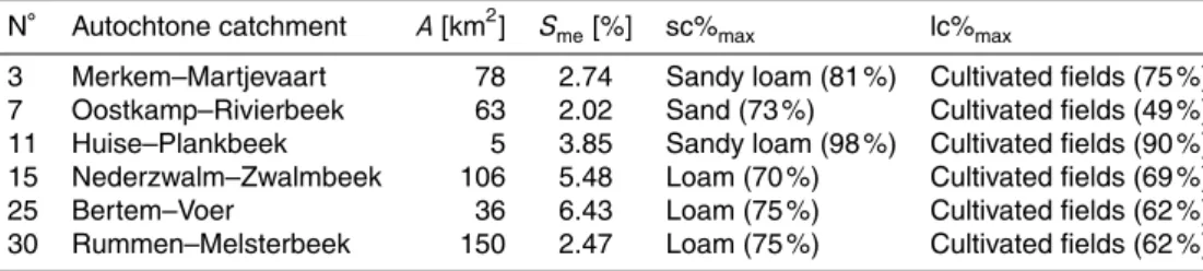
Table 2.Overview of the selected autochtone catchments and corresponding properties.Ais

the drainage area of the catchment.S_meis the local slope (mean slope of a grid cell) averaged over all grid cells within the catchment. sc%_maxand lc%_maxare, respectively the soil class and landcover class with the heighest relative area within the catchment.

N◦ Autochtone catchment A[km2] S_me[%] sc%_max lc%_max

(30)

HESSD

10, 103–144, 2013

Title Page

Tables Figures

◭ ◮

Back Close

Full Screen / Esc

Discussion

P

a

per

|

Dis

cussion

P

a

per

|

Discussion

P

a

per

|

Discussio

n

P

a

per

|

Table 3. Overview of the selected donor catchments and corresponding properties. A the

drainage area of the catchment.S_me is the local slope (mean slope of a grid cell) averaged over all grid cells within the catchment. sc%_maxand lc%_maxare, respectively the soil class and landcover class with the heighest relative area within the catchment.

N◦ Donor catchment A[km2] S_me[%] sc%_max lc%_max