Rainfall nowcasting by at site stochastic model P.R.A.I.S.E.

(1)

HESSD

4, 151–177, 2007

A new stochastic model to nowcast

rainfall at site

B. Sirangelo et al.

Title Page

Abstract Introduction

Conclusions References

Tables Figures

◭ ◮

Back Close

Full Screen / Esc

Printer-friendly Version

Interactive Discussion Hydrol. Earth Syst. Sci. Discuss., 4, 151–177, 2007

www.hydrol-earth-syst-sci-discuss.net/4/151/2007/ © Author(s) 2007. This work is licensed

under a Creative Commons License.

Hydrology and Earth System Sciences Discussions

Papers published inHydrology and Earth System Sciences Discussionsare under open-access review for the journalHydrology and Earth System Sciences

Rainfall nowcasting by at site stochastic

model P.R.A.I.S.E.

B. Sirangelo, P. Versace, and D. L. De Luca

Dipartimento di Difesa del Suolo, Universit `a della Calabria – Rende (IT)

Received: 8 January 2007 – Accepted: 19 January 2007 – Published: 29 January 2007

(2)

HESSD

4, 151–177, 2007

B. Sirangelo et al.

Title Page

Tables Figures

◭ ◮

Back Close

Full Screen / Esc

Interactive Discussion

EGU

Abstract

The paper introduces a stochastic model to forecast rainfall heights at site: the P.R.A.I.S.E. model (Prediction of Rainfall Amount Inside Storm Events). PRAISE is based on the assumption that the rainfall heightH_i₊₁ accumulated on an interval ∆t between the instantsi_∆t and (i+1)∆t is correlated with a variableZ_i(ν), representing

5

antecedent precipitation. The mathematical background is given by a joined probability densityf_H

i₊1Z( ν) i

h_i₊₁, z_i(ν) in which the variables have a mixed nature, that is a finite probability in correspondence to the null value and infinitesimal probabilities in corre-spondence to the positive values. As study area, the Calabria region, in Southern Italy, was selected, to test performances of the PRAISE model.

10

1 Introduction

Rainfall is the main input for all hydrological models such as, for example, rainfall-runoff models and for forecasting landslide induced by precipitation. In the last few years catastrophic rainfall events have occurred in the Mediterranean area, leading to floods, flash floods and shallow landslides (debris and mud flows). Consequently there

15

is the need for the implementation of forecasting systems able to predict meteorological conditions leading to disastrous occurrences. Nowadays, for achieving this goal, me-teorological and stochastic models are used. The former (Chuang et al., 2000; Palmer et al., 2000; Untch et al., 2006 ) can be viewed as valid qualitative-quantitative rainfall forecasting tools at 24, 48 and 72 h (of course, at these forecasting horizons an

abso-20

lute precision is not required, but rather an order of magnitude) when these phenomena occur on a considerable spatial scale. Nevertheless, they cannot yet be regarded as providers of quantitative rainfall forecasts in the short term (6–12 h) to be used directly for forecasting systems, since the quantitative forecasting of precipitation, on the time and space scales of the hydrological phenomena, has not yet achieved the degree of

25

(3)

HESSD

4, 151–177, 2007

B. Sirangelo et al.

Title Page

Tables Figures

◭ ◮

Back Close

Full Screen / Esc

Interactive Discussion precision necessary to avoid either the non-forecasting of exceptional small-scale

sit-uations or the issuing of unwarranted alarms. Consequently, in order to perform short term real-time rainfall forecasts for small basins (i.e. with size ranging 100–1000 km2), temporal stochastic models appear more competitive. Stochastic processes are widely used in hydrological variables forecasting and, as regards at-site models, precipitation

5

is considered as a time series with temporal coordinates at discrete points on a time axis. This set of temporal points can be known “a priori” (AutoRegressive Stochastic Models, Box and Jenkins, 1976; Salas et al., 1980; Bras and Rodriguez-Iturbe, 1984; Brockwell and Davis, 1987; Hipel and McLeod, 1994, Toth et al., 2000) or defined in a random way (Point Processes, Bartlett, 1963; Lewis, 1964; Kavvas and Delleur,

10

1981; Smith and Karr, 1983; Rodriguez-Iturbe et al., 1984; Rodriguez-Iturbe, 1986; Rodriguez-Iturbe et al., 1987; Cowpertwait, 1991; Onof and Wheater, 1994; Katz and Parlange, 1995, Cowpertwait et al., 1996; Sirangelo and Iiritano, 1997; Calenda and Napolitano, 1999; Montanari and Brath, 1999; Cowpertwait, 2004).

In the present work, a special kind of AutoRegressive model, named PRAISE

(Pre-15

diction of Rainfall Amount Inside Storm Events), is described. It can be considered as a simple and useful tool for at site nowcasting precipitation, especially for applications in rainfall-runoffmodels, regarding small basins, and forecasting landslides, induced by rainfall, models. The paper is structured in three sections, excluding the introduction: in Sect. 2 the theoretical bases of the stochastic model are illustrated; while in Sect. 3

20

model calibration is shown; finally, Sect. 4 concerns the application of the model to the raingauge network of the Calabria region, in Southern Italy, with particular regard to the Cosenza raingauge.

2 The PRAISE model

In the PRAISE model, the rainfall depthsh_n, cumulated over intervals ] (n−1)∆t, n_∆t],

25

(4)

HESSD

4, 151–177, 2007

B. Sirangelo et al.

Title Page

Tables Figures

◭ ◮

Back Close

Full Screen / Esc

EGU

random variables of mixed type, with finite probability on zero value and infinitesimal probability on positive values. In the following the instanti_∆t₌t₀is assumed as current time, so that the observed rainfall depths are with subscripts less or equal toi and the probabilistic prediction will be referred to the rainfall depths with subscripts greater than i.

5

The main feature of the approach suggested in the PRAISE model is the iden-tification of a random variable Z_i(ν), a suitable function of the ν random variables H_i, H_i₋₁, ..., H_i−ν₊₁, such that its stochastic dependence with the random variableH_i₊₁ describes the whole correlative structure of the process{H_n;n∈I}. Two steps are re-quired to identifyZ_i(ν):

10

a) the individuation of the process “memory” extensionν;

b) the optimal choice of the function depending on the random variables H_i, H_i₋₁, ..., H_i−ν₊₁definingZ_i(ν).

After this, the PRAISE model provides the identification of the joint probability density f_H

i+1Z (ν) i

h_i₊₁, z_i(ν)and its utilisation for the real time forecasting of rainfall depths during

15

a storm event.

2.1 Extension of the “memory”

In the PRAISE model, the linear stochastic dependence between the random variable H_i₊₁ and the generic antecedent random variables H_i−j, j₌0,1,2, ..., is considered negligible when the correspondent sample coefficient of partial autocorrelation results

20

less than a fixed value close to zero. The results given by this approach are similar to the more rigorous and less simple general method, in which the absence of a linear stochastic dependence should be tested verifying that the sample coefficient of partial autocorrelation, between such random variables, exhibits a value inside a confidence interval, which does not permit the rejection of the null value hypothesis for the

corre-25

spondent theoretical quantity.

In order to determine the extension of the “memory” for the process {H_n;n∈I},

(5)

HESSD

4, 151–177, 2007

B. Sirangelo et al.

Title Page Abstract Introduction Conclusions References Tables Figures ◭ ◮ ◭ ◮ Back Close

Full Screen / Esc

Interactive Discussion the absence of significant partial autocorrelation must be checked for increasing

val-ues of ν. For each value of ν must be verified the negligibility of all the sample co-efficients of partial autocorrelation characterised by a couple of primary subscripts H_i₊₁, H_i_−ν; H_i₊₁, H_i_−ν−₁; ...and by secondary subscriptsH_i, H_i−₁, ... , H_i−v₊₁. In other words, partial autocorrelation must be evaluated in the following way:

5

ρ_H

i+1Hi−ν+1−m•Hi... Hi−ν+1 = ˜ λ(ν+2)

1 (ν+2)

r ˜

λ(_{1 1}ν+2)λ˜(₍ν_ν+2)

+2) (ν+2)

m₌1,2, ... (1)

where ˜λ(_{1 (}ν+_ν2)

+2), ˜λ (ν+2) 1 1 e ˜λ

(ν+2)

(ν₊2) (ν₊2)are the cofactors of the Laurent edged matrix:

h

Λ(ν+2)i=

       

1 ρ₁ ρ₂ ... ρ_ν ρ_ν₊_m ρ₁ 1 ρ₁ ... ρ_ν−₁ρ_ν₊_m−₁ ρ₂ ρ₁ 1 ... ρ_ν−₂ρ_ν₊_m−₂ ... ... ... ... ... ... ρ_ν ρ_ν−₁ ρ_ν−₂ ... 1 ρ₁ ρ_ν₊_m ρ_ν₊_m−₁ρ_ν₊_m−₂... ρ₁ 1

        (2)

in which the autocorrelationρ_H

i+1Hi−k+1, depending only on lag k for the hypothesis of weakly stationary stochastic process, are indicated asρ_k.

10

Pratically, evaluation of ρ_H

i+1Hi−ν+1−m•Hi... Hi−ν+1 must be performed using the sample coefficients of partial autocorrelation r_H

i+1Hi−ν+1−m•Hi...Hi−ν+1, m=1,2, ..., obtained by an observed sampleh₁, h₂, ... , h_N of rainfall depths cumulated over time intervals of du-ration∆t, after estimation ofρ_kby sample autocorrelation coefficientsr_k.

Finally, to estimate the extension of the “memory”, a simple way can be obtained

15

introducing the sample maximum absolute scattering:

χ_r(ν)= max

1≤m<∞

rHi+1Hi−ν+1−m•Hi... Hi−ν+1

m=1,2, ... (3)

(6)

HESSD

4, 151–177, 2007

B. Sirangelo et al.

Title Page

Tables Figures

◭ ◮

Back Close

Full Screen / Esc

EGU

2.2 Structure of the random variableZ_i(ν)

The criterion adopted in the PRAISE model to define a functional dependence between the random variableZ_i(ν) and the random variablesH_i, H_i₋₁, ..., H_i−ν₊₁is the maximi-sation of the coefficient of linear correlation ρ_H

i+1Z (ν) i

between the same Z_i(ν) and the random variableH_i₊₁. This choice allows, once identified the joint probability density

5

f_H i+1Z

(ν) i

h_i₊₁, z_i(ν), the best prediction of rainfall depths H_i₊₁ during a storm event. If

a functional relationshipZ_i(ν) ₌ f₀₁ H_i, H_i−₁, ... , H_i_−ν₊₁

satisfies the criterion here adopted, then all the functions:

f_ab H_i, H_i₋₁, ... , H_i_−ν₊₁₌a₊b f₀₁ H_i, H_i−₁, ... , H_i−ν₊₁ (4)

withaandbgeneric constants, satisfy the same criterion. In other words, the criterion

10

of maximisation of the coefficient of linear correlation betweenZ_i(ν)andH_i₊₁identifies a “class of functions”, defined by Eq. (4), with all the members equivalent for the purposes of the suggested model.

As regards the analytical form of the relationship linkingZ_i(ν)toH_i, H_i−₁, ... , H_i−ν₊₁, the more suitable choice is, clearly, the linear function:

15

Z_i(ν) ₌β₊ ν−1

X

j₌0

α_j′H_i−j (5)

In this condition, in fact, the coe_fficients of the linear relationship that maximises ρ_H

i+1Z (ν) i

are simply the coefficients of the linear partial regression among H_i₊₁ and H_i, H_i₋₁, ..., H_i−ν₊₁:

EH_i₊₁|H_i′, H_i′

−1, ..., H

′ i−ν+1

=µ_H₊ ν−1

X

j=0

α′_jH_i′

−j (6)

20

(7)

HESSD

4, 151–177, 2007

B. Sirangelo et al.

Title Page

Tables Figures

◭ ◮

Back Close

Full Screen / Esc

Interactive Discussion where E(.) is the expected value operator, µ_H₌E(H_n), constant value for every n

because of the hypothesis of weakly stationary stochastic process, and H_i′₌H_i − µ_H, H_i′₋₁₌H_i₋₁−µ_H, H_i′_−ν₊₁₌H_i_−ν₊₁−µ_H.

Theα_j′ coefficients are evaluated as:

α_j′ ₌−λ˜(ν+1)

1(j+2)

. ˜

λ(₁₁ν+1) (7)

5

where ˜λ(ν+1)

1(j+2)e ˜λ (ν+1)

11 are the cofactors of the Laurent matrix:

h

Λ(ν+1)i=



    

1 ρ₁ ρ₂ ... ρ_ν ρ₁ 1 ρ₁ ... ρ_ν−₁ ρ₂ ρ₁ 1 ... ρ_ν−₂ ... ... ... ... ... ρ_νρ_ν−₁ρ_ν−₂... 1



    

(8)

These coefficients can be readily evaluated utilising again an observed sample h₁, h₂, ... , h_N of rainfall depths cumulated over time intervals of duration ∆t. How-ever, it should be highlighted that, as a consequence of the non-negative character of

10

the involved random variables, the coe_fficientsα_j′ must satisfy the conditionsα_j′≥0 for j₌0,1, ... , ν−1.

Moreover, the coefficientsα′_j identify, among all the possible linear combinations of H_i, H_i₋₁, ..., H_i−ν₊₁ variables, the one which maximizes the linear correlation coe_ffi -cient withH_i₊₁.

15

Then, definition ofZ_i(ν) variable is very simple: letZ(ν)

∗i be a variable defined as:

Z(ν)

∗i =µH + ν−1

X

j=0

α′_jH_i′

(8)

HESSD

4, 151–177, 2007

B. Sirangelo et al.

Full Screen / Esc

EGU

it can be noted that it is equal to the conditional expected value E H_i₊₁|H_i′, H_i′₋₁, ..., H_i−ν′ ₊₁

; rewriting Eq. (9) utilisingH_i, H_i−₁, ..., H_i_−ν₊₁:

Z(ν) ∗i =

ν−1

X

j=0

α_j′H_i−j ₊ 

1− ν−1

X

j=0

α′_j 

µ_H

and introducing the standardised coefficients:

α_j ₌α_j′ ,_ν−₁

X

κ=0

α′_κ (10)

5

for which the conditions 0 < α_j ≤1, forj₌0,1, ... , ν−1, and ν−1

P

j=0

α_j₌1 are respected,

Z(ν)

∗i can be expressed as:

Z(ν) ∗i =

ν−1

X

k=0

α_k′ ν−1

X

j=0

α_jH_i−j₊ 

1− ν−1

X

j=0

α′_j 

µH (11)

DefiningZ_i(ν)as:

Z_i(ν) ₌ ν−1

X

j=0

α_jH_i−j (12)

10

it is simple to verify thatZ(ν) ∗i and Z

(ν)

i variables are connected by a linear transforma-tion, identifying a class of functransforma-tion, defined by Eq. (4). Consequently the correlation coefficientρ_H

i+1, Z (ν) i

is equal toρ_H i+1, Z

(ν)

∗i

Equation (12) shows that the random variable Z_i(ν) can be regarded as a weighted average of theνantecedent rainfall depths with weights expressed by the coefficients

15

α_j.

(9)

HESSD

4, 151–177, 2007

B. Sirangelo et al.

Full Screen / Esc

Interactive Discussion 2.3 Joint probability densityf_H

i+1Z( ν) i

h_i₊₁, z_i(ν)

Keeping in mind the character of random variable of mixed type forH_i₊₁and, therefore, forZ_i(ν), the joint probability densityf_H

i+1Z( ν) i

h_i₊₁, z(_iν)must be written in the form:

f_H i+1,Z

(ν) i

h_i₊₁, z_i(ν)₌p_•,•δ(hi+1)δ

z(_iν)₊p₊_,• f_H(+,•)

i+1,0(hi+1)δ

z_i(ν)₊

p_•,₊f(•,+)

0,Z_i(ν)

z_i(ν)δ(h_i₊₁)+p₊_,₊f(+,+) Hi+1,Z(

ν) i

h_i₊₁, z_i(ν) (13)

where δ(.) is Dirac’s delta function,p_•,•, p₊_,•, p_•,₊ and p₊_,₊ indicate,

re-5

spectively, PrhH_i₊₁₌0∩Z_i(ν)₌0i, PrhH_i₊₁>0∩Z_i(ν)₌0i, PrhH_i₊₁₌0∩Z_i(ν)>0i and

PrhH_i₊₁>0∩Z_i(ν)>0i, with, obviously,p_•,•₊p₊_,•₊p_•,₊₊p₊_,₊₌1, and:

f(+,+) H_i₊₁,Z(ν)

i

h_i₊₁, z_i(ν)·dh_i₊₁d z_i(ν)₌

Prhh_i₊₁≤H_i₊₁< h_i₊₁₊dh_i₊₁∩z_i(ν) ≤Z_i(ν)< z_i(ν)₊d z(_iν)

Hi+1>0∩Z

(ν)

i >0 i

(14)

f_H(+,•)

i+1,0(hi+1)·dhi+1=Pr h

h_i₊₁≤H_i₊₁< h_i₊₁₊dh_i₊₁|H_i₊₁>0∩Z_i(ν)₌0i (15)

10

f(•,+)

0,Z_i(ν)

z_i(ν)·d z(_iν)₌Prhz_i(ν)≤Z_i(ν)< z_i(ν)₊d z_i(ν)

Hi+1=0∩Z

(ν)

i >0 i

(16)

A suitable mathematical form forf(+,+) Hi+1,Z(

ν) i

h_i₊₁, z_i(ν) may be achieved considering the

standardised bivariate probability density of Moran & Downton (Kotz et al., 2000):

f_X,Y (x, y)=θexp [−θ(x+y)] I₀

2 q

θ(θ−1)xy

(10)

HESSD

4, 151–177, 2007

B. Sirangelo et al.

Title Page

Tables Figures

◭ ◮

Back Close

Full Screen / Esc

EGU

whereI₀(u) is the modified Bessel functionI of zero order (Abramowitz and Stegun, 1970).

An important peculiarity of this distribution is the capacity to reproduce any positive correlative structure betweenX andY variables; they will be independent forθ₌1 and connected in deterministic way forθ→+∞.

5

Applying a double power transformation:

x₌α_h,z(h_i₊1)βh,z hi+1>0;αh,z >0, βh,z>0 (18)

y ₌γ_h,zz(_iν)δh,z z_i(ν) >0;γ_h,z >0, δh,z >0 (19)

and rewritingθasθ_h,z, the bivariate probability density so obtained, that can be called Weibull-Bessel, is given by:

10

f(+,+) Hi+1,Z

(ν) i

h_i₊₁, z_i(ν)₌θ_h,zα_h,zβ_h,z(hi+1)βh,z−1γh,zδh,z

z_i(ν) δ_h,z−1

×

exp

−θ_h,z

α_h,z(hi+1)βh,z+γh,z

z(_iν)δh,z

×

I₀ "

2 r

θ_h,z θ_h,z−1

α_h,z(hi+1)βh,zγh,z

z(_iν)δh,z #

(20)

whereh_i₊₁>0, z(_iν)>0;α_h,z>0, β_h,z>0, γ_h,z>0, δ_h,z>0, θ_h,z ≥1. As can be simply veri-fied, the marginal probability densities of the Eq. (20) are Weibull densities with

param-15

eters α_h,z, β_h,z andγ_h,z, δ_h,z. Consequently, moments of the distribution are immedi-ate, as regards means and variances:

µ(_H+,+) i+1 =E

H_i₊₁|H_i₊₁>0∩Z_i(ν) >0= Γ 1+1

β_h,z

α1

βh,z h,z

(21)

(11)

HESSD

4, 151–177, 2007

B. Sirangelo et al.

Full Screen / Esc

σ_H2 i+1

(+,+)

=v arH_i₊₁|H_i₊₁>0∩Z_i(ν)>0= 1 α2

βh,z h,z

h

Γ 1+2

β_h,z

−Γ2 1+1

β_h,zi

(22)

µ(+,+) Z_i(ν) =E

Z_i(ν)

Hi+1>0∩Z

(ν)

i >0

= Γ 1+1

δ_h,z γ1 _δ h,z h,z (23) σ2 Z(ν)

i

(+,+)

=v arZ_i(ν)

Hi+1>0∩Z (ν)

i >0

= 1 γ2 δ_h,z h,z h

Γ 1+2

δh,z

−Γ2 1+1

δh,z

i

(24)

Moreover, it can be proved that the coe_fficient of linear correlation between the random variablesH_i₊₁andZ_i(ν), distributed according to the Eq. (20), is:

5

ρ(+,+) Hi+1,Z

(ν) i

=2F1 −1

β_h,z, −1δ_h,z; 1 ; 1−1θ_h,z−1

s

Γ(1+2

β_h,z)

Γ2₍₁₊₁

β_h,z) −1

·

Γ(1+2

δ_h,z)

Γ2₍₁₊₁

δ_h,z) −1

(25)

whereΓ(u) is the complete gamma function and2F1(a, b;c;u) is the hypergeometric

function (Abramowitz and Stegun, 1970). It must be pointed out how higher values of θ_h,z parameter give higher values ofρ(+,+)

Hi+1,Z( ν) i

.

As regards the couple of probability densities f_H(+,•)

i+1,0(hi+1) and f

(•,+) 0,Z(ν) i

z_i(ν), the

10

PRAISE model, in the form here employed, assumes again Weibull densities with pa-rameters, respectively,α_h,•, β_h,•andγ_•,z, δ_•,z:

f_H(+,•)

i+1,0(hi+1)=αh,•βh,•(hi+1)

βh,•−1_exph₋_α

h,•(hi+1)βh,•

i

h_i₊₁>0;α_h,•>0, β_h,•>0 (26)

f(•,+)

0,Z(ν)

z_i(ν)₌γ_•,zδ_•,zz_i(ν)δ•,z−1exp

−γ_•,zz(_iν)δ•,z

(12)

HESSD

4, 151–177, 2007

B. Sirangelo et al.

Full Screen / Esc

EGU

3 Parameter estimation

The parameter estimation for the bivariate probability density f_H i+1Z

(ν) i

h_i₊₁, z(_iν) can be made on the basis of a sampleh₁, h₂, ... , h_N of rainfall depths cumulated over time intervals of duration∆t. First of all, starting from the sampleh₁, h₂, ... , h_Nand using the Eq. (12), a “sample” ofZ(ν) can be calculated, namelyz(₁ν), z(₂ν), ..., z_N(ν). The

prob-5

abilitiesp_•,•,p₊_,•,p_•,₊ and p₊_,₊, could be then estimated (according to the maximum likelihood method) by the frequenciesN(•,•).N,N(+,•).N,N(•,+).N andN(+,+).N of

the eventsH_i₊₁₌0∩Z_i(ν)₌0,H_i₊₁>0∩Z_i(ν)₌0,H_i₊₁₌0∩Z_i(ν)>0 andH_i₊₁>0∩Z_i(ν) >0 evaluated on the basis of the bivariate sampleh₁, z₁(ν); h₂, z₂(ν);...;h_N, z_N(ν). According to the method of moments, the parametersα_h,•, β_h,• and γ_•,z, δ_•,z could be estimated

10

fitting means and standard deviationsm(_H+,•) i+1,s

(+,•)

Hi+1 andm

(•,+)

Z_i(ν) ,s

(•,+)

,Z_i(ν) of the bivariate sam-pleh₁, z₁(ν); h₂, z(₂ν);...;h_N, z_N(ν) restricted, respectively, by the conditions, h_j>0, z(_jν)=0

andh_j₌0, z(_jν)>0.

ˆ

β_h,•₌β_h,• : Γ 1+2 β_h,•.

Γ2 1+1 β_h,•

=1+s_H2 i+1

(+,•) ,

m(_H+,•)

i+1 2

(28)

ˆ α_h,•₌

Γ1+1.βˆ_h,•

m(_H+,•) i+1

βˆh,•

(29)

15

ˆ

δ_•,z ₌δ_•,z : _Γ 1₊2 δ_•,z.

Γ2 1₊1 δ_•,z

=1₊

s2

Z_i(ν)

(•,+), m(•,+)

Z_i(ν) 2

(30)

ˆ γ_•,z₌

Γ1+1.δˆ_•,z

m(•,+) Z(ν)

i δˆ•,z

(31)

(13)

HESSD

4, 151–177, 2007

B. Sirangelo et al.

Full Screen / Esc

Interactive Discussion Similarly, the parameters of the Weibull-Bessel density, α_h,z, β_h,z,γ_h,z, δ_h,z and θ_h,z

could be estimated fitting the marginal means and standard deviations m(_H+,+) i+1 , s

(+,+)

Hi+1 andm(+,+)

Z_i(ν) ,s

(+,+)

Z_i(ν) , and the coefficient of linear correlationr

(+,+)

Hi+1,Z( ν) i

of the bivariate

sam-pleh₁, z₁(ν); h₂, z(₂ν);...;h_N, z_N(ν) restricted by the conditionh_j>0,z_j(ν)>0:

ˆ

β_h,z ₌β_h,z : Γ 1+2

β_h,z.

Γ2 1+1 β_h,z

=1+s2_H i+1

(+,+) m(_H+,+)

i+1 2

(32)

5

ˆ

α_h,z₌h_Γ1+1.βˆ_h,z.m(_H+,+) i+1

iβˆh,z

(33)

ˆ

δ_h,z ₌δ_h,z : Γ 1+2 δ_h,z.

Γ2 1+1 δ_h,z

=1+

s2

Z_i(ν)

(+,+), m(+,+)

Z_i(ν) 2

(34)

ˆ γ_h,z₌

Γ1+1.δˆ_h,z

m(+,+) Z_i(ν)

δˆh,z

(35)

ˆ

θ_h,z ₌θ_h,z : 2F1 −

1 ˆ β_h,z

, − 1 ˆ

δ_h,z; 1 ; 1− 1 θ_h,z

!

=1+r(+,+) Hi+1,Z

(ν) i

s_H(+,+) i+1 m(_H+,+)

i₊1 s(+,+)

Z_i(ν) m(+,+)

Z_i(ν)

(36)

Equations (28)–(30)–(32)–(34)–(36) must be solved by numerical method (Press et al.,

10

1988).

4 Application

(14)

HESSD

4, 151–177, 2007

B. Sirangelo et al.

Title Page

Tables Figures

◭ ◮

Back Close

Full Screen / Esc

EGU

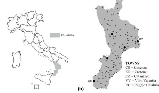
Funzionale MeteoIdrologico della Regione Calabria”. The raingauge network, located in the Calabria region, Southern Italy, is made up of 104 stations (Fig. 1). Approxi-mately, 14 million hourly rainfalls form the database, of which about 7% are rainy. In order to respect the hypothesis of stationary process, only the data measured during the “rainy season”, 1 October–31 May has been used (De Luca, 2005)

5

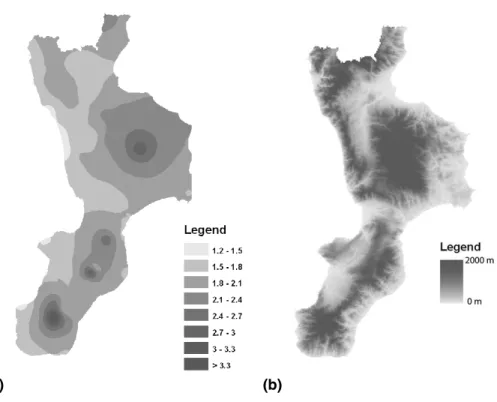
The model parameters have been estimated for every raingauge. Subsequently, each parameter was mapped on the spatial regional domain by using a spline tech-nique. The extension of the “memory”, determined by the technique described in the Sect. 2.1 fixingχ_r,cr₌0.025, has been found equal to ˆν₌8 for all the tele-metering rain-gauges. An example of parameter mapping, referred toθ_h,z is represented in Fig. 2a,

10

that shows greater values, and consequently higher values ofρ(+,+) Hi+1,Z

(ν) i

correlation,

lo-cated in the part of region characterized by greater altitude, as depicted by the com-parison with the Digital Elevation Model of the Calabria region (Fig. 2b).

Considering hourly rain measurements of the Cosenza raingauge, covering a period of about 15 years, sample autocorrelogram and memory extension are depicted in

15

Fig. 3.

The estimated coefficients ˆα_j, j₌1,2, ...,8, given by Eqs. (7–10) once calcu-lated the sample coefficients of the linear partial regression between H_i₊₁ and H_i, H_i₋₁, ..., H_i−ν₊₁, are listed in Table 1. Finally, all the parameters of the bivariate probability densityf_H

i+1Z (ν) i

h_i₊₁, z_i(ν), estimated according to the methods described

20

in section 3, are reported in Tables 2 and 3.

In Figure 4 empirical distribution functions of the variables H_i₊₁|H_i₊₁>0∩Z_i(ν)>0,

Z_i(ν)

Hi+1 > 0 ∩ Z

(ν)

i >0, Hi+1|Hi+1>0 ∩ Z

(ν)

i =0 and Z

(ν)

i

Hi+1=0 ∩ Z

(ν)

i >0, for the Cosenza raingauge, are depicted. To these empirical distributions, Weibull distribu-tion funcdistribu-tions, with parameters (αh,z, βh,z), (γh,z,δh,z), (αh,•, βh,•) and (γ•,z, δ•,z), are

25

plotted. The plots indicate that the Weibull distributions are acceptable marginals for these variables.

(15)

HESSD

4, 151–177, 2007

B. Sirangelo et al.

Title Page

Tables Figures

◭ ◮

Back Close

Full Screen / Esc

Interactive Discussion 4.1 Validation of the model

As regards rainfall forecasting, each simulation requires the knowledge of the rainfalls relative to the eight previous hours. Starting from these, simulations can be carried out for the successive hours. The temporal extension of the forecast should not exceed six hours. Beyond this limit the results become similar to the unconditional ones and, then,

5

a model update by observed precipitation is necessary.

In the applications, using the Monte Carlo technique, the simulations are carried out repeating the process 10 000 times in order to have a large synthetic sample of rainfall heights for every forecasting hour. The Monte Carlo technique is adopted because of the complexity of determining analytical probabilistic distributions for rainfall heights

10

relative to forecasting the hours successive to the first one. For these distributions, convolution operations should be required.

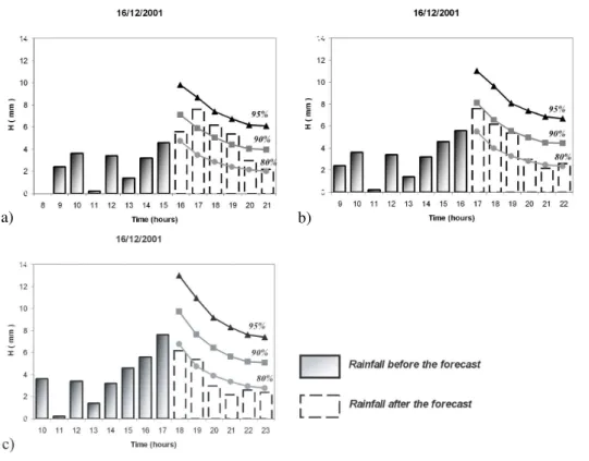
As an example, in this paper the applications relative to 19 November 1996 (Fig. 5) for the Cosenza raingauge, and 16 December 2001 (Fig. 6) for the Catanzaro rain-gauge are illustrated.

15

For every event, the real values of the precipitation have been compared with the percentiles 80%, 90% and 95% of the probabilistic distributions of every forecasting hour. Moreover, for every event the PRAISE model was applied shifting the starting point of forecasting for three successive hours.

The Figs. 5–6 show that rainfall heights of the real event fall between percentiles

20

80% and 90%. These results indicate the capability of the model to identify, for the forecast hours, statistical confidence limits containing the real rainfall heights.

5 Conclusions

This paper presents a new stochastic model named PRAISE to forecast rainfall heights at site. The mathematical background is characterized by a bivariate probability

distri-25

(16)

HESSD

4, 151–177, 2007

B. Sirangelo et al.

Title Page

Tables Figures

◭ ◮

Back Close

Full Screen / Esc

EGU

site and antecedent precipitation in the same site.

The peculiarity of PRAISE is the availability of the probabilistic distributions of rainfall heights for the forecasting hours, conditioned by the values of observed precipitation.

PRAISE was applied to all the telemetering raingauges of the Calabria region, in Southern Italy; the calibration model shows that the hourly rainfall series present a

5

constant value of memoryνequal to 8 h, for every raingauge of the Calabria network. Moreover, analysingθ_h,zparameter mapping, it must be pointed out how higher values ofρ(+,+)

Hi+1,Z (ν) i

correlation are located in the part of region characterized by greater altitude.

The examples of validation, presented here, regarding the Cosenza and Catanzaro raingauges, indicate the capability of the model to identify, for the forecasting hours,

10

statistical confidence limits containing the real rainfall heights. The PRAISE model therefore can be considered a very useful and simple tool for forecasting precipitation and consequently, using rainfall-runoffmodels or hydro-geotechnical models, floods or landslides, in planning and managing a warning system.

References

15

Abramowitz, M. and Stegun, I. A.: Handbook of mathematical functions, Dover, New York, 1970.

Bartlett, M. S.: The Spectral Analysis of Point Processes, J. R. Stat. Soc., B25, 264–296, 1963. Box, G. E. P. and Jenkins, G. M.: Time series analysis: forecasting and control, Holden-Day.

S.Francisco, 1976. 20

Bras, R. L. and Rodriguez-Iturbe, I.: Random functions and hydrology, Dover Publications, 1984.

Brockwell, P. J. and Davis, R. A .: Time Series. Theory and Methods, Springer Verlag, New York, NY, 1987.

Calenda, G. and Napolitano, F.: Parameter estimation of Neyman–Scott processes for temporal 25

point rainfall simulation, J. Hydrol., 225, 45–66, 1999.

Chuang, Hui-Ya, and Sousounis, P. J.: A technique for generating idealized initial and boundary conditions for the PSU-NCAR Model MM5, Mon. Wea. Rev., 128, 2875–2882, 2000.

(17)

HESSD

4, 151–177, 2007

B. Sirangelo et al.

Title Page

Tables Figures

◭ ◮

Back Close

Full Screen / Esc

Cowpertwait, P. S. P.: Further developments of the Neyman-Scott clustered point process for modelling rainfall, Water Resour. Res., 27, 1431–1438, 1991.

Cowpertwait, P. S. P., O’Connell, P. E., Metcalfe, A. V., and Mawdsley, J. A.: Stochastic point process modelling of rainfall. I. Single site fitting and validation, J. Hydrol., 175, 17–46, 1996. Cowpertwait, P. S. P.: Mixed rectangular pulses models of rainfall, Hydrol. Earth Syst. Sci., 8(5), 5

993–1000, 2004.

De Luca, D. L.: Metodi di previsione dei campi di pioggia. Tesi di Dottorato di Ricerca, Universit `a della Calabria, Italy, 2005.

Hipel, K. W. and McLeod, A. I.: Time series Modeling of Water Resources and Environmental Systems, Elsevier Science, 1994.

10

Katz, R. W. and Parlange, M. B.: Generalizations of chain-dependent processes : application to hourly precipitation, Water Resour. Res., 31(5), 1331–1341, 1995.

Kavvas, M. L. and Delleur, J. W.: A stochastic cluster model of daily rainfall sequences, Water Resour. Res., 17(4), 1151–1160, 1981.

Kotz, S., Balakrishanan, N., and Johnson N. L.: Continuous Multivariate Distributions – Models 15

And Applications, Wiley, New York, NY, 2000.

Lewis, P. A. W.: Stochastic Point Processes, Wiley, New York, NY, 1964.

Montanari, A. and Brath, A.: Maximum likelihood estimation for the seasonal Neyman-Scott rectangular pulses model for rainfall, Proc. of the EGS Plinius Conference, 297–309, Maratea, Italy, 1999.

20

Onof, C. and Wheater, H. S.: Improved fitting of the Bartlett-Lewis Rectangular Pulse model for hourly rainfall, Hydrol. Sci. J., 39(6), 663–680, 1994.

Palmer, T. N., Brankovic, C., Buizza, R., Chessa, P., Ferranti, L., Hoskins, B. J., and Simmons, A. J.: A review of predictability and ECMWF forecast performance, with emphasis on Europe, ECMWF Research Department Technical Memorandum n. 326, ECMWF, Shinfield Park, 25

Reading RG2-9AX, UK, 2000.

Press, W. H., Flannery, B. P., Teukolsky, S. A., and Vetterling, W. T.: Numerical Recipes in C. The art of scientific computing, Cambrige University Press, 1988.

Rodriguez-Iturbe, I., Gupta, V. K., and Waymire, E.: Scale consideration in modelling of tempo-ral rainfall, Water Resour. Res., 20(11), 1611–1619, 1984.

30

Rodriguez-Iturbe, I.: Scale of fluctuation of rainfall models, Water Resour. Res., 22(9), 15S– 37S, 1986.

(18)

HESSD

4, 151–177, 2007

B. Sirangelo et al.

Title Page

Tables Figures

◭ ◮

Back Close

Full Screen / Esc

EGU point processes, Proc. Royal Soc. London, A 410, 269–288, 1987.

Salas, J. D., Delleur, J. W., Yevjevich, V., and Lane, W. L.: Applied modelling of hydrologic time series, Water Resources Publications, Littleton, CO, 1980.

Sirangelo, B. and Iiritano, G.: Some aspects of the rainfall analysis through stochastic models, Excerpta, 11, 223–258, 1997.

5

Smith, J. A. and Karr, A. F.: A point process model of summer season rainfall occurrences, Water Resour. Res., 19(1), 95–103, 1983.

Toth, E., Brath, A., and Montanari, A.: Comparison of short-term rainfall prediction models for real-time flood forecasting, J. Hydrol., 239(1), 132–147, 2000.

Untch, A., Miller, M., Hortal, M., Buizza, R., and Janssen, P.: Towards a global meso-scale 10

model: the high-resolution system TL799L91 & TL399L62 EPS, Newsletter n. 108, ECMWF, Shinfield Park, Reading RG2-9A, UK, 2006.

(19)

HESSD

4, 151–177, 2007

B. Sirangelo et al.

Title Page

Tables Figures

◭ ◮

Back Close

Full Screen / Esc

Table 1.Cosenza raingauge: estimated values of theα_jcoefficients.

lagk 1 2 3 4 5 6 7 8

ˆ

(20)

HESSD

4, 151–177, 2007

B. Sirangelo et al.

Title Page

Tables Figures

◭ ◮

Back Close

Full Screen / Esc

EGU

Table 2.Cosenza raingauge: estimated values ofp_•,•,p₊_,•,p_•,₊andp₊_,₊.

ˆ

p_•,• pˆ₊_,• pˆ_•,₊ pˆ₊_,₊

0.76 0.01 0.14 0.09

(21)

HESSD

4, 151–177, 2007

B. Sirangelo et al.

Title Page

Tables Figures

◭ ◮

Back Close

Full Screen / Esc

Table 3. Cosenza raingauge: estimated parameters of the densities f(+,+) Hi₊1,Z

(ν)

i

h_i₊₁, z_i(ν),

f_H(+,•)

i+1,0(hi+1) andf

(•,+) 0,Z_i(ν)

z_i(ν).

1

α_h,z β_h,z 1

γ_h,z δ_h,z θ_h,z 1

α_h,• β_h,• 1

γ_•,z δ_•,z

(mm) (mm) (mm) (mm)

(22)

HESSD

4, 151–177, 2007

B. Sirangelo et al.

Title Page

Tables Figures

◭ ◮

Back Close

Full Screen / Esc

EGU

(a) (b)

Fig. 1. (a)Location of the Calabria region, in the Southern Italy;(b)Telemetering Raingauge Network.

(23)

HESSD

4, 151–177, 2007

B. Sirangelo et al.

Title Page

Tables Figures

◭ ◮

Back Close

Full Screen / Esc

(a) (b)

(24)

HESSD

4, 151–177, 2007

B. Sirangelo et al.

Title Page

Tables Figures

◭ ◮

Back Close

Full Screen / Esc

EGU

(a)

(b)

Fig. 3. (a)Sample autocorrelogram (rainy season);(b)memory extension.

(25)

HESSD

4, 151–177, 2007

B. Sirangelo et al.

Title Page

Tables Figures

◭ ◮

Back Close

Full Screen / Esc

(a) (b)

(c) (d)

Fig. 4. Cosenza raingauge: plots on Weibull probabilistic papers of empirical and Weibull distributions for the variables (a) H_i₊₁|H_i₊₁>0 ∩ Z_i(ν) > 0; (b) Z_i(ν)

Hi+1>0 ∩ Z (ν)

i >0; (c) H_i₊₁|H_i₊₁>0∩Z_i(ν)=0;(d) Z_i(ν)

Hi+1=0∩Z (ν)

(26)

HESSD

4, 151–177, 2007

B. Sirangelo et al.

Title Page

Tables Figures

◭ ◮

Back Close

Full Screen / Esc

EGU

Fig. 5.Application of PRAISE Model relative to 19 November 1996, for the Cosenza raingauge, starting from(a)11:00 LT;(b)12:00 LT;(c)13:00 LT.

(27)

HESSD

4, 151–177, 2007

B. Sirangelo et al.

Title Page

Tables Figures

◭ ◮

Back Close

Full Screen / Esc