APPLICATION OF STOCHASTIC MODELS TO DETERMINE CUSTOMERS LIFETIME VALUE FOR A BRAZILIAN SUPERMARKETS NETWORK
Annibal Parracho Sant’Anna* Rodrigo Otavio de Araujo Ribeiro Universidade Federal Fluminense (UFF) Niterói – RJ
[email protected]; [email protected] [email protected]
* Corresponding author / autor para quem as correspondências devem ser encaminhadas
Recebido em 01/2008; aceito em 09/2008 após 1 revisão
Received January 2008; accepted September 2008 after one revision
Abstract
This paper studies strategies to access customer lifetime value (CLV). Traditionally, heuristics based on recency, frequency and monetary value variables (RFM) are used to determine the best customers. Here, some forms of directly exploring these parameters to predict CLV are compared to an approach based on fitting a stochastic model. The model employed is a composition of a model for the number of transactions along the residual lifetime and a model for the value spent. New evidence is raised on the effect of aggregating transactions monthly. The data analyzed refer to two years of purchases of a group of customers of the same entrance cohort of a fidelity program cadastre of a supermarkets network in Rio de Janeiro. Using the first year to calibrate and the second year to validate the models, good fit of both models to the series of individual data and coherent CLV predictions are obtained.
Keywords: customer lifetime value; knowledge management; marketing; retail; modeling.
Resumo
Este artigo estuda estratégias para avaliar o valor do tempo de vida do cliente (CLV). Tradicionalmente, heurísticas baseadas em variáveis medindo recência, freqüência e valor monetário (RFM) são utilizadas para determinar os melhores clientes. Aqui, algumas formas de explorar diretamente estes parâmetros para predizer o CLV são comparadas com uma abordagem baseada no ajustamento de um modelo estocástico. O modelo utilizado é uma composição de um modelo para o número de transações ao longo da vida útil residual e um modelo para o valor gasto. Nova evidência é levantada sobre o efeito de agregação das transações mensalmente. Os dados analisados referem-se a dois anos da compras de um grupo de clientes da mesma coorte de ingresso no cadastro de um programa de fidelidade de uma rede de supermercados do Rio de Janeiro. Usando o primeiro ano para calibrar e o segundo ano para validar os modelos, bom ajuste dos dois modelos para as séries de dados individuais e previsões coerentes para o CLV são obtidas.
1. Introduction
In recent years, customization and globalization tendencies drive marketing strategists to simultaneously search for knowledge on clients and to center this knowledge on few essential aspects affecting their relationship to the firms. Progress in data management, on the other side, offers a huge volume of information, covering a large set of variables from which some may be chosen. The concept of customer lifetime value (CLV) is the basis of a methodology designed to extract summary information from databases on customers and their transactions with the firm. It is based on the exploration of data summarized in three simple statistics: recency, frequency and monetary value (RFM).
CLV may be defined as the present value of the total margin of contribution of each customer to a firm’s profit along all the time of such customer’s relationship with that firm from now on. CLV is measured like the discounted cash flow in Finance. There are two essential differences however. First, CLV is measured on an individual or segment level. Second, CLV measurement takes into account the chance of future random events such as the customer migrating to a competitor or, by any other reason, stop the use of the services or products of the firm at any time.
Here, a stochastic approach to predict CLV on the basis of past relationship is studied. This study is based on the empirical analysis of the adjustment of statistical models to data on a cohort of customers of a Brazilian supermarkets network. Data of two years purchases of customers receiving the network fidelity card in the month of December of 2003 are employed in the parameters estimation and models validation process. Data of the first year were used to fit the models (calibration stage). The next year data are used to verify the fit (validation stage).
The strategy investigated employs a mix of stochastic models: one of them traces the number of months along which the customer will be active and the other the average amount of expenditures in each month with purchases. The product of these two measures: the number of purchases and their per month average value, eventually completed by the information on the profit margin of contribution of the sales income, will provide the individual prediction of CLV.
This article is developed as follows. Section 2 discusses the use of Data Mining in the context of Relationship Marketing. Section 3 presents the stochastic models adopted to fit the series of time and value of the transactions to predict CLV. Section 4 presents approaches to predict frequency and recency parameters. Section 5 considers the prediction of the monetary value. In Section 6 the analysis of the data of the customers of the supermarkets chain is developed. The last section comments on the main findings and possible future developments.
2. Data Mining in the Relationship Marketing
not possible to determine the end of the relationship with certainty. It becomes then necessary adopting heuristics or probabilistic models to determine the basis of active clients.
Gupta, Lehmann & Stuart (2004) list three main factors to explain the increasing interest on CLV. First, there is an increasing pressure to develop accounting measures for marketing. Traditional measures like mark perception, sales amount or market share are not enough to precisely justify the investment made on marketing. Financial information like stocks value or aggregate profit, as well as the ratios commonly extracted from the balance sheet still do not solve this problem. CLV of present and future customers provides a new proxy to the total value of a firm.
A second factor is the importance of evaluating the profitability of each customer to drive marketing efforts. Some clients the firm will better loose. Others must be dealt with in a proper manner, in order to change relationship. Such individual diagnoses cannot be derived from consolidate metrics.
The third factor is the advance in Information Technology (IT). Now each firm can collect an enormous amount of information about customer’s transactions. Besides, the advance on data modeling allows database marketing analysts to transform the millions of transactions registers into information useful for decision making. IT made possible leveling customers relationship to a higher stage, with individually customized marketing programs.
CLV has a further advantage, of not needing any mechanism to forecast social or psychological behavior. It only employs the simple quantitative concepts of old heuristics based on recency, frequency and monetary value. Hughes (2005) shows that the answer to market actions follows much more recency than any other variable. Recency may be defined as the time of the most recent purchase. Frequency is the number of purchases in a time interval. Monetary value refers to the expected amount of money spent in each transaction or time interval.
Before the introduction of the techniques of CLV modeling, it was already common weighting these three variables to generate scores of customers’ relationship. The RFM approach includes also fitting regression models employing these and other variables to predict income to be received from each customer or probability of answer to catalog mail sales effort, for instance. Many recent studies compare such scoring models with CLV metrics. Reinartz & Kumar (2003) employed data of three cohorts in B-to-C activities and data from a high technology firm in B-to-B to analyze that. They claim that, taking the future into account, CLV models provide a better identification of more profitable customers.
Different time horizons are employed in the analyses of customers’ value. Reinartz & Kumar (2003) determine it in a finite time span: customer value in the next three years, for instance. Others, like Fader, Hardie & Lee (2005a) and Gupta & Lehmann (2003), prefer the infinite time approach.
To model the monetary value of transactions, the Gamma/Gamma model (Colombo & Jiang, 1999), employed also by Fader, Hardie & Lee (2005a), will also be investigated here. Gupta & Lehmann (2005) suggest taking into account the possibility of increasing value of the margin of contribution along time. In the present study the constancy assumption is taken. Its evaluation against the assumption of different parameters for the gamma/gamma model in distinct frequency groups was performed and did not significantly improve the predictions obtained.
& Lee (2005a) employ a model to describe recency and frequency and leave acquisition out of the model. The same is done in the present study.
Gupta & Lehmann (2003) claim that, in general, CLV is around 4.5 times the margin of contribution that the customer offers the firm in the next year. They register also a retention rate generally around 60% to 90% and a discount rate between 8% and 16% a year. The present work, by fitting models for CLV to real data, intends to provide elements for a more precise measurement of such parameters.
3. Models for CLV Measurement
Schmittlein, Morrison & Colombo (1987) proposed the first model for prediction of the frequency of future purchases that, besides modeling the purchases of an active customer as a negative binomial distribution (NBD), modeled also the termination rate. This was the Pareto/NBD model. This model describes the flow of future transactions by modeling the unobserved termination as a Pareto time model (exponential–gamma mixture) and the purchases of an active customer as an NBD counting model (Poisson-gamma mixture). The implementation of this model is limited by the difficulty of estimation of its parameters. The suitability of this approach is discussed, for instance, by Balasubramanian (1998) and by Dipak & Singh (2002). Practical implementations are in Reinartz & Kumar (2000), Schmittlein & Peterson (1994) and Fader, Hardie & Lee (2005a).
Fader, Hardie & Berger (2004) developed the BG/BB model, which is going to be tested here, as a simplification of the Pareto/NBD model. It is easier to implement because it takes time as a discrete parameter. Fader, Hardie & Lee (2005b) developed the BG/NBD model as a closer alternative to the Pareto/NBD model. This last model lacks yet a suitable expression for the value of the discounted expected number of future transactions (DET), which is, as will be seen in the following, an essential measure to the computation of CLV.
To fit a BG/BB model, from each customer only three informations are needed: the number of months, x, in which purchases were made, the last month in which purchases were registered, m, and the total number of months, n, for which the possibility of purchasing was considered. This makes this model more resistant to the influence of outliers than alternatives with continuous time parameter.
By fitting this model, at least three important measures are offered to management: the probability of each customer remaining active at each future time, the expected amount of months of activity in any future time interval and DET. This last measure, combined with the expected monthly monetary value, is directly used to predict CLV.
The BG/BB model is based on five assumptions:
B1. While active, each customer buys at any opportunity of purchase with a probability p, i. e., the indicator of a transaction, of any active customer, follows a Bernoulli distribution with parameter p.
B2. The variability of p along the customers of a same firm follows a beta distribution with parameters α and β, i. e., with density
1 1
(1 )
( | , ) , 0 1 .
( , )
p p
f p p
B
α β
α β
α β
− − −
B3. Any active customer becomes inactive at the interval between any two successive opportunities of purchase with a probability q, i. e., the lifetime of any customer follows a geometric distribution with parameter q.
B4. The variability of q along the customers follows a beta distribution with parameters γ and δ, i. e., with density
1 1
(1 )
( | , ) , 0 1.
( , )
q q
f q q
B
γ δ
γ δ
γ δ
− − −
= < <
B5. The probability of transaction, p, and the probability of termination, q, vary independently along the customers.
Combining the BG/BB features, for a customer with a past flow of transactions determined by the number x of transactions during a span of n transaction opportunities and the last transaction at the m-th opportunity, the likelihood of p and q is given by
1
0
( , | , , ) (1 ) (1 ) (1 ) (1 )
n m
x n x n x m x i m i
i
L p q x n m p p q p p q q
− −
− − + +
=
= − − +
∑
− −and that of α, β, γ and δ by
1 1
0 0
( , , , | , , ) ( , | , , ) ( | , ) ( | , ) Lα β γ δ x n m =
∫∫
L p q x n m f p α β f q γ δ dpdq1
0
( , ) ( , ) ( , ) ( 1, )
( , ) ( , ) ( , ) ( , )
n m
i
B x n x B n B x m n i B m i
B B B B
α β γ δ α β γ δ
α β γ δ α β γ δ
− −
=
+ + − + + + − + + + +
= +
∑
.4. Retention and Frequency Prediction
Wübben & Wangenhein (2006) propose a simple heuristics to forecast active customers. It consists of fixing a time threshold c, such that customers that do not buy for a time larger than c are considered as definitely inactive. The value of c may be set statistically by maximizing the number of right predictions in a long-range sample.
Another way to determine if a customer is active or not is based on the events history modeling proposed by Reinartz & Kumar (2002). The probability of remaining active is estimated by(m/n)x, m denoting recency, n, total time and x, frequency, as above.
A modified estimator based on the events history model, given by (ln(m)/ln(n))x, is also tested in this study. It results in a slower decay of the number of active customers.
Finally, by the BG/BB model, the probability of a customer with a past relationship given by
n, m and x remaining active after time n is given by
1 (1 ) (1 ) ( | , , , , )
( , | , , )
x n x n
p p q
P Active x n m p q
L p q x n m
− +
− −
=
( , ) ( , 1) ( , ) ( , )
( | , , , , , , ) ( , , , | , , )
B x n x B n
B B
P Active x n m
L x n m
α β γ δ
α β γ δ
α β γ δ α β γ δ
+ + − + +
=
Other important information given by the BG/BB approach is the expected number of future transactions for a finite time horizon. Denoting by E X( *|n x n m*, , , , , , , )α β γ δ the expected number of transactions in the next n* months by a customer with past relationship described by the x, n and m,
* * ( 1, )
( | , , , , , , , )
( , )
B x n x
E X n x n m
B
α β
α β γ δ
α β
+ + + −
=
* ( 1, 1) ( 1, 1)
( , )
( , , , | , , ).
B n B n n
B
L x n m
γ δ γ δ
γ δ
α β γ δ
− + + − − + + +
×
The computation leading to this formula may be found in Fader et alii (2004).
While most methods assume an invariant transactions flow to predict CLV, by the BG/BB model it is possible to take into account fluctuations in this flow to obtain the DET, which, multiplied by the expected monetary value of a transaction, gives the CLV. Since the probability of remaining active at the beginning of month t is (1-q)t-1, the present value of the expected number of months with transactions, at a discount rate d, is given by the sum of an
infinite geometric series with the general term
1 1 1 t q p d − − ⎛ ⎞ ⎜ + ⎟
⎝ ⎠ . Performing the summation:
1
1
1 (1 )
1
t
t
q d
p p
d d q
− ∞ = − + ⎛ ⎞ = ⎜ + ⎟ + ⎝ ⎠
∑
.Multiplying this by the probability of a customer being active at the end of the n-th month:
1 1
(1 ) (1 ) (1 ) ( | , , , , )
( ) ( , / , , )
x n x n
p p q d
DET d x n m p q
d q L p q x n m
+ − − − + +
=
+ .
A final computation, taking into account the distributions of p and q, will lead to (Fader et alii, 2004):
( 1, ) ( , 1) ( / , , , , , , )
( , ) ( , )
B x n x B n
DET d x n m
B B
α β γ δ
α β γ δ
α β γ δ
+ + + − + +
= .
A simplified approach to predict CLV was suggested by Gupta & Lehmann (2003). Assuming that the client generates a profit margin f at each purchase (or time period), a discount rate d for monetary values and a constant retention rate r, then the present value of the lifetime relationship will equal
2 3
1 ...
(1 ) fr
b b b d ⎡⎣ + + + + ⎤⎦
for (1 ) r b d = + .
This results in
1 r CLV f d r ⎛ ⎞ = ⎜⎝ + − ⎟⎠.
Or, in the case of a finite lifetime t,
1 (1 ) 1
t
r r
CLV f
d r d
⎡ ⎤
⎛ ⎞ ⎛ ⎞
= ⎜ ⎟⎢ −⎜ ⎟ ⎥
+ − ⎝ + ⎠
⎝ ⎠ ⎣ ⎦.
5. Prediction of the Value of a Transaction
The Gamma/Gamma model for the monetary value of a transaction was developed by Colombo & Jiang (1999). It originates on criticism about the hypothesis of Schmittlein & Peterson (1994), of normality of the distribution of that variable. This hypothesis of normality is contradicted by the strong asymmetry of observed distributions (Fader, Hardie & Lee, 2005a). The basic assumptions of the Gamma/Gamma model are, assuming the transactions aggregated in a monthly basis:
G1. The amount G spent by any customer during a month varies randomly.
G2. The expected value of G varies along the customers, but not through time.
G3. G is independent of the distribution of the frequency of transactions.
Formally, for a customer with transactions in x months, Z1, Z2, ... , Zxdenoting the total
spent at each of such months, the average monthly expenditure is 1 x i x i Z g x = =
∑
.G4. The Zi are independent and identically distributed gamma variables. Denoting by k and v respectively, the form and scale parameters of this common distribution, it follows from well known properties of the gamma distribution that gx has a gamma distribution
with parameters kx and vx, i. e., with density 1 ( ) ( | , , ) ( ) x vxg kx kx x x
vx g e f g k v x
kx
− − =
Γ .
G5. To model the heterogeneity along customers, it is assumed for v a gamma distribution with form parameter w and scale parameter y. Finally, assuming k constant along customers, the marginal distribution for gx has a density given by
1 ( )
( | , , , )
( ) ( ) ( )
w kx kx
x
x kx w
x
y g x kx w
f g k w y x
kx w y g x
−
+
Γ +
=
Γ Γ + .
The posterior density of v is given by
( ) 1 ( ) ( | , , , , ) ( ) x v y g x kx w kx w
x x
y g x v e
g v k w y g x
kx w
− +
+ + −
+ =
so that the expected value of G for a customer with transactions in x months and average observed expenditure gx is given by
( ) ( | , , , , )
1
x x
y g x k E G k w y m m
kx w
+ =
+ −
1
1 1 1 x
w yk kx
g
kx w w kx w
−
⎛ ⎞ ⎛ ⎞
=⎜ ⎟ +⎜ ⎟
+ − − + −
⎝ ⎠ ⎝ ⎠ .
6. Case Study
The database analyzed was formed by the registers, for 5025 customers acquired in December 2003, of their purchases during the next 24 months. Vectors of values of three variables in each year were extracted from these 5025 registers. The frequency was assessed by the number of months with transactions during the year, the recency by the month of the last transaction of the year and the monetary value by the average ticket along the year.
6.1 BG/BB Adjustment
The prediction based on fitting the BG/BB model was compared to the most frequently employed heuristic. This is based on translating for the second year the frequency of the first. The comparison was done on individual and aggregate bases.
The BG/BB prediction was based on estimates for the model parameters derived from the 1st year data. The maximum likelihood estimates are given by αˆ=1, 06, βˆ=0, 52, γˆ=31,92
and ˆδ =1922, 30.
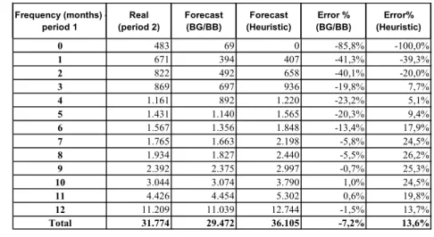
An aggregate evaluation may be done by comparing predictions for the total number of months with purchases. Table 1 presents real and predicted values for this total number of months with purchase in the second year. Such totals are presented for each subset of customers with a given number of months with purchase in the first year. This total number of months is obtained by adding the numbers of months with purchase of the customers in the subset. It is clear that, from six months on, the BG/BB model predicts better than repeating the frequency of Year 1.
Table 1 – Total cohorts numbers of months with purchase.
Frequency (months) -period 1
Real (period 2)
Forecast (BG/BB)
Forecast (Heuristic)
Error % (BG/BB)
Error% (Heuristic)
0 483 69 0 -85,8% -100,0%
1 671 394 407 -41,3% -39,3%
2 822 492 658 -40,1% -20,0%
3 869 697 936 -19,8% 7,7%
4 1.161 892 1.220 -23,2% 5,1%
5 1.431 1.140 1.565 -20,3% 9,4%
6 1.567 1.356 1.848 -13,4% 17,9%
7 1.765 1.663 2.198 -5,8% 24,5%
8 1.934 1.827 2.440 -5,5% 26,2%
9 2.392 2.375 2.997 -0,7% 25,3%
10 3.044 3.074 3.790 1,0% 24,5%
11 4.426 4.454 5.302 0,6% 19,8%
12 11.209 11.039 12.744 -1,5% 13,7%
Another form of evaluation may be derived from the comparisons of the statistical distributions of the predicted frequencies of transactions with the real distribution. Table 2 provides data for the comparison of the distribution of the individual numbers of months with purchases predicted by the BG/BB model to that of the real number observed in the second year. For six of the nine deciles, the BG/BB model generates values closer to those of Year 2 than those provided by the heuristic of translating the distribution of the previous year.
One of these deciles is the median, with a value of 6 months in Year 2 and an estimate of 6.4 on the basis of the individual predictions of the BG/BB model. The median of Year 1 was 8, offering a five times larger error. An identical result will be found if the mean is considered. The mean of the distribution of Year 2 is 6.3, and the mean of the number of months predicted by the BG/BB model is 5.9, with an underestimation of 0.4, while the mean of Year 1 is 7.2, with an overestimation more than twice larger, of 0.9.
Table 2 – Distribution of the number of months with purchase.
Deciles Year 2 BG/BB Year 1 1 0 0.4 1 2 1 1.6 3 3 3 3.1 4 4 5 4.8 6 5 6 6.4 8 6 9 8.0 9 7 10 8.8 11
8 11 10.4 12
9 12 10.4 12
A comparison may be established also on the basis of the distances between the individual predictions and the individual real values. These distances may be resumed, for instance, in terms of the mean and median quadratic and absolute errors, as in Table 3. Whatever the statistics taken, it is clear the gain derived from combining frequency and recency information in the stochastic model.
Table 3 – Distance between vectors of numbers of months with purchase.
Statistics BG/BB Heuristics
Mean square error 9.80 12.60 Median square error 2.56 4.00 Mean absolute error 2.37 2.54 Median absolute error 1.60 2.00
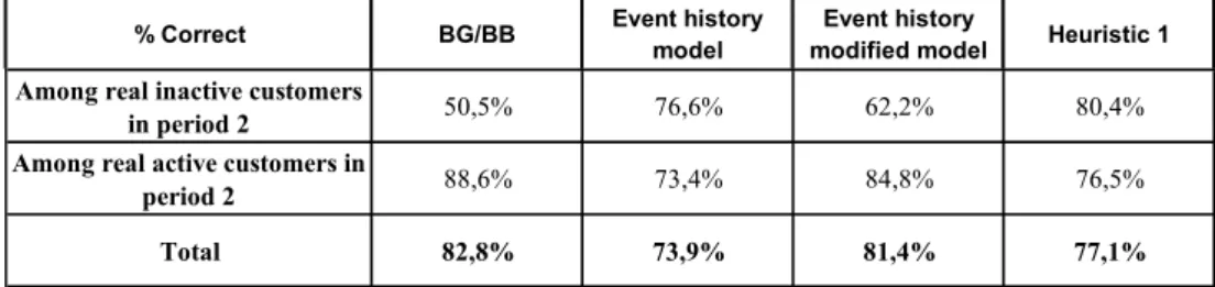
3rd column of Table 4 and by (ln(m)/ln(n))x in the 4th, is above 0.5. To apply that of Wübben & Wangenhein (2006), a customer is considered active if the last purchase was made no more than two months before (heuristic 1). In the 2nd year, a customer is considered active if it realizes at least one purchase along the year.
Table 4 – Rates of Correct Prediction of Active Condition.
% Correct BG/BB Event history
model
Event history
modified model Heuristic 1
Among real inactive customers
in period 2 50,5% 76,6% 62,2% 80,4%
Among real active customers in
period 2 88,6% 73,4% 84,8% 76,5%
Total 82,8% 73,9% 81,4% 77,1%
Table 4 summarizes the results obtained. It shows that the rate of successful prediction among the effectively inactive is the smallest for the BG/BB model, but the contrary happens among those effectively active.
In a combined strategy, of first analyzing the frequency of transactions and in a second stage predicting monetary values spent, the error of classifying as inactive a customer that remains active is worse than the opposite error of assuming that the customer is active when effectively inactive. In fact, in the second stage, customers classified as inactive will necessarily have a null monetary value, while those classified as active will have their expenditures estimated. Then, for customers wrongly classified as active, it may be expected that the model will predict low monetary values, while for customers wrongly classified as inactive no correction is possible. From this point of view, the above result, on the ability of predicting the condition of active, is once more, favorable to the BG/BB model.
6.2 Gamma/Gamma Adjustment
To evaluate the Gamma/Gamma model it is important to take into account the increase in the expenditures of the clients in the cohort due to the general increase of purchases in the network. The model is not designed to capture the effect of this increase, but to predict individual expenditure levels on the basis of the present behavior of the customers, assuming no variation in the general level of expenditure.
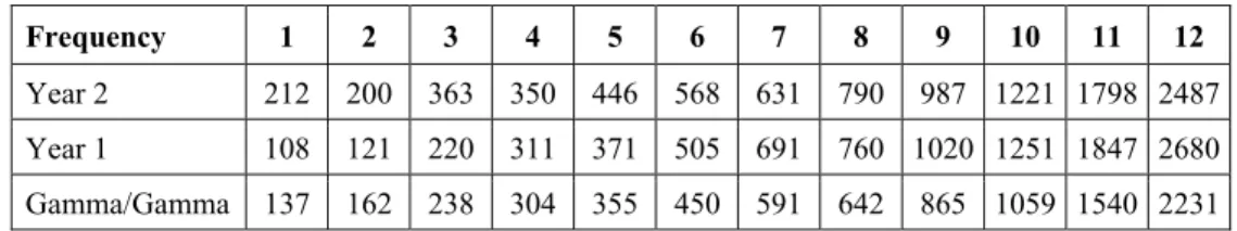
The evaluation was made initially comparing to the distribution effectively observed in the second year the distribution of individual expenditures predicted by the gamma/gamma model. The estimates obtained for the parameters were 0.39 for k 1.74 for w and 300.47 for y. Table 5 presents the average prediction by the model for each frequency class of Year 1, compared to the real observed class averages for the two years. The underestimation is present in all classes and always above 6%.
Table 5 – Statistics of the Value Distributions.
Frequency 1 2 3 4 5 6 7 8 9 10 11 12
Year 2 212 200 363 350 446 568 631 790 987 1221 1798 2487
Year 1 108 121 220 311 371 505 691 760 1020 1251 1847 2680
Gamma/Gamma 137 162 238 304 355 450 591 642 865 1059 1540 2231
6.3 Global Predictions
Global comparisons are made in terms of prediction of total outcome of Year 2. The stochastic approach predicts this total outcome of Year 2 by adding, along the whole cohort, the products of monthly outcomes predicted by the gamma/gamma model by frequencies predicted by the BG/BB model. Other predictions were obtained, following the methodology of Gupta & Lehmann (2003), improved by estimating retention rates for homogeneous groups. The customers were divided in nine groups according to their monthly frequency and according to their average income of Year 1. After calculating retention indexes for each group, the outcome estimates for Year 2 were obtained by multiplying, for each customer, the retention estimate of his or her group by the total individual outcome of Year 1.
These results are compared to the application of the simpler heuristics of assuming that the outcome of Year 2 repeats that of Year 1. All the predictions that take into account the dropout possibility are similar and much lower than the Real Income generated by the cohort each year. The point is again that the reduction in the number of active members in the cohort is, in practice, compensated by the increase in average sales from one year to the other.
Table 6 – Predictions of Year 2 Total Outcome.
0 Real Total Outcome (period 2) 5.469.270
-1 Event history model (retention rate) & Real
Total Outcome (period 1) 4.112.124 -24,8%
2 Event history modified model (retention
rate) & Real Total Outcome (period 1) 4.839.069 -11,5%
3 Heuristic 1 (retention rate) & Real Total
Outcome (period 1) 4.655.280 -14,9%
4 BG/BB & Gama-Gama 4.647.761 -15,0%
5 Real Total Outcome (period 1) 5.518.183 0,9%
Distribution Description Total Outcome Erro %
outcomes of the two years. The combination of Gamma/Gamma and BG/BB is shown to be more efficient to avoid large prediction errors. Fitting different gamma/gamma models for different frequency groups did not significantly improve that.
Table 7 – Distributions of Absolute Error.
1 2 3 4 5 6 7 8 9
0 Real Total Outcome (period 2) - - -
-1 Event history model (retention rate) & Real Total Outcome (period 1) 0 21 58 116 197 322 525 849 1.590
2 Event history modified model (retention rate) & Real Total Outcome (period 1) 2 25 63 118 204 336 520 825 1.542
3 Heuristic 1 (retention rate) & Real Total Outcome (period 1) 0 22 58 115 202 339 529 835 1.573
4 BG/BB & Gama-Gama 20 49 79 126 204 320 509 809 1.541
5 Real Total Outcome (period 1) 23 53 97 157 251 393 571 883 1.607
Distribution Description (Decile)
6.4 CLV Prediction
The quality of CLV prediction cannot be directly evaluated as long as the series of future transactions is not realized for a large enough number of years. For this reason it is important to document features of the approach taken that may be observed and numerical results obtained in a real context. An indirect form of evaluating the different strategies of CLV prediction consists in comparing properties of the distributions generated.
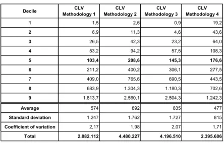
Results of the application of different methodologies are shown in Table 8. The three first approaches take as starting point the customer’s expenditure at Year 1 and combine it with the probability of remaining active according to the same three heuristics above compared. The fourth approach combines the DET generated by applying the BG/BB model with the monthly outcome predicted by the Gamma/Gamma model.
Table 8 – CLV Distributions.
Decile CLV
Methodology 1
CLV Methodology 2
CLV Methodology 3
CLV Methodology 4
1 1,5 2,6 0,9 19,2
2 6,9 11,3 4,6 43,6
3 26,5 42,3 23,2 64,0
4 53,2 94,2 57,5 108,3
5 103,4 208,6 145,3 176,6
6 211,2 400,2 306,1 277,5
7 409,0 765,6 690,5 443,5
8 683,9 1.304,3 1.180,3 702,6
9 1.813,7 2.560,1 2.504,3 1.242,3
Average 574 892 835 477
Standard deviation 1.247 1.762 1.727 815
Coefficient of variation 2,17 1,98 2,07 1,71
Table 8 registers large differences, not only in terms of the distribution of CLV but also for the total value of the cohort derived from the different distributions. The stochastic approach results in much more conservative predictions. But the smaller variation of its predictions results in a coefficient variation very close to that of the total value of the purchases of the customers (1.71 for the CLV and 1.72 for the value of the observed purchases in Year 2).
7. Final Comments
The prediction of CLV by the different methodologies studied present considerable variation. As the global predictions for the second year are similar, it is not possible to point a better approach, from an aggregate prediction point of view. Nevertheless, the analysis of the separate stages of each approach, as well as that of the dispersion of the CLV predictions, shows that the stochastic approach is able to provide more precise predictions.
The results derived from the BG/BB model are worse only when it overestimates the probability of a customer remaining active. Considering that, it is to be expected improvement in the stochastic approach from adjusting the active customers’ basis when computing expenditure parameters.
Reducing the excessive parsimony in the modeling of the expenditures to separate the customers with high monthly frequency may be also a source of improvement. Besides, taking into account other factors like purchases seasonality, variety of products bought and socioeconomic treats of the customers may improve the models.
The good fit of the BG/BB model proves the existence of a nonlinear relationship between the variables recency and frequency. Combining these variables by means of simpler prediction heuristics was also shown to generate good results. It should be taken into account, nevertheless, that the choice among these simpler alternatives asks for important subjective contributions of the analyst. The BG/BB model combines easiness of implementation with objectivity.
On the other side, the Gamma/Gamma model for the monetary values in the case presently studied provided individual estimates that combined with the BG/BB predictions resulted in sensible predictions for the CLV as well as for the outcomes generate for the following year. The predictions for the second year are smaller than the observed values, what is due to an increase in expenditures of the customers in the cohort from the first to the second year. This increase denounced a growth tendency of the whole network. This makes interesting to look for models for the monetary value that take into account the increase in sales during the period of calibration of the model.
Acknowledgements
We are grateful to the three anonymous referees for their comments.
References
(1) Balasubramanian, S.; Gupta, S.; Kamakura, W. & Wedel, M. (1998). Modeling large data sets in marketing. Statistica Neerlandica, 52(3), 303-24.
(3) Colombo, R. & Jiang, W. (1999). A stochastic RFM model. Journal of Interactive Marketing, 13, 2-12.
(4) Dipak, J. & Singh, S.S. (2002). Customer lifetime value research in Marketing: a review and future directions. Journal of Interactive Marketing, 16(2), 34-47.
(5) Fader, P.S.; Hardie, B.G.S. & Berger, P.D. (2004). Customer-base analysis with discrete-time transaction data. Available in SSRN: <http://ssrn.com/abstract=596801>.
(6) Fader, P.S.; Hardie, B.G.S. & Lee, K.L. (2005a). RFM and CLV: using iso-value curves for customer base analysis. Journal of Marketing Research, 42(4), 415-430 (7) Fader, P.S.; Hardie, B.G.S. & Lee, K.L. (2005b). Courting your customers the easy
way: an alternative to Pareto/NBD model. Marketing Science, 24(2), 275-284.
(8) Gupta, S. & Lehmann, D.R. (2003). Customers as assets. Journal of Interactive Marketing, 17, 9-24.
(9) Gupta, S. & Lehmann, D.R. (2005). Managing customers as investments: the strategic value of customers in the long run. Wharton School Publishing, New Jersey.
(10) Gupta, S.; Lehmann, D.R. & Stuart, J.A. (2004). Valuing Customers. Journal of Marketing Research, 41(1), 7-18.
(11) Hughes, A. (2005). Strategic Database Marketing. McGraw-Hill, New York.
(12) Reinartz, W.J. & Kumar, V. (2000). On the profitability of long-life customers in a noncontractual setting: an empirical investigation and implications for Marketing.
Journal of Marketing, 64(4), 17-35.
(13) Reinartz, W.J. & Kumar, V. (2002). The mismanagement of the customer loyalty.
Harvard Business Review, July, R0207F.
(14) Reinartz, W.J. & Kumar, V.(2003). The impact of customer relationship characteristics on profitable lifetime duration. Journal of Marketing, 67(1), 77-99.
(15) Reinartz, W.J.; Thomas, J. & Kumar, V. (2005). Balancing Acquisition and Retention Resources to maximize Customer Profitability. Journal of Marketing, 69(1), 63-79. (16) Schmittlein, D.C.; Morrison, D.G. & Colombo, R. (1987). Counting Your Customers:
Who They Are and What Will They Do Next? Management Science, 33, 1-24.
(17) Schmittlein, D.C. & Peterson, R.A. (1994). Customer base analysis: an industrial purchase process application. Marketing Science, 13, 41-67.