Signal Processing 85 (2005) 1059–1072
Multi-user pdf estimation based criteria for adaptive blind
separation of discrete sources
Charles Casimiro Cavalcante
a,, Joa˜o Marcos T. Romano
b aGTEL/DETI/CT/UFC, C.P. 6005, Campus do Pici, CEP: 60.455-900, Fortaleza-CE, Brazil b
DSPCom/DECOM/FEEC/UNICAMP, C.P. 6101, CEP: 13.083-852, Campinas-SP, Brazil
Received 28 April 2004; received in revised form 27 September 2004
Abstract
This paper deals with criteria for adaptive blind separation of discrete sources. The criteria are based on the estimation of the probability density function (pdf) of the recovered signal using a parametric model and the divergence of Kullback–Leibler to measure the similarities between the involved signals. Two strategies that guarantee the recovering of all sources are employed: the first one introduces a penalty when the sources are correlated and the second one constrains the filtering to an orthogonal global system response. Simulations are carried out to evaluate the performance of the criteria compared with existing blind methods in typical multi-user environments such as spatial and space-time processing.
r2005 Elsevier B.V. All rights reserved.
Keywords:Blind source separation; Discrete sources; Pdf estimation; Kullback–Leibler divergence; Constrained filtering
1. Introduction
Blind source separation (BSS) has been gaining increasing attention in the signal processing community due to its wide applicability in many fields such as digital communications, biomedical engineering and financial data analysis among others[14].
Since the milestone work by He´rault et al. in 1985[13], much effort has been done in order to
construct suitable statistical criteria that reflect some known structural properties of the sources
[19]. A common characteristic of many criteria is the use of higher order statistics (HOS), since second order statistics (SOS) are not sufficient to solve the source separation problem.
The information-theoretic approach has been introduced by Donoho in[11], who has treated the BSS problem from an entropy minimization view-point. Another well-known method to solve BSS problems is the use of contrast functions intro-duced by Comon [8], is any non-linear function which is invariant to permutation and scaling
www.elsevier.com/locate/sigpro
0165-1684/$ - see front matterr2005 Elsevier B.V. All rights reserved. doi:10.1016/j.sigpro.2004.11.023
Corresponding author. Tel.:/fax: +55 85 3288 9470.
matrices, and attains its minimum value in correspondence of the mutual independence among the output components [19]. Clearly, the methods are based in some existing requirements for BSS such as linear and time-invariant mixture, as many sensors as sources and mutually indepen-dent sources.
These works have provided important results on the issue of necessary and sufficient conditions to blindly provide source separation. Despite the development of techniques that rely directly on HOS, some single user techniques, such as constant modulus (CM) and Shalvi–Weinstein criteria, have been proposed for BSS in a single-stage and multi-single-stage context[16,20].
Multiple-input multiple-output (MIMO) sys-tems have received a lot of attention during the last decade, with several multiple access systems emerging during that time. Through BSS techni-ques, several strategies have shown promising results in the context of multiuser detection. To cite a few references, [9,17,21] reveal the potential of equalization strategies to source separation.
Papadias proposed in [19,20] a source separa-tion approach that is based on the Shalvi–Wein-stein criterion. The proposal is called multiuser kurtosis and consists of the kurtosis maximization, constrained to an orthogonal global response. It has been a great advance on the field of BSS because it has proved global convergence for an arbitrary number of users, which had not been done before.
We have previously proposed a source separa-tion criterion based on the estimasepara-tion of the probability density function (pdf) of the ideally recovered signals [5]. The criterion uses the knowledge of the pdf of transmitted signals, as in
[25], to construct a parametric model that retains the statistical properties of the source signals. Thus, the separation matrix is optimized in order to maximize the similarities between the pdf of the recovered signal and the parametric model. For this sake, we use the Kullback–Leibler divergence to measure these similarities. The criterion is then similar to the one presented in [22]; however we consider a much simpler stochastic approximation to derive an adaptive algorithm.
Our objective in this work is to propose multi-user methods based on the pdf estimation based criterion and use different strategies to ensure that all sources are recovered given some requirements (e.g., linear mixture, discrete sources). Two strategies are used for this task: (i) an auxiliary criterion that penalizes the estimated sources (outputs) that are correlated and (ii) a filtering that constrains the obtained global response to be orthogonal. Also, applications in the context of multi-user processing are presented in order to evaluate the performance of the proposals comparing them with existing blind criteria. The rest of the paper is organized as follows. The system model for memoryless and convolutive systems is described in details in Section 2. In Section 3, the pdf estimation based blind criterion is revisited in the context of SISO systems. In Section 4, the criteria for adaptive blind source separation are presented in detail, showing the different strategies for multi-user consideration. Simulation results that illustrate the performance of the proposals in some typical situations are presented in Section 5. Finally, our conclusions are stated in Section 6.
2. System model
2.1. Blind source separation: general assumptions
In the model we made the following assump-tions [26]:
(AS1) Ksources with independent and identically distributed (i.i.d.) and mutually indepen-dent zero mean discrete sequences akðnÞ;
k¼1;. . .;K:
(AS2) MIMO linear channel.
(AS3) At least as many sensors as sources.
(AS4) Noise is zero-mean, ergodic, stationary Gaussian sequence independent ofakðnÞ:
If we consider M sensors in the receiver we can represent, for instantaneous mixtures, the received signal at time instant nas
xðnÞ ¼HaðnÞ þvðnÞ, (1) whereaðnÞ ¼ ½a1ðnÞ aKðnÞ K is the vector of
M1 vector of additive noise andxðnÞis theM
1 vector of received signals.
The received signals are then processed by the MIMO equalizer given by the matrix
WðnÞ ¼ ½w1ðnÞ wKðnÞ , (2)
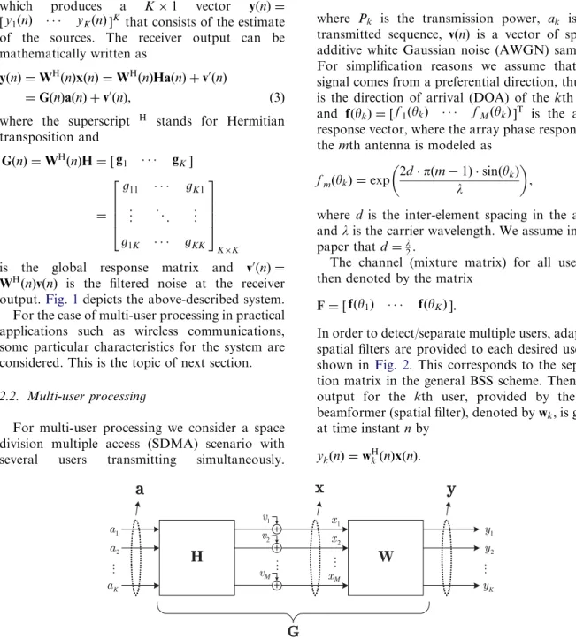
which produces a K1 vector yðnÞ ¼ ½y1ðnÞ yKðnÞ K that consists of the estimate
of the sources. The receiver output can be mathematically written as
yðnÞ ¼WHðnÞxðnÞ ¼WHðnÞHaðnÞ þv0ðnÞ
¼GðnÞaðnÞ þv0ðnÞ, ð3Þ
where the superscript H stands for Hermitian
transposition and
GðnÞ ¼WHðnÞH¼ ½g1 gK
¼
g11 gK1
. . .
. . .
. . .
g1K gKK
2 6 6 6 4
3 7 7 7 5
KK
is the global response matrix and v0ðnÞ ¼
WHðnÞvðnÞ is the filtered noise at the receiver output.Fig. 1depicts the above-described system. For the case of multi-user processing in practical applications such as wireless communications, some particular characteristics for the system are considered. This is the topic of next section.
2.2. Multi-user processing
For multi-user processing we consider a space division multiple access (SDMA) scenario with several users transmitting simultaneously.
Through the use of a linear antenna array in the receiver, we can write the discrete time model for the received signal of theK users as[7]
xðnÞ ¼X K
k¼1 ffiffiffiffiffiffi
Pk p
akðnÞ fðykÞ þvðnÞ, (4)
where Pk is the transmission power, ak is the
transmitted sequence, vðnÞ is a vector of spatial additive white Gaussian noise (AWGN) samples. For simplification reasons we assume that the signal comes from a preferential direction, thusyk
is the direction of arrival (DOA) of the kth user
and fðykÞ ¼ ½f1ðykÞ fMðykÞ T is the array
response vector, where the array phase response at themth antenna is modeled as
fmðykÞ ¼exp
2dpðm1Þ sinðykÞ l
, (5)
where d is the inter-element spacing in the array andlis the carrier wavelength. We assume in this paper that d¼l
2:
The channel (mixture matrix) for all users is then denoted by the matrix
F¼ ½fðy1Þ fðyKÞ . (6)
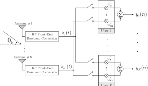
In order to detect/separate multiple users, adaptive spatial filters are provided to each desired user as shown in Fig. 2. This corresponds to the separa-tion matrix in the general BSS scheme. Then, the output for the kth user, provided by the kth beamformer (spatial filter), denoted bywk;is given
at time instant nby
ykðnÞ ¼wHkðnÞxðnÞ. (7)
Moreover, the vector of beamformers outputs is denoted byyðnÞ ¼ ½y1ðnÞ yKðnÞ T:
When intersymbol interference (ISI) is consid-ered, we have for the received signal given by convolutive mixtures the following model:
xðnÞ ¼ X K
k¼1 X Lk1
i¼0 ffiffiffiffiffiffi
Pk p
akðiÞ akðniÞ
fðyk;iÞ þvðnÞ, ð8Þ
whereakðiÞis the channel coefficient forith path of
the kth user that has a DOA yk;i and Lk is the
number of multipaths for userk:
In a matricial form, we can write the model for the mixtures[20]:
Hk¼ ffiffiffiffiffiffi
Pk p
FðykÞ ak, (9)
where
FðykÞ ¼ ½fðyk;0Þ fðyk;1Þ fðyk;Lk1Þ MLk
(10)
is a composite matrix with the steering vectors for thekth user and,
ak¼diagð½akð0Þ akð1Þ akðLk1Þ Þ (11)
is the diagonal matrix with the complex gains (amplitude and phase rotations) of the kth user channel.
In order to simplify notation, we can use some special vectors. Then, the mixture signal can be given by
XðnÞ ¼X
K
k¼1
HkAkðnÞ þVðnÞ, (12)
where
XðnÞ ¼ ½xTðnÞ xTðnNþ1Þ T
MN1,
xðnÞ ¼ ½x1ðnÞ xMðnÞ T, ð13Þ
where N is the number of coefficients in each space–time filter of the receiver;
AkðnÞ ¼½akðnÞ akðnLkNþ2Þ TðL kþN1Þ1
(14)
VðnÞ ¼ ½vTðnÞ vTðnNþ1Þ T
MN1
and vðnÞ ¼ ½v1ðnÞ vMðnÞ T. ð15Þ
The matrixHk is the channel convolution matrix
of the space–time channel for the kth user
given by[20]
where0kl is akl matrix of zeros.
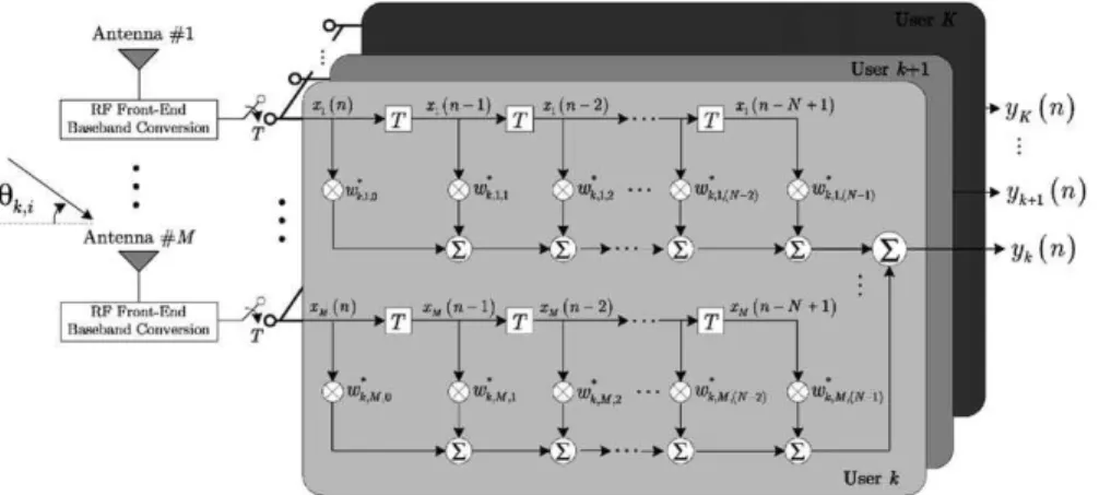
The receiver structure, which consists of a set of space–time filters is represented inFig. 3.
Then, we can write the following expressions for the estimated sources and the receiver structure: ykðnÞ ¼WH
kðnÞXðnÞ, (17)
where
Wk¼ ½wTk0 wkðN1ÞTMN1,
wT
k n_¼ ½wk;1;n
_ w
k;M;n_TM1 ð18Þ
and _n is the time index of the temporal filter associated to each antenna.
3. PDF estimation based blind criterion: SISO systems
3.1. Review
In [5] was proposed a blind criterion in the context of SISO systems (blind deconvolution). This method is revisited here.
Let wideal be an ideal zero-forcing linear
equal-izer, its output can be written as
yðnÞ ¼wHidealxðnÞ, (19)
where
xðnÞ ¼HaðnÞ þvðnÞ, (20) H is the N ðNþL1Þ convolution matrix of the single-user channel with impulse response of length L and N is the length of the impulse response of the equalizer[2].
Then, using Eq. (20) in (19), it is possible to write:
yðnÞ ¼ ðHaðnÞ þvðnÞÞHwideal ¼aHðnÞHHwidealþvHðnÞwideal ¼aHðnÞHHwideal
|fflfflfflfflffl{zfflfflfflfflffl} gideal
þvHðnÞwideal
¼aHðnÞgidealþWðnÞ
¼aðndÞ þWðnÞ, ð21Þ
Fig. 3. Space–time multi-user receiver structure.
Hk
¼
HkðnÞ 0MðN1Þ
0M1 Hkðn1Þ 0MðN2Þ
0M1 0M1 Hkðn2Þ 0MðN3Þ
. . .
..
.
0MðN1Þ HkðnNþ1Þ 2
6 6 6 6 6 6 6 6 6 4
3 7 7 7 7 7 7 7 7 7 5
MNðNþLk1Þ
where gideal is the ideal system response (a ‘‘Dirac’’-type vector), d is an arbitrary delay and WðnÞ is a random variable (r.v.) assumed Gaussian[2].
Eq. (21) states that the pdf of the signal at the output of the ideal equalizer is a mixture of Gaussians given by
pY;idealðyÞ ¼ ffiffiffiffiffiffiffiffiffiffi1
2ps2 W
q X
S
i¼1
exp jyaij 2
2s2 W
pðaiÞ,
(22)
where the ai are the possible values (scalars) of
aðndÞ; assumed to belong to the transmitted alphabetAwhich has cardinalityS.
Since the pdf of the equalized signal is known, we desire to construct a criterion that forces the adaptive filter to produce signals with the same (or as similar as possible) pdf as the ideal one. This leads to the well-known measure of similarities between strictly positive functions (such as the pdfs), theKullback–Leibler Divergence(KLD)
[12].
In order to use the KLD to provide pdf estimation, a parametric model, which is function of the filter parameters, is constructed
[2]. A natural choice is the same model of mixture of Gaussians like the one in Eq. (22) considering the estimate of the pdf of the sample yðnÞ:Then
Fðy;s2rÞ ¼ ffiffiffiffiffiffiffiffiffiffi1
2ps2 r p |fflfflffl{zfflfflffl}
A
XS
i¼1
exp jyðnÞ aij
2
2s2 r
pðaiÞ, ð23Þ
is the chosen parametric model, where s2 r is the
variance of each Gaussian in the model. In the pattern classification field this kind of parametric functions, which are used to measure similarities against other functions, are calledtarget functions
[2].
Then, applying KLD to compare the pdf of the recovered signal (equalizer output) and
(23) yields
DpðyÞjjFðy;s2
rÞ¼
Z 1
1
pðyÞln pðyÞ
Fðy;s2 rÞ dy ¼ Z 1 1
pðyÞ ln½pðyÞdy
Z 1
1
pðyÞln½Fðy;s2rÞdy. ð24Þ
This procedure aims to forcepðyÞto be ‘‘as close’’ as possible to the model given by Eq. (23) adapting the filter parameters. So, using Eq. (24) we can write the integrals as expectations over pðyÞ since such density has to be approximated to the structure given in Eq. (23).
Minimizing (24) is equivalent to minimizing only the Fðy;s2
rÞ-dependent term, and this is used
to construct our cost function, that is
JFPCðwÞ ¼ Efln½Fðy;s2rÞg
¼ E ln AX
S
i¼1
exp jyðnÞ aij 2
2s2 r
" (
pðaiÞ #)
. ð25Þ
The Fitting pdf Criterion (FPC) criterion corre-sponds to minimizing JFPCðwÞ:Furthermore, it is
known that minimizing Eq. (25) corresponds to finding the entropy of y if Fðy;s2
rÞ ¼pYðyÞ [1, p.
59].
A stochastic algorithm for filter adaptation is given by
wðnþ1Þ ¼wðnÞ mrJFPCðwÞ
rJFPCðwðnÞÞ ¼
Ps
i¼1 exp
jyðnÞaij2
2s2
r
ðyðnÞ aiÞ
s2 r
PS
i¼1exp
jyðnÞaij2
2s2
r
x;
(26) wherem is the step size.
The adaptive algorithm which uses the proposed criterion will be calledfitting pdf algorithm(FPA). Eq. (26) shows an important property of the algorithm: it takes into account the phase of the transmitted symbols.
complexity is a little higher than other blind LMS-like algorithms[10].
In the sequel we discuss some issues of the selection of the cost function and similarities with criteria previously reported in the literature.
3.2. Discussion
One important issue on the criterion design is the cost function selection. Indeed, as the KLD is a semi-distance, the order of the functions in the KLD impacts the resulting functional.
If the inverse order on KLD were taken, we would obtain
DFðy;s2
rÞkpðyÞ ¼
Z 1
1
Fðy;s2rÞln Fðy;s
2 rÞ
pðyÞ
dy
¼
Z 1
1
Fðy;s2rÞln½Fðy;s2rÞdy
Z 1
1
Fðy;s2rÞln½pðyÞdy
¼ H½Fðy;s2rÞ EFfln½pðyÞg, ð27Þ
whereH½stands for the entropy.
In this case, if the selected cost function were the one represented in Eq. (27), the resultant algo-rithm from the minimization ofDFðy;s2
rÞkpðyÞ would
be computationally more complex due to the existence of two terms dependant on the para-metric model.
Clearly, the main motivation of retaining DpðyÞjjFðy;s2
rÞ and notDFðy;s2rÞkpðyÞ concerns the
com-plexity of implementation. The analysis about possible differences on performance issues will be investigated in later works.
On the other hand, other information-theoretic approaches have been employed in the context of equalization. We briefly describe the major com-mon points of them in the sequel.
Firstly, it should be noted that the FPC can be viewed as a sort of Parzen estimation[18,23], with the center of the Gaussian kernels chosen to be the elements of the transmitted alphabet A: Using Parzen estimation for the density of the recovered data, in[18] some variations of the consideration of pdf fitting are discussed. In summary, they use the following three approaches:
Quadratic distance (QD)—the cost function is defined using the quadratic distance between the pdfs to measure the similaritiesJðwÞ ¼
Z 1
1
½pY2ðuÞ pA2ðuÞ2du, (28)
whereY2¼ fjyðnÞj2gandA2¼ fjaij2g:
Sampled pdf fitting—aims to fit the pdf only at a numberNp of representative pointsJðwÞ ¼ 1
Np XNp
i¼1
½pY2ðuiÞ Ti2, (29)
whereTi¼pA2ðuiÞ:
Matched pdf—the similarities between the de-sired pdf and the estimate are measured according toJðwÞ ¼
Z 1
1
p2Y2ðuÞpA22ðuÞdu. (30)
The resultant algorithms for the three above-mentioned criteria are somewhat similar to the FPA since the Parzen window is the Gaussian one. In [15], a clustering method is proposed also based on measure of similarities between density functions. The measure is a sort of Cauchy–Sch-wartz measure between pdfs given as
JðwÞ ¼ ln
R
pðxÞqðxÞdx
ffiffiffiffiffiffiffiffiffiffiffiffiffiffiffiffiffiffiffiffiffiffiffiffiffiffiffiffiffiffiffiffiffiffiffiffiffiffiffiffi R
p2ðxÞdxRq2ðxÞdx p
" #
, (31)
where pðxÞ and qðxÞ are pdfs of the involved signals. In this case, a Gaussian (Parzen) kernel is employed to estimate the density of recovered data, providing an adaptation procedure similar to the one in [18].
The work with major similarities is reported in
[22]. In this case, a statistical reference criterion is derived based on the use of KLD. It inserts a regeneration function to provide a recursive estimation of the data using the consideration that the noise is assumed Gaussian. Despite the very similar structure of that criterion and the FPC, the algorithms from both are quite different.
Another difference is the existence of an additional degree of freedom (parameter s2
r) in
not affect the performance of their algorithm. Particularly, the choice of such a parameter has been shown to play a key role in the cost function since the variance of the Gaussians can be used to make the estimate more robust, as discussed in details in[3].
The FPC has been generalized to the multi-user processing case as described in the next section.
4. Multi-user pdf estimation based criteria
In order to generalize the criterion to the multiple sources case, we have used the conditions for signal recovering, that are directly stated from the Shalvi–Weinstein (SW) criterion. These condi-tions can be written as[19]:
(C1) akðnÞis i.i.d. and zero meanðk¼1; . . . ;KÞ;
(C2) akðnÞ and aqðnÞ are statistically independent
forkaqand have the same pdf,
(C3) jk½ykðnÞj ¼ jkaj ðk¼1;. . .;KÞ;
(C4) EfjykðnÞj2g ¼s2a ðk¼1;. . .;KÞ;
(C5) EfykðnÞyqðnÞg ¼0; kaq;
whereakðnÞis the sequence transmitted by thekth
source,ka is the kurtosis,s2a is the variance of the
transmitted sequence, and k½ is the kurtosis operator. Conditions (C1)–(C4) are the direct interpretation of the SW theorem [24] for signal recovering and Condition (C5) guarantees achieve-ment of all the sources involved.
However, other criteria can be used to perform the signal recovering (or separation) than kurtosis maximization proposed in [24]. Since the pdf estimation approach aims, indirectly, for the equalization of all higher order statistics, FPC replaces the kurtosis maximization for interference removal.
Furthermore, the strategy for making Condition (C5) hold defines multi-user criteria as described in the sequel.
4.1. Explicit decorrelation
The first criterion uses the strategy of a penalization term that measures the cross-correla-tion of the beamformers outputs. It was initially
proposed in the context of a multi-user constant modulus algorithm (MU-CMA) in [21]. This strategy was called explicit decorrelation by[7], a nomenclature adopted in this paper.
This approach results in the following multiuser criterion [4]:
JMU-FPCðwkÞ ¼JFPCðwkÞ þg
XK
i¼1
XK
j¼1
jai
jrijj2, (32)
wheregis a regularization parameter andrijis the
correlation term between the outputs of the ith and jth beamformers. The criterion described in Eq. (32) is called multi-user fitting pdf criterion (MU-FPC).
The adaptation procedure of the MU-FPC for the kth user in a memoryless system (spatial processing) is then
wkðnþ1Þ ¼wkðnÞ mrJFPCðwkÞ
gX
K
i¼1
iak b
rikðnÞpiðnÞ, ð33Þ
wherebrikðnÞis theði;kÞelement of the matrixRyðnÞ
and piðnÞis the ith column of matrix PðnÞ;which are computed as
Ryðnþ1Þ ¼oRyðnÞ þ ð1oÞyðnÞyHðnÞ
Pðnþ1Þ ¼oPðnÞ þ ð1oÞxðnÞyHðnÞ, ð34Þ
where ois a forgetting factor. Eqs. (33) and (34) define the multi-user fitting pdf algorithm (MU-FPA).
For space–time multi-user processing it is also necessary to guarantee decorrelation of the signals in a time interval in order to remove the ISI. Thus, the criterion becomes [4]
JMU-FPCðWkÞ ¼JFPCðWkÞ
þgX
K
i¼1
XK
j¼1
jai XD2
‘¼D
2
jrijð‘Þj2, ð35Þ
where rijð‘Þ ¼EfyiðnÞyjðn‘Þgis the
cross-corre-lation between the ith and jth outputs from the space–time receivers with a time interval‘;andD
2is
The MU-FPA, for the space–time processing, is then given by[3]:
Wkðnþ1Þ ¼WkðnÞ mrJFPCðWkÞ
gX
K
i¼1
iak XD2
‘¼D
2
b
rik;‘ðnÞbpi;‘ðnÞ, ð36Þ
Ry;‘ðnþ1Þ ¼oRy;‘ðnÞ þ ð1oÞyðnÞyHðn‘Þ,
(37)
P‘ðnþ1Þ ¼oP‘ðnÞ þ ð1oÞXðnÞyHðn‘Þ, (38)
yðn‘Þ ¼ ½y1ðn‘Þ yKðn‘Þ T, (39)
‘¼ D
2;. . .;
D
2, (40)
wherebrik;‘ðnÞ is the cross-correlation between the
ith andjth users estimate with time delay‘;given by theði;jÞth element of matrix Ry;‘ðnÞ;andbpi;‘ðnÞ
is theith column of matrixP‘ðnÞ:
This criterion and its stochastic adaptive algo-rithm present good results but suffer from the strong trade-off between the number of different recovered sources (successful recovering) and steady state error w.r.t. the parameter g; due to the use of a penalization term in the multi-user criterion.
An alternative to this strategy aiming to cope with the problem of losing users (unsuccessful recovering) and a good steady state error is presented in next subsection.
4.2. Constrained criterion
Using conditions (C1)–(C5) [19] proposed a multi-user criterion based on the maximization of the kurtosis of the recovered signals named multiuser kurtosis (MUK) maximization. The recovering of all sources is ensured by a constraint that forces global response to be an orthogonal matrix.
The criterion divides the separation task into two parts: the equalization step, that maximizes the kurtosis, and the separation one, that performs the decorrelation of the outputs. For each task, we denoteWefor the equalization part, andWfor the later one. The separation is performed by means of
a Gram–Schmidt orthogonalization of matrix We [19].
However, this criterion requires a pre-whitening process on the received signals in order to assure that the variance will also be equalized.
As we have mentioned before, the use of such ‘‘decoupled’’ processing makes possible the use of equalization techniques to obtain source separa-tion, constraining the global system response to be orthogonal. The key point is that the considered equalization criterion has to respect the necessary and sufficient conditions for blind signal recover-ing.
We have noticed that the FPC can be viewed as a general case of the Shalvi–Weinstein one. This is due to the fact that equalizing the pdfs of signals corresponds to equalizing all higher-order mo-ments (cumulants) of the signals, and matching all cumulants comprises the kurtosis one, as stated by Shalvi–Weinstein and MUK criteria. Indeed, we benefit from the parametric form of pdf estimation provided by the FPC to cope with the high computational load required to match all cumu-lants between the input and output of the system. Since matching all cumulants implies matching the kurtosis, we can replace the pdf estimation procedure with the kurtosis maximization, in the MUK criterion, and the set of conditions is still valid as necessary and sufficient conditions for blind source separation. With this approach, we replace the processing with a penalization term that is performed by the MU-FPA, see Eq. 32, by a constrained procedure aiming at improving the performance. Finally, the criterion is given by
min
W JFPCðWÞ ¼ PK
j¼1
DpYðyÞkFðyj;s2
rÞ;
subject to:GHG¼cI;
8 > <
>
: (41)
Thus, the new adaptive algorithm is obtained by replacing the step of kurtosis maximization by the following computation:
Weðnþ1Þ ¼WðnÞ mwrJFPCðWðnÞÞ, (42)
where rJFPCðWðnÞÞ is given in Eq. (26) and
performing just an orthogonalization in matrix
We by means of the Gram–Schmidt procedure. The resulting algorithm is then called multiuser constrained FPA (MU-CFPA) and is summarized inTable 1.
In terms of computational complexity, the MU-CFPA is an LMS-like algorithm, although the orthogonalization procedure slightly increases the complexity of the FPA.
However, the MU-CFPA can be applied only on memoryless systems. In the case of the space–-time processing, the global response is a tensor and its orthogonalization is more complex than the matrix one.
5. Computational simulations
This section demonstrates the performance of the proposed multi-user criteria, which is com-pared to blind separation criteria found in the literature.
We have chosen three common situations in multi-user processing in order to evaluate the performance over different environments. They are described in the sequel.
5.1. Spatial multi-user processing
An SDMA system with four users is used as the evaluation scenario of the algorithms. In the receiver, we use a linear antenna array with eight elements. The DOAs for the users are the following: 1;52;29and 76:In each direction, 2000 QPSK unit power symbols are transmitted over 100 Monte Carlo trials. In this environment, we have assumed that power control is used to assure the same received power to all users, and the signal-to-noise ratio (SNR) for each sensor equals 30 dB.
In order to evaluate the performance of the proposed algorithm we use the constant modulus error (CME) defined for thekth user as follows:
CMEkðnÞ ¼ ðjykj2RÞ2. (43)
The constant R is related to the power of the transmitted constellation. In our case we will assume a normalized power, i.e., R¼1:
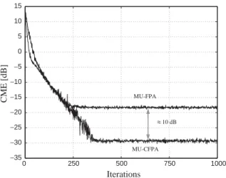
Firstly, we have investigated the gain in terms of steady state error when we use two different strategies for obtaining all sources, namely the MU-FPA and MU-CFPA. For the environment previously described, we have simulated both algorithms and observed the temporal evolution of the CME. The simulation parameters for the algorithms are: m¼103;g¼103;s2
r ¼0:1
cho-sen to achieve a CME as low as possible and initializations are performed as Wð0Þ ¼Weð0Þ ¼
Ryð0Þ ¼Pð0Þ ¼I:For the MU-FPA, the forgetting
factor used in the correlation matrices estimation is set too¼0:96:Fig. 4shows the comparison of the average CME for both algorithms.
As one can see, the MU-CFPA outperforms the MU-FPA in terms of steady state error, where the difference of performance between the two algo-rithms is about 10 dB. This is due to the dropping of the decorrelation term in Eq. (32), which eliminates the trade-off between steady state error and number of lost users [7]. In the case of MU-CFPA, this term is not taken into account, and the decorrelation procedure is done by means of the orthogonalization of the separation matrix, which improves the steady state performance. It is worth mentioning thatgwas chosen to ensure successful
Table 1 MU-CFPA 1. InitializeWð0Þ
2. forn40
3. ObtainWeðnþ1Þfrom Eqs. (42) and (26) 4. Obtainw1ðnþ1Þ ¼we1ðnþ1Þ
5. forj¼2:K
6. Compute
wjðnþ1Þ ¼wejðnþ1Þ
Xj1
l¼1
ðwHl ðnþ1Þwejðnþ1ÞÞwlðnþ1Þ
recovering of all sources without replication of a specific user (or users).
Thus, we use the CFPA instead of the MU-FPA for comparing the criterion with other known blind multi-user algorithms, namely the MU-CMA [21]. For this sake, we use the same setup and the simulation parameters for MU-CFPA described previously. The simulation para-meters are: mMU-CFPA¼4103; mMU-CMA¼
103;Wð0Þ ¼Ryð0Þ ¼Pð0Þ ¼I; o¼0:96 and g¼
103: Fig. 5shows the temporal evolution of the average CME for MU-CFPA and MU-CMA
computed over 20 independent runs (Monte Carlo trials).
Since we define convergence as the necessary number of iterations to reach the lower value of CME (or another metric), we observe that the MU-CFPA (around 300 iterations) outperforms the MU-CMA (around 2000 iterations) in terms of convergence rate and steady-state error due to the use of different decorrelation methods. The MU-CMA step size was taken as the highest one that achieves convergence. This behavior of faster convergence is due to the considered number of higher order statistics in the criteria that allow a faster estimation of the signal pdf since the MU-FPA uses much more HOS than the MU-CMA
[3,6].
5.2. Instantaneous mixtures
In this experiment, we have taken memoryless mixture matrices (instantaneous ones) for evaluat-ing the behavior of BSS algorithms on this environment.
We have considered K¼4 users transmitting QPSK unit power signals and M¼6 sensors in the receiver. The noise is inserted in each sensor with power given by SNR¼15 dB: The mixture matrix is complex valued and drawn randomly from a Gaussian zero mean and unit variance distribution for each of 100 independent trials.
Fig. 6shows the temporal evolution of the average CME for the considered algorithms. We have also included the MUK algorithm, and principal component analysis (PCA) is performed for this algorithm since pre-whitening is required. Simula-tion parameters are: mMUK¼mMU-CMA¼
4103; mMU-CFPA¼102; o¼0:98; g¼103;
s2r ¼0:2 andWð0Þ ¼Weð0Þ ¼Ryð0Þ ¼Pð0Þ ¼I:
One can easily observe that the random behavior of the mixture makes the MU-CFPA achieve the final CME at the same order of the other methods, however, it outperforms the other blind criteria w.r.t. the convergence rate. Again, this behavior is due to the use of a different number of higher order statistics by the criteria. Considering all HOS provides the observed gain [3]. The MU-CFPA was used instead of the
0 250 500 750 1000
−35 −30 −25 −20 −15 −10 −5 0 5 10 15
Iterations
CME [dB] MU-FPA
MU-CFPA 10 dB
Fig. 4. Performance evaluation of MU-FPAMU-CFPA:
0 500 1000 1500 2000 2500 3000 3500 4000
−35
−30
−25
−20
−15
−10
−5 0 5 10 15
Iterations
CM
E
[dB
]
MU-CMA
MU-CFPA
MU-FPA due to its better performance in this case of study.
5.3. Space– time multi-user processing
In this case, we considerK¼2 users transmit-ting simultaneously unit power QPSK signals. We also considerLk¼2 for the users and their relative
delays (in terms of the symbol interval T), and DOAs are shown in Table 2. Additive noise is inserted in each antenna that composes the receiver with an SNR¼30 dB: Furthermore, the pulse shape is a raised cosine with roll-off 0.35.
At the receiver, each sensor has temporal filters with N¼2 coefficients. We also consider D¼2 delayed samples for temporal decorrelation of the signals. Also, we assume that both users are recovered at a decision delay‘¼0:
A continuously trained LMS algorithm is included in this comparison as a reference for the blind algorithms. In this case, the transmitted sequences from all users are known at the receiver to update the filters making a data-aided proces-sing. It should be noted that the MU-CFPA is not used because it does not have a known space–time version. For each algorithm, we have measured the normalized residual interference (RI), which is defined as
RIkðnÞ ¼ P
ijgk;iðnÞj maxijgk;iðnÞj "
" ""
maxijgk;iðnÞj
, (44)
where gk;i is the ith component of the vector
gkðnÞ ¼WH
k H and H is a composite channel
matrix given by H¼ ½H1 H2 HK:
This figure of merit indicates the amount of residual interference that exists in each case when compared to a zero-forcing optimal solution.
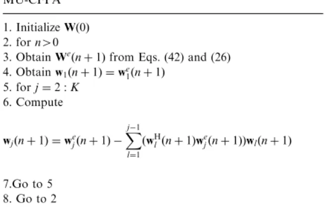
Fig. 7shows the temporal evolution of the average RI for the considered algorithms (MU-CMA and MU-FPA) under the scenario described above. The curve is an average over both users and 200 independent trials of the experiment. Simulation parameters are: mMU-FPA¼103;
mMU-CMA¼5103;mLMS¼102;o¼0:99;s2 r ¼
0:1 and Wkð0Þ ¼Ry;‘ð0Þ ¼P‘ð0Þ ¼I: It can be
seen that the MU-FPA converges much faster than the MU-CMA and slightly slower than the LMS in the initial acquisition phase. Similar performance
Table 2
Space–time system setup
User Path 1 Path 2
Delay (T) DOA (rad) Delay (T) DOA (rad)
# 1 0.1 2p
5
1.1 p
3
# 2 0.4 p
7
1.2 p
6
0 500 1000 1500 2000 2500 3000
−15 −10 5 0 5 10
Iterations
RI
[dB]
MU-CMA
MU-FPA
LMS
Fig. 7. Averaged residual interference for space–time multi-user processing.
0 1000 2000 3000 4000
−18
−16
−14
−12
−10
−8
−6
−4
−2 0
Iterations
CM
E
[dB]
MUK
MU-CMA
MU-CFPA
superiority of MU-FPA was verified over a large range of multiuser scenarios where different number of sources, relative powers, relative delays and angle displacements were considered.
6. Conclusions and perspectives
In this paper we have presented a two blind criteria based on the estimation of the probability density function of the recovered signals for adaptive blind source separation.
The criterion of interference removal is based on the maximization of the similarity between the recovered signal probability density function and a parametric model that fits the system order and transmitted signal statistical characteristics. The Kullback–Leibler divergence is then used to derive the algorithm. Two different strategies that guar-antee the recovering of the different sources involved in the process are used to construct multi-user approaches. In the first, a penalization term is inserted to force the recovered sources to be uncorrelated with each other. The latter employs a procedure that constrains the global system matrix being orthogonal so that the different fonts can be recovered.
By evaluating the proposals in typical environ-ments of multi-user communications, we have observed a better convergence rate and steady state error from our approaches compared to other existing blind criteria for the same purpose. A direct extension of this work is to derive a space–time version of the constrained algorithm using tensors to model the system and signals involved. Furthermore, an analytical analysis of the influence of the number of considered higher order statistics on the criteria is under develop-ment. Another direction is the analytical and computational comparison of different measures than KLD one to similarities between functions and different directions to KLD, as mentioned in Section 3. Afterwards, the inclusion of nonpara-metric estimation using kernels is envisaged to extend the use of the proposed methods for problems when the density of the sources is not available, such as in biomedical processing.
Acknowledgements
The authors would like to deeply thank the anonymous reviewers for their comments and suggestions that contributed a lot to the manu-script. They also thank Dr. Renato R. Lopes by his careful proofreading and comments.
References
[1] C.M. Bishop, Neural Networks for Pattern Recognition, Oxford University Press, UK, 1995.
[2] C.C. Cavalcante, Neural prediction and probability density function estimation applied to blind equalization, Master’s Thesis, Federal University of Ceara´ (UFC), Fortaleza, CE - Brazil, February 2001.
[3] C.C. Cavalcante, On blind source separation: proposals and analysis of multi-user processing strategies, Ph.D. Thesis, State University of Campinas (UNICAMP) – DECOM, Campinas, SP - Brazil, April 2004.
[4] C.C. Cavalcante, F.R.P. Cavalcanti, J.C.M. Mota, Adap-tive blind multiuser separation criterion based on log-likelihood maximisation, IEE Electron. Lett. 38 (20) (2002) 1231–1233.
[5] C.C. Cavalcante, F.R.P. Cavalcanti, J.C.M. Mota, A PDF estimation-based blind criterion for adaptive equalization, in: Proceedings of the IEEE International Symposium on Telecommunications (ITS 2002), Natal, Brazil, 2002. [6] C.C. Cavalcante, J.C.M. Mota, J.M.T. Romano,
Poly-nomial Expansion of the Probability Density Function About Gaussian Mixtures, in: Proceedings of the IEEE Workshop on Machine Learning for Signal Processing (MLSP 2004), Sa˜o Luı´s, Brazil, 2004.
[7] F.R.P. Cavalcanti, J.M.T. Romano, Blind multiuser detection in space division multiple access systems, Ann. des Te´le´commun. (7–8) (1999) 411–419.
[8] P. Comon, Independent component analysis: a new concept?, Signal Process. 36 (3) (1994) 287–314.
[9] N. Delfosse, P. Loubaton, Adaptive blind separation of independent sources: a deflation approach, Signal Process. 45 (1995) 59–83.
[10] Z. Ding, Y.G. Li, Blind Equalization and Identification, Marcel Dekker, New York, USA, 2001.
[11] D. Donoho, On Minimum Entropy Deconvolution, Academic Press, New York, 1981, pp. 565–608.
[12] S. Haykin (Ed.), Unsupervised adaptive filtering, Source Separation, vol. I, Wiley, New York, 2000.
[13] J. He´rault, C. Jutten, B. Ans, De´tection de grandeurs primitives dans un message composite par une architecture de calcul neuromime´tique en apprentissage non supervise´, in: Actes du Xe´me Colloque GRETSI, Nice, France, 1985, pp. 1017–1022.
[15] R. Jenssen, J.C. Prı´ncipe, T. Eltoft, Information cut and information forces for clustering, in: Proceedings of the IEEE Workshop on Neural Networks for Signal Proces-sing (NNSP2003), Toulose, France, 2003, pp. 459–467. [16] J.-L. Lacoume, P.-O. Amblard, P. Comon, Statistiques
d’Ordre Supe´rieur pour le Traitement du Signal, (Traite-ment du Signal), Masson, Paris, 1997.
[17] S. Lambotharan, J.A. Chambers, A.G. Constatinides, Adaptive blind retrieval techniques for multiuser DS-CDMA signals, IEE Electron. Lett. 35 (9) (1999) 693–695. [18] M. La´zaro, I. Santamarı´a, D. Erdogmus, K.E. Hild, II, C. Pantaleo´n, J. C. Prı´ncipe, Stochastic blind equalization methods based on PDF fitting using parzen estimator, IEEE Trans. Signal Process., to appear.
[19] C.B. Papadias, Globally convergente blind source separa-tion based on a multiuser kurtosis maximizasepara-tion criterion, IEEE Trans. Signal Process. 48 (12) (2000) 3508–3519. [20] C.B. Papadias, Blind Separation of Independent Sources
Based on Multiuser Kurtosis Optimization Criteria, vol. 2, Wiley, New York, 2000, pp. 147–179 (Chapter 4). [21] C.B. Papadias, A.J. Paulraj, A constant modulus
algo-rithm for multiuser signal separation in presence of delay
spread using antenna array, IEEE Signal Process. Lett. 4 (6) (1997) 178–181.
[22] J. Sala-Alvarez, G. Va´zquez-Grau, Statistical reference criteria for adaptive signal processing in digital commu-nications, IEEE Trans. Signal Process. 45 (1) (1997) 14–31.
[23] I. Santamarı´a, C. Pantaleo´n, L. Vielva, J.C. Prı´ncipe, Adaptive Blind Equalization Through Quadratic PDF Matching, in: Proceedings of the XI European Signal Processing Conference (EUSIPCO 2002), vol. II, Tou-louse, France, 2002, pp. 289–292.
[24] O. Shalvi, E. Weinstein, New criteria for blind deconvolu-tion of nonminimum phase systems (Channels), IEEE Trans. on Information Theory 36 (2) (1990) 312–321.
[25] K. Torkkola, Blind signal separation in communications: making use of known signal distributions, in: Proceedings of the 1998 IEEE DSP Workshop, Bryce Canion, UT, USA, 1998.
![Fig. 7. Averaged residual interference for space–time multi- multi-user processing.01000200030004000−18−16−14−12−10−8−6−4−20IterationsCME[dB]MUKMU-CMAMU-CFPA](https://thumb-eu.123doks.com/thumbv2/123dok_br/15300784.547767/12.816.426.741.703.949/averaged-residual-interference-space-processing-iterationscme-mukmu-cmamu.webp)
