SoFi, an Igor based interface for the efficient use of the generalized multilinear engine (ME-2) for source apportionment: application to aerosol mass spectrometer data

(1)

AMTD

6, 6409–6443, 2013

SoFi, an Igor based interface

F. Canonaco et al.

Title Page

Abstract Introduction

Conclusions References

Tables Figures

◭ ◮

Back Close

Full Screen / Esc

Printer-friendly Version Interactive Discussion

Discussion

P

a

per

|

Dis

cussion

P

a

per

|

Discussion

P

a

per

|

Discussio

n

P

a

per

|

Atmos. Meas. Tech. Discuss., 6, 6409–6443, 2013 www.atmos-meas-tech-discuss.net/6/6409/2013/ doi:10.5194/amtd-6-6409-2013

Atmospheric Measurement

Techniques

Open Access

Discussions

Geoscientiic Geoscientiic

This discussion paper is/has been under review for the journal Atmospheric Measurement Techniques (AMT). Please refer to the corresponding final paper in AMT if available.

SoFi, an Igor based interface for the

e

_ffi

cient use of the generalized multilinear

engine (ME-2) for source apportionment:

application to aerosol mass

spectrometer data

F. Canonaco, M. Crippa, J. G. Slowik, U. Baltensperger, and A. S. H. Pr ´ev ˆot

Paul Scherrer Institute, Laboratory of Atmospheric Chemistry, 5232 Villigen PSI, Switzerland

Received: 24 April 2013 – Accepted: 26 June 2013 – Published: 15 July 2013

Correspondence to: A. S. H. Pr ´ev ˆot (andre.prevot@psi.ch)

Published by Copernicus Publications on behalf of the European Geosciences Union.

(2)

AMTD

6, 6409–6443, 2013

F. Canonaco et al.

Title Page

Tables Figures

◭ ◮

Back Close

Full Screen / Esc

Discussion

P

a

per

|

Dis

cussion

P

a

per

|

Discussion

P

a

per

|

Discussio

n

P

a

per

|

Abstract

Source apportionment using the bilinear model through the multilinear engine (ME-2) was successfully applied to non-refractory organic aerosol (OA) mass spectra collected during winter 2011 and 2012 in Zurich, Switzerland using the aerosol chemical specia-tion monitor ACSM. Five factors were identified: low-volatility oxygenated OA (LV-OOA), 5

semivolatile oxygenated OA (SV-OOA), hydrocarbon-like OA (HOA), cooking OA (COA) and biomass burning OA (BBOA). A graphical user interface SoFi (Source Finder) was developed at PSI in order to facilitate the testing of different rotational techniques avail-able within the ME-2 engine by providing a priori factor profiles for some or all of the expected factors. ME-2 was used to test the positive matrix factorization (PMF) model, 10

the fully constrained chemical mass balance (CMB) model, and partially constrained models utilizinga values and pulling equations. Within the set of model solutions de-termined to be environmentally reasonable, BBOA and SV-OOA factor mass spectra and time series showed the greatest variability. This variability represents uncertainty in the model solution and indicates that analysis of model rotations provides a useful 15

approach for assessing the uncertainty of bilinear source apportionment models.

1 Introduction

Atmospheric aerosols are of scientific and political interest due to their highly uncer-tain direct and indirect effects on the solar radiation balance of the Earth’s atmosphere (IPCC, 2007). Moreover, aerosols have a strong negative e_ffect on human health (Peng 20

et al., 2005), visibility (Watson, 2002), ecosystems and agricultural areas via acidifi-cation and eutrophiacidifi-cation (Matson et al., 2002). Therefore, reliable source identifica-tion and quantificaidentifica-tion is essential for the development of e_ffective political abatement strategies. Atmospheric aerosols can be roughly separated based on their formation process into primary and secondary aerosols, i.e. directly emitted and formed from gas-25

(3)

AMTD

6, 6409–6443, 2013

F. Canonaco et al.

Title Page

Tables Figures

◭ ◮

Back Close

Full Screen / Esc

Discussion

P

a

per

|

Dis

cussion

P

a

per

|

Discussion

P

a

per

|

Discussio

n

P

a

per

|

formation processes are still poorly understood, in particular the submicron organic fraction of particulate matter (PM₁) (Hallquist et al., 2009), which comprises 20–70 % of the total submicron aerosol mass depending on the measurement location (Jimenez et al., 2009), is poorly characterized.

The Aerodyne aerosol mass spectrometer (AMS) provides on-line quantitative 5

mass spectra of the refractory (inorganic and organic) components of the non-refractory submicron aerosol fraction with high time resolution, i.e., seconds to min-utes (Canagaratna et al., 2007). Through the knowledge of the typical mass spectral fragmentation patterns, these spectra can be assigned to several inorganic compo-nents and to the organic fraction (Allan et al., 2004). However, interpretation of the or-10

ganic fraction is challenging due to the enormous number of possible compounds. Over the past years numerous ambient studies have successfully exploited the positive ma-trix factorization (PMF) algorithm apportioning the measured organic mass spectra in terms of source/process-related components, see Zhang et al. (2011) for a review. The statistical tool PMF (Paatero and Tapper, 1994; Paatero, 1997) is a bilinear model that 15

represents the time series of measured organic mass spectra as a linear combination of static factor profiles (i.e. mass spectra) and their respective time series. However, if all measured variables, i.e. the mass to charge ratios (m/z) for mass spectrome-ter exhibit temporal covariation, e.g. due to meteorological events such as rainfall or boundary layer evolution or if the model solution has high rotational ambiguity, then the 20

apportionment with PMF can yield non-meaningful or mixed factors. Under such condi-tions, the bilinear model can be directed towards an optimal solution by utilizing a priori information in the form of the factor profiles and/or time series. If all factor profiles are predetermined, the approach is called chemical mass balance (CMB). At the other ex-treme, in PMF the factor profiles are calculated entirely by the algorithm. The multilinear 25

engine algorithm (ME-2) is capable of solving both these extremes and all intermediate cases in accordance with the constraints provided by the user (Paatero, 1999; Paatero and Hopke, 2009). Several PM source apportionment studies in which PMF did not properly represent the measured data have utilized ME-2 to find acceptable solutions,

(4)

AMTD

6, 6409–6443, 2013

F. Canonaco et al.

Title Page

Tables Figures

◭ ◮

Back Close

Full Screen / Esc

Discussion

P

a

per

|

Dis

cussion

P

a

per

|

Discussion

P

a

per

|

Discussio

n

P

a

per

|

e.g., (Lanz et al., 2008; Amato and Hopke, 2012; Reche et al., 2012). However, such studies are scarce, possibly due to the need for manual configuration and analysis of the results of the powerful ME-2 package. Therefore, to facilitate the choice of the initial conditions for the ME-2 engine and the analysis of the results, the authors have written the graphical user interface SoFi (Source Finder) within the software package Igor Pro 5

Wavemetrics, Inc., Portland, OR, USA. This package can be provided to all interested ME-2/PMF users.

In this study the ME-2 engine was successfully applied to organic mass spectra obtained with the recently developed aerosol chemical speciation monitor (ACSM) (Ng et al., 2011b), an instrument based on AMS technology and optimized for long-10

term sampling. The ACSM was deployed in downtown Zurich, Switzerland, from Jan-uary 2011 to FebrJan-uary 2012.

2 Materials and methods

2.1 Measurements

From January 2011 to February 2012, an ACSM (Aerodyne Research, Inc., Billerica, 15

MA, USA) was deployed at Zurich Kaserne (Switzerland), an urban background station in the centre of a metropolitan area with about one million inhabitants. The ACSM is a compact, low-maintenance aerosol mass spectrometer designed for long-term mea-surements of non-refractory particulate matter with vacuum aerodynamic diameters smaller than 1 µm (NR-PM1). The instrument is described in detail by Ng et al. (2011b) 20

whereas the reader is referred to Jayne et al. (2000), Jimenez et al. (2003), Allan et al. (2003b), Allan et al. (2004), and Canagaratna et al. (2007) for a detailed descrip-tion of the AMS technique.

Briefly, at the Kaserne station in Zurich, ambient aerosol entered the temperature controlled room and was subsequently drawn to a cyclone (model SCC 1.829 Cyclon 25

(5)

AMTD

6, 6409–6443, 2013

F. Canonaco et al.

Title Page

Tables Figures

◭ ◮

Back Close

Full Screen / Esc

Discussion

P

a

per

|

Dis

cussion

P

a

per

|

Discussion

P

a

per

|

Discussio

n

P

a

per

|

mode particles. The resulting aerosol flow passed through a Nafion drier (MD-110-48S-4, PermaPure LLC, Toms River, NJ, USA) and a subsequent∼2 m long stainless steel

sampling tube (6 mm o.d.) before reaching the ACSM inlet. In the ACSM, the dried aerosol particles are sampled continuously (averaging time 30 min) through a 100 µm aperture (∼90 cm3min−1), to pass through an aerodynamic lens (∼2 torr) where they

5

are focused into a narrow beam. The particle beam impacts a resistively heated sur-face at∼600◦C where the non-refractory fraction is flash vaporized. The resulting gas

is ionized by electron impact (70 eV) and analyzed with a quadrupole mass spectrom-eter. The final aerosol signal is retrieved by subtracting filtered air representing the background signal, under the same sampling conditions.

10

To obtain quantitative mass concentrations for the ACSM, a collection e_fficiency pa-rameter (CE) needs to be applied to account for the incomplete detection of the aerosol species (Middlebrook et al., 2012). The CE is a function of the lens system, of the shape and of the bouncing of the aerosol particles on the vaporizer. The latter term was found to be influenced by several parameters, such as the mass fraction of ammonium ni-15

trate, particle acidity, and water content (Matthew et al., 2008). Water content does not a_ffect the present study because the particles are dried. The e_ffects of the nitrate mass fraction and particle acidity on CE have recently been parameterized for ambient data (Middlebrook et al., 2012). However, for the present study, this parameterization underestimates the CE, as demonstrated by higher CE-corrected mass concentrations 20

for the ACSM compared to simultaneous PM10 measurements by a tapered element oscillating microbalance (TEOM, FDMS 8500 Thermo Scientific). The CE will be inves-tigated in detail in a future publication; here we assume CE₌1, which provides lower limit for ACSM-measured mass concentrations. Note that since the CE is applied to all measured species, changes in the CE do not affect the relative intensity ofm/zwithin 25

a mass spectrum and hence the ME-2 results reported in this manuscript.

The meteorological parameters and trace gases were measured with conventional instruments by the Swiss National Air Pollution Monitoring Network, NABEL (Empa, 2011). The time resolution of all these measurements was ten minutes. NO_x was

(6)

AMTD

6, 6409–6443, 2013

F. Canonaco et al.

Title Page

Tables Figures

◭ ◮

Back Close

Full Screen / Esc

Discussion

P

a

per

|

Dis

cussion

P

a

per

|

Discussion

P

a

per

|

Discussio

n

P

a

per

|

measured by the chemiluminescence technique, and carbon monoxide was monitored by non-dispersive Fourier transform infrared spectroscopy (APNA 360, Horiba, Kyoto, Japan), UV absorption spectroscopy was employed to determine the temporal varia-tion of ozone (TEI 49C, Thermo Electron Corp., Waltham, MA) and black carbon was estimated utilizing an aethalometer AE 31 (Magee Scientific Inc.) based on measured 5

light absorption coefficients at different wavelengths. In addition, the measured absorp-tion coefficients at the wavelengths 470 and 880 nm were used in order to retrieve the related black carbon contributions from the traffic (BC_tra_ffi_c) and wood burning (BCw_b) source (Sandradewi et al., 2008; Herich et al., 2011).

2.2 The multilinear engine (ME-2) 10

The organic mass spectra measured by the ACSM can be represented as a matrixX where the columnsjare them/z’s and each rowi represents a single mass spectrum. A frequently used method is to group the variables into distinct factors based on certain criteria. The simplest and most commonly used approach is to group the variables into two constant matrices, the so-called bilinear model, e.g., principal component analy-15

sis PCA (Wold et al., 1987) or positive matrix factorization PMF (Paatero and Tapper, 1994). The bilinear factor analytic model in matrix notation is defined as:

X₌G F₊E (1)

where the measured matrixXis approximated by the product ofGandFandEis the model residual.pis then defined as the number of factors of the chosen model solution, 20

i.e. the number of columns ofGand at the same time the number of rows ofF. Each column of the matrixGrepresents the time series of a factor, whereas each row ofF represents the profile (e.g. mass spectrum) of this factor. The differences between the bilinear models PCA and PMF are only due to the restrictions of the models. PCA im-poses orthogonality of the factors, i.e., the scalar of two di_fferent rows ofFis zero and 25

(7)

AMTD

6, 6409–6443, 2013

F. Canonaco et al.

Title Page

Tables Figures

◭ ◮

Back Close

Full Screen / Esc

Discussion

P

a

per

|

Dis

cussion

P

a

per

|

Discussion

P

a

per

|

Discussio

n

P

a

per

|

throughoutGandF. This constraint makes the PMF algorithm particularly suitable, es-pecially for chemometrics or environmental studies, where mass concentrations must be non-negative. For the ME-2 and the PMF engine the entries inGandF are fit us-ing a least squares algorithm that minimizes iteratively the quantity Qm, defined as the sum of the squared residuals weighted by their respective uncertainties, where the 5

uncertainty may contain the measurement and model uncertainty:

Qm= m X

i=1 n X

j=1 e

i j

σi j 2

(2)

Heree_{i j} are the elements of the residual matrixEandσ_{i j} are the measurement uncer-tainties for the input pointsij. Data points whereσ_{i j}≪e

i j constitute a large fraction of

Qm and these points will have a high impact during the model iteration. Normally this 10

ensures that data with high signal-to-noise has a higher impact than measurements near detection limit. However,σ_{i j}≪e

i j may also occur due to dominant and rare local events or electronic noise within the measurement equipment, where neither of them should be considered by the model. To prevent the solution to be driven by few strong outliers, the model is generally run in the “robust” mode, in which pulling of the solution 15

by outliers is reduced. At each step of the solution process, outliers are defined based on the ratio of residuals to uncertainties:

outlier=

e_{i j} σ_{i j}

> α (3)

whereαis the user-defined threshold value. A value of four is recommended as a defin-ing criterion for outliers within the robust mode (Paatero, 1997). The residuals are 20

reweighted dynamically to reduce and ideally to remove the dependence of the rate of change ofQm with respect to the rate of change of the residuals of the outliers:

dQm

dEoutliers

∼

=0 (4)

(8)

AMTD

6, 6409–6443, 2013

F. Canonaco et al.

Title Page

Tables Figures

◭ ◮

Back Close

Full Screen / Esc

Discussion

P

a

per

|

Dis

cussion

P

a

per

|

Discussion

P

a

per

|

Discussio

n

P

a

per

|

2.2.1 NormalizingQby the expected value ofQ(Q_exp)

Normally, monitoring the total Q is not meaningful because the expected value for a “good” solution depends on the size of the data matrix and on the number of chosen factors. One therefore normalizesQm by the degree of freedom of the model solution which is both, a function of the size of the data matrix and of the number of factors, 5

calledQexp.

Qexp∼=n·m−p·(m+n) (5)

In the past, AMS studies reported typical values for the ratio of Q/Qexp between 1 and 5. However, this is purely empirical and the absolute value cannot be used as a metric for judging model results. Instead, one should investigate the relative change 10

of this ratio across different model runs (large changes indicate significantly decreased residuals and suggest an improved solution), to assist in choosing reasonable model solutions.

2.2.2 Rotational ambiguity of the model solutions

Solutions of the PMF algorithm may have a high degree of rotational ambiguity (Paatero 15

et al., 2002). There are two different kinds of rotations that are allowed, namely the pure and the approximate rotations. For pure rotations, the object functionQmdoes not change after the rotation:

G=GTandF =T−1_F ₍₆₎

whereT is a nonsingular matrix of dimension p×p, T−1 is its inverse, and G and F

20

are the rotated matrices. The matrix multiplication ofGandF leads again to the same product as for G and F and therefore Qm remains unchanged. If the transformation matrixTdoes not fulfill Eq. (6), the rotation is called an approximate rotation and Qm

(9)

AMTD

6, 6409–6443, 2013

F. Canonaco et al.

Title Page

Tables Figures

◭ ◮

Back Close

Full Screen / Esc

Discussion

P

a

per

|

Dis

cussion

P

a

per

|

Discussion

P

a

per

|

Discussio

n

P

a

per

|

fpeak, denoted byϕfor the global control of such approximate rotations. For positive

ϕ, elementary rotations or a series of elementary rotations are performed that increase columns of the matrixGand decrease rows of the matrixFwhile conserving mass. The opposite occurs for negativeϕ. However, the fpeak tool explores only rotations in one dimension of the multidimensional space and if the entries ofGandFare positive and 5

more than one factor is chosen then the rotational space is multidimensional and the corresponding ambiguity can be very large (e.g. for three factors, the rotational space is nine-dimensional). An advantage of the ME-2 engine compared to the PMF engine is improved rotational control, e.g. selected factors can be summed/subtracted together rather than transforming the entire matrix. Thus, the rotations can be studied in a more 10

controlled environment. Normally, the user should explore the rotational space, on one hand since it is rare to find the environmentally optimized solution with the unrotated case, on the other hand in order to evaluate the stability of the chosen solution in the rotational space. Alternatively, to reduce the rotational ambiguity, a priori information in form of known rows of F (factor profiles) or of known columns of G (factor time 15

series) can be added to the model (Paatero and Hopke, 2009). This a priori information prevents the model to rotate and provides a nearly unique model solution. Three main approaches can be exploited with the ME-2 engine, i.e. the chemical mass balance (CMB), theavalue and the pulling technique (described below).

The use of a priori information at the stage of the calculation of the model solution 20

provides a more efficient and sensitive exploration of the model space than possible with e.g. the fpeak tool in PMF (Paatero and Hopke, 2009). For this reason, we devel-oped a user-friendly interface (Fig. S.1), SoFi (Source Finder), to facilitate the testing of the different rotational techniques available within the ME-2 model. Three different approaches were exploited, i.e., the chemical mass balance (CMB), thea value and 25

the pulling technique, using the bilinear model based on the criterion of positive en-tries inGandF. The application of these techniques is described in detail in Paatero and Hopke, (2009) and only a brief description is presented here. In addition this in-terface allows running the PMF algorithm with/without the abovementioned techniques

(10)

AMTD

6, 6409–6443, 2013

F. Canonaco et al.

Title Page

Tables Figures

◭ ◮

Back Close

Full Screen / Esc

Discussion

P

a

per

|

Dis

cussion

P

a

per

|

Discussion

P

a

per

|

Discussio

n

P

a

per

|

for combined data sets, e.g. particle and gas-phase data, in the robust mode. This technique was first tested using a pseudo robust mode by Slowik et al. (2010). Crippa et al. (2013a) exploited this interface to perform a combined source apportionment on ambient AMS and PTR-MS (Proton Transfer Reaction Mass Spectrometry) data from the Paris campaign 2009/2010 entirely in the robust mode.

5

2.2.3 Fully unconstrained matrices G and F: positive matrix factorization (PMF)

For a completely unconstrained PMF run, the algorithm models the entries ofGandF autonomously.

2.2.4 Fully constrained matrix F: chemical mass balance (CMB)

Within the spirit of the chemical mass balance, all elements of theFmatrix, i.e. factor 10

profiles, are set to non-negative values by the user. The entries of the matrixGremain variable and are evaluated by the model.

2.2.5 Constrained matrices F/G:a_{value approach (}a_value)

Here the elements of theF matrix (factor profiles) and/or of theG matrix (factor time series) can be constrained by the user. The user inputs one or more factor profiles 15

(rows of F)/factor time series (columns of G) and a constraint defined by the scalar

a that can be applied to the entire profile/time series or to individual elements of the profile/time series only. Thea value determines the extent to which the outputF/Gis allowed to vary from the inputF/G, according to:

f_j, solution=fj±a·fj (7)

20

g_i_{, solution}=g_i±a·g

(11)

AMTD

6, 6409–6443, 2013

F. Canonaco et al.

Title Page

Tables Figures

◭ ◮

Back Close

Full Screen / Esc

Discussion

P

a

per

|

Dis

cussion

P

a

per

|

Discussion

P

a

per

|

Discussio

n

P

a

per

|

wheref and grepresent a row and the column of the matrices FandG, respectively. The indexjvaries between 0 and the number of variables andi varies between 0 and the number of measured points.

The situation of the chemical mass balance described in Sect. 2.2.4 is achieved by using the scalaraset to zero for all factor profiles.

5

2.2.6 Constrained matrices F/G: pulling approach (pulling)

The user has the possibility to introduce pulling equations into the model that pull factor elements towards predefined anchor values (here shown for a row of the matrixFonly):

a_j =f_j+r_j (9)

10

In Eq. (9),a_j represents the anchor to which the model pulls the iterative valuef_j andr_j

represents the residual. The anchor is a known value introduced as a priori information by the user. The pulling equations create an additional auxiliary termQauxthat is added toQm. Thus, if pulling equations are introduced, the model will minimize the argument ofQ

15

arg min

G,F(Q)=arg minG,F(Q m

+Qaux) (10)

The term ofQaux has a conceptually similar aspect toQm:

Qaux =

K X

k=1 _r

k

sk 2

(11)

The indexj from Eq. (11) has been replaced by k, sincek denotes the index of the pulling equations added to the model (over many factor profiles/time series). The pulling 20

(12)

AMTD

6, 6409–6443, 2013

F. Canonaco et al.

Title Page

Tables Figures

◭ ◮

Back Close

Full Screen / Esc

Discussion

P

a

per

|

Dis

cussion

P

a

per

|

Discussion

P

a

per

|

Discussio

n

P

a

per

|

impact of Qaux of the k-th pull within the iterative process. The pulling approach is a sensitive technique in that if the pulling equation is not compatible with the specific data matrix, the decrease ofQaux (Eq. 11) obtained asf_j reaches its anchor value a_j

(Eq. 9) is negligible compared to a larger increase ofQm(Eq. 2), then the pull falls off. Adding known factor profiles/time series and using the pulling technique might be seen 5

as a “soft” and self-regulating constraining technique. Generally, the user provides the total acceptable limits of Qm, denoted as dQ. Changing these limits and the pulling parameters_k allows to monitor the change inQmand its acceptability can be judged.

2.2.7 The correct solution and number of factors

Generally, increasing the number of factors decreasesQ and the ratio of Q to Qexp, 10

due to the additional degrees of freedom provided, allowing a better fit to the mea-sured matrix. However, these additional factors may not be physically meaningful. As a first metric in judging the correct number of factors Paatero and Tapper (1993) rec-ommended to consider the size of the decrease ofQorQ/Qexp as a function of added factors, rather than its absolute value. Changes inQ or Q/Qexp over different model 15

runs of a few percentages are acceptable, if the model solution is enhanced. If the difference is however, of tens of percentages, further investigation is required.

In addition to the Q analysis, Paatero (2007) introduced another metric based on the estimation of the measurement variation explained by the factors. The explained variation EV is a dimensionless quantity that indicates how much variation in time or for 20

each variable is explained by each factor. As an example the equation for the explained variation for theith point in time for the factorkis given by:

EVi k =

m P

j=1k g_{i k}·f_kj

/σ_{i j}

m P

j=1k _P

P

h=1 g_{i h}·f_hj

+

e_{i j}

/σi j

(13)

AMTD

6, 6409–6443, 2013

F. Canonaco et al.

Title Page

Tables Figures

◭ ◮

Back Close

Full Screen / Esc

Discussion

P

a

per

|

Dis

cussion

P

a

per

|

Discussion

P

a

per

|

Discussio

n

P

a

per

|

Similar equations can be formulated for the unexplained variation UEV, by replacing the productgi k·fkjin the numerator withei j. Expressing the explained and the unexplained variation for a variablej as EV_jk results by simply replacing the sum overj in the ratio by the sum over i. If all variation is explained by the model, then EV=1. According to Paatero (2007) a variable should be regarded as explained, only if the UEV for this 5

variable is less than 25 %.

Besides these mathematical instruments, it is crucial to compare the model output with measurements or reference values that were not included in the model solution. This aids in the selection and verification of the factor solutions.

For testing the aforementioned rotational approaches, we used a data matrix con-10

taining the winter data from both 2011 and 2012 from downtown Zurich measured with the ACSM. The measurement error matrix was calculated according to the method of Allan et al. (2003a) and Allan et al. (2004), the m/z 44 relatedm/z’s and weak and badm/zwere downweighted as in Ulbrich et al. (2009).

3 Results

15

3.1 Unconstrained matrices G and F (PMF)

The first step in the source apportionment analysis was to perform the bilinear model without any a priori information in the modeled matrices (PMF) for different numbers of factors, e.g. one to ten factors to estimate an environmentally reasonable number of factors. PMF analysis of aerosol mass spectra has previously been described in detail 20

(e.g. Lanz et al., 2007, 2010; Ulbrich et al., 2009), and similar metrics for determining the appropriate number of factors were employed in this study. Specifically, the solution was chosen based on an analysis of the dependence ofQ/Qexpand explained variation on the number of factors, as well as the correlation of the retrieved factor profiles and time series with reference spectra and collocated measurements. A five-factor solution 25

was selected for further analysis. This solution is summarized below and additional

(14)

AMTD

6, 6409–6443, 2013

F. Canonaco et al.

Title Page

Tables Figures

◭ ◮

Back Close

Full Screen / Esc

Discussion

P

a

per

|

Dis

cussion

P

a

per

|

Discussion

P

a

per

|

Discussio

n

P

a

per

|

details are provided in the Supplement (Sect. 6.2). PMF solutions with a higher number of factors are not considered, due to purely mathematical splits of the factor profiles which did not represent additional sources.

The 5-factor solution consists of 3 primary factors and 2 secondary factors. The primary factors are hydrocarbon-like organic aerosol (HOA), cooking organic aerosol 5

(COA) and biomass burning organic aerosol (BBOA), while the secondary factors are semi-volatile oxygenated organic aerosol (SV-OOA) and low-volatility oxygenated or-ganic aerosol (LV-OOA). These factors have been identified in many previous studies and only a brief description of their most important characteristics is given here. Fac-tor mass spectra are shown in the supplementary Fig. S2, the time series are shown 10

in Fig. S3 and their diurnal patterns are shown in Fig. S4. The HOA spectrum shows characteristic high signal atm/ztypical of aliphatic hydrocarbons (Canagaratna et al., 2004; Zhang et al., 2005). The time series and diurnal pattern of HOA are correlated with tra_ffic-related species like NO_x, CO and BC_tra_ffi_c. The COA profile is qualitatively similar to HOA but has higherm/z55 and lessm/z57, similar to previous results (Allan 15

et al., 2010; He et al., 2010; Slowik et al., 2010; Sun et al., 2011; Mohr et al., 2012; Crippa et al., 2013b). The diurnal cycle shows the characteristic lunch peak at noon. The BBOA profile has significantly higher contributions atm/z60 and 73. These frag-ments are characteristic of sugars such as levoglucosan (Alfarra et al., 2007) which are released during wood combustion. The BBOA diurnal pattern has higher contributions 20

at night, consistent with domestic heating activities in winter. SV-OOA and LV-OOA have significantly higher contributions atm/z 44, which is typically dominated by the CO+₂ ion. This ion results from the thermal decomposition and fragmentation of highly oxygenated species such as organic acids (Ng et al., 2010). Compared to SV-OOA, LV-OOA typically has a higher mass fraction atm/z44, suggesting a more aged and less 25

volatile aerosol. Their time series correlate with the time series of secondary species like sulfate, nitrate and ammonium aerosol.

(15)

AMTD

6, 6409–6443, 2013

F. Canonaco et al.

Title Page

Tables Figures

◭ ◮

Back Close

Full Screen / Esc

Discussion

P

a

per

|

Dis

cussion

P

a

per

|

Discussion

P

a

per

|

Discussio

n

P

a

per

|

source. Hence, the labeled factors in the supplementary Sect. 6.2 are only indicative. For example, the characteristic COA peak at noon is visible but rather broad between 8 a.m. and 12 a.m. The primary factors HOA and COA both contain signal fromm/z

44 andm/z 60, suggesting that some biomass burning aerosol may be apportioned to these factors. These features reveal a mixed situation for the PMF factor solution. In 5

order to retrieve an environmentally satisfactory model solution, further investigation of the multidimensional solution space is needed. One possible method is to make use of the global rotational parameter fpeak. Nonetheless, the outcome might not always be satisfactory, as was the case for this study. The ME-2 solver provides three alternative options for exploration:

10

1. Application of user-specific rotations to search for solutions that better describe the measured data matrix.

2. Adding specific pulling equations on e.g. retrieved factor profiles and/or time se-ries from earlier unconstrained PMF solutions.

3. Utilization of a priori information, thus strongly reducing the rotational ambiguity. 15

This study investigates only the third approach, although the user-specific rotations and specific pulling equations are potentially valuable techniques and should be further investigated in future source apportionment studies.

3.2 Comparison of solutions constraining matrix F

3.2.1 Overview 20

Besides the PMF run using unconstrained matricesGandFdescribed in the last sec-tion, the subsequent model runs constraining the matrix F or parts of it have been tested. The following runs are summarized in Table 1.

– CMB, with all five factors fixed (see Sect. 2.2.4)

(16)

AMTD

6, 6409–6443, 2013

F. Canonaco et al.

Title Page

Tables Figures

◭ ◮

Back Close

Full Screen / Esc

Discussion

P

a

per

|

Dis

cussion

P

a

per

|

Discussion

P

a

per

|

Discussio

n

P

a

per

|

– a value approach (see Sect. 2.2.5) where the primary factors HOA, COA and BBOA were constrained and the other factors left free. Different a values were tested, i.e. with anavalue of zero to 0.3 applied simultaneously to all constrained profiles. Note that an a value of zero yields a “partial CMB” model where the primary factors are fully constrained and the secondary factors are fully free. 5

– pulling approach (see Sect. 2.2.6) where the primary factors HOA, COA and BBOA were constrained and the other factors left free. The parameters tested were dQ=100 and softness s between 0.01 and 0.05. Since dQ stayed invari-ant, the only value reported for the pulling runs in the following graphs is the softnesss.

10

The primary factors (HOA, COA, BBOA) employed have been taken from Crippa et al. (2013b), a PMF analysis where the primary sources have successfully been separated, whereas the secondary factors (SV-OOA, LV-OOA) were the mean mass spectra re-ported by (Ng et al., 2011a).

Figure 1 showsQ/Qexp for the mentioned runs. This graph and the successive ones 15

are structured such that model runs with weaker boundaries, i.e. larger a values or softer pulling parameters are on the outside, while runs with stronger constraints are inside. Therefore, PMF represents the outer edge and CMB is in the center. Note that for theavalue approach, the value in the graph indicates the lower and upper limit. For the pulling runs, the value reported stands for the softnesssof the pull (dQis constant 20

at 100).

The CMB result has the worst compatibility to the measured data matrix, as shown by the higher Q/Qexp ratio. This is also reflected in the plot of explained variation (EV) (Fig. 2), where the CMB run shows the highest unexplained variation (UEV). In general there is a considerable change in the distribution of EV between the different 25

(17)

AMTD

6, 6409–6443, 2013

F. Canonaco et al.

Title Page

Tables Figures

◭ ◮

Back Close

Full Screen / Esc

Discussion

P

a

per

|

Dis

cussion

P

a

per

|

Discussion

P

a

per

|

Discussio

n

P

a

per

|

approximately constant for theavalues runs between zero and 0.2 and the pulling runs between 0.01 and 0.02.

The mean mass concentration of all factors as a function of all model runs is shown in Fig. 3. The black rectangles in Fig. 3 (and Fig. 4) denote environmentally reason-able solutions, as discussed later. The figure shows that the CMB approach lacks in 5

representing the measured data, due to the very inferior explained mass compared to the other models as already mentioned for Figs. 1 and 2. In addition, the continuous redistribution of the mass contributions to the five factors as the tightness of constraint changes is also apparent.

As mentioned in Sect. 2.2.7, an important criterion along with theQ/Qexpand the ex-10

plained variation for judging acceptable source apportionment solutions is the compar-ison with external information. Figure 4 listsR2(Pearson) for the correlations between the time series of HOA with the traffic species NOx and BCtraffic as well as between BBOA and BC_{wood burning} and between LV-OOA and NR-PM₁ sulfate as a function of the different ME-2 configurations. Acceptable correlation values fall within the black 15

rectangle. Attention is also drawn to the fact that, althoughR2(Pearson) for BBOA with BC_wbis highest for the pulling model run withs=0.05, this run is still rejected due to the other degraded correlations, in particular that for the traffic factor HOA. Further support for identifying the model solutions within the rectangles as environmentally reasonable is provided by the analysis of the diurnal cycle of HOA and COA (Sect. 2.2.3 and in the 20

Supplement Sect. 6.4), where the expected diurnal patterns for the traffic and cooking factors are retrieved. The mean absolute and relative mass concentrations for all se-lected solutions are shown in Table 2. The high standard deviation for BBOA indicates that the apportionment of this species is more uncertain, while COA and HOA show very little variation.

25

3.2.2 Comparison of factor profiles

Figure 5 shows the factor profiles of all environmentally reasonable model solutions. Models based onavalues and pulling equations are shown in the left and right column,

(18)

AMTD

6, 6409–6443, 2013

F. Canonaco et al.

Title Page

Tables Figures

◭ ◮

Back Close

Full Screen / Esc

Discussion

P

a

per

|

Dis

cussion

P

a

per

|

Discussion

P

a

per

|

Discussio

n

P

a

per

|

respectively. Different constraint levels are shown with different symbols. As noted in the previous section, the selected solutions lie in a relatively small range ofa values (0–0.2) and strong pulling strengths (0.01–0.02).

As seen from Fig. 5 there is no significant variation of the primary factor profiles HOA, COA and BBOA as a function of the di_fferent model runs, due to the imposed 5

tight constraint. In contrary, the unconstrained factors, especially SV-OOA, show more model-dependent variation. In particular, the high variation ofm/z43 of SV-OOA high-lights the high uncertainty in apportioning this variable. Figure 3 highhigh-lights the fact that moving from a constrained run to a less constrained situation apportions less mass to LV-OOA and more to SV-OOA as well as to the three primary factors HOA, COA and 10

in particular BBOA. This is evidenced in the factor profile with the increase ofm/z43 in SV-OOA for less constrained model runs.

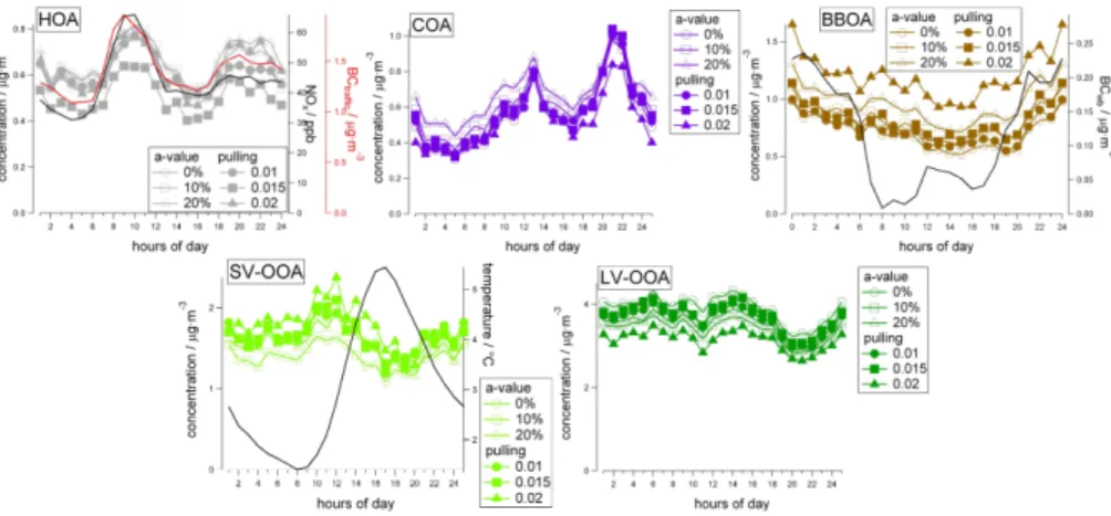
3.2.3 Comparison of factor time series

Diurnal cycles for the environmentally reasonable model solutions are shown in Fig. 6. In addition, NO_x and BC_tra_ffi_c are plotted together with HOA, while BC_wb is plotted with 15

BBOA.

The diurnal trends of HOA, NOx, and BCtra_fficare highly correlated. The diurnal cycle of the cooking factor COA manifests a strong peak during meal activities, similar to COA factors found in other source apportionment studies conducted on NR-PM1 data in other cities such as Barcelona (Mohr et al., 2012) or Paris (Crippa et al., 2013b). BBOA 20

is correlated with BC_{wood burning}and is highest at night, consistent with domestic heating activities and previous measurements in Zurich (Lanz et al., 2008). The diurnal cycle of SV-OOA is anticorrelated with temperature, suggesting that the factor represents semivolatile material which is influenced by temperature-driven partitioning whereas the diurnal cycle of LV-OOA does not show strong diurnal trends.

(19)

AMTD

6, 6409–6443, 2013

F. Canonaco et al.

Title Page

Tables Figures

◭ ◮

Back Close

Full Screen / Esc

Discussion

P

a

per

|

Dis

cussion

P

a

per

|

Discussion

P

a

per

|

Discussio

n

P

a

per

|

4 Discussion

4.1 Uncertainty in bilinear model results

As discussed in the previous section, the bilinear model analysis using constraints in Fsolved by the ME-2 engine yield a set of environmentally reasonable solutions which definitely improve the source apportionment. Note that the fully unconstrained PMF 5

run did not even fall into the range of environmentally acceptable solutions. While the constrained ME-2 solutions have many features in common, the reported profiles and mass concentrations differ (see Table 2, Figs. 5 and 6). This variation reflects the model uncertainty for the bilinear system. Rotational techniques, such as theavalue, pulling equations or individual rotations as well as the frequently used global rotational tool 10

fpeak are valuable tools for the quantitative assessment of the bilinear model uncer-tainty.

An additional source of uncertainty in the model results derives from the selection of the anchoring factor profiles and the magnitude of their constraints. The effects of the latter are evident from the CMB result (see Sect. 2.2.1). In particular, the mass 15

contribution of the SV-OOA factor was almost negligible. This occurred because the profiles were completely fixed, leaving the model with no chance to adapt the SV-OOA profile to the measured data. However, a semi-volatile fraction has been modeled for theavalue, pulling and even in the PMF approaches. This underlines the fact that if an anchor profile is too tight, a legitimate factor may be excluded from the model result. 20

The effect of choosing various factor profiles is highlighted by the comparison with the results of Lanz et al. (2008), in which winter AMS data from Zurich was analyzed using a constrained HOA factor profile with anavalue of 60 %. This value is consider-ably higher than the maximumavalue of 20 % selected in this study. The difference in the requiredavalue for these two studies is likely due to the choice of the HOA factor 25

profile. In the present study, the employed HOA anchor profile has a non-zero contribu-tion inm/z44 (1.4 %). Most probably, a largeavalue would lead to a mixing situation based on the variablem/z 44 which is avoided by using only smaller a values. This

(20)

AMTD

6, 6409–6443, 2013

F. Canonaco et al.

Title Page

Tables Figures

◭ ◮

Back Close

Full Screen / Esc

Discussion

P

a

per

|

Dis

cussion

P

a

per

|

Discussion

P

a

per

|

Discussio

n

P

a

per

|

was not the case in the constrained factor used in Lanz et al. (2008) as nom/z44 was present at all (0 %).

However, testing of the influence of different anchoring profiles and the tightness of their constraints, before a solution lacks in environmental interpretation, is ongoing and will be methodically discussed in a future study.

5

4.2 Recommendations for ME-2 analysis of aerosol mass spectra

Currently, there is very little experience regarding the inclusion of a priori information in the source apportionment for aerosol mass spectrometer data. The scope of this work is to facilitate the source apportionment in this respect by testing in a semi-automatic way different rotational tools of ME-2 with the graphical user interface SoFi.

10

Generally, the user can anchor factor information (profiles or time series) and easily vary the tightness of the constraint, while monitoring the various criteria for evaluation of a solution (see Sect. 2.2.7). Based on the experience gained in this study, for NR-PM₁source apportionments it is recommended to constrain the primary factors (HOA, COA, BBOA), whenever the PMF run reveals indications for such sources in the PMF 15

model result and or in the corresponding residuals. The secondary species can in first runs stay unconstrained, since they do not represent specific emissions rather span the range of aging processes in a specific location during the measurement time. Thus, it is difficult to match this evolution with auxiliary data. However, this topic is under study and more information will be provided in future.

20

The user should in any case perform sensitivity tests on the tightness of the con-straint (avalue or pulling parameters), to assess the environmentally reasonable solu-tions and present this range rather than only a single solution. As stated in Sect. 3.1, these parameters highly depend on the anchoring profiles employed and thus no limits for these values can be suggested at this stage. However, in general the increase of 25

(21)

AMTD

6, 6409–6443, 2013

F. Canonaco et al.

Title Page

Tables Figures

◭ ◮

Back Close

Full Screen / Esc

Discussion

P

a

per

|

Dis

cussion

P

a

per

|

Discussion

P

a

per

|

Discussio

n

P

a

per

|

Crippa et al. (2013) are performing the source apportionment with the ME-2 engine on the AMS EUCAARI data measured in 2008/2009, with the aim to standardize the method of source apportionment on NR-PM1data with ME-2 to some extend.

5 Conclusions

Source apportionment using the bilinear model as implemented through the multilin-5

ear engine (ME-2) was successfully applied to non-refractory organic aerosol (OA) mass spectra measured during winter 2011 and 2012 in Zurich, Switzerland using the aerosol chemical speciation monitor ACSM. The solutions were analyzed exploiting the newly developed source finder SoFi. The selected solution consists of two secondary factors and three primary factors. The secondary factors are a semi-volatile oxidized 10

OA (SV-OOA) and a low-volatility oxidized OA (LV-OOA). The three primary factors are traffic-related hydrocarbon-like OA (HOA), cooking OA (COA) and biomass burning OA (BBOA).

Different rotational approaches were investigated employing the ME-2 engine. The tested implementations consisted of (unconstrained matrix F and G) positive matrix 15

factorization (PMF), (fully constrained) chemical mass balance (CMB), and partially constrained models using theavalue parameter and pulling equations for the matrixF. In addition, for theavalue and pulling model runs a sensitivity test on the constrained profiles was performed. This allowed to identify the set of environmentally reasonable solutions.

20

Moreover, such analysis provides insight into the robustness and uncertainty of the bilinear model solution, e.g. the primary factor BBOA and the secondary semivolatile factor SV-OOA show the highest variability across models (implying the highest model uncertainty), while COA and HOA have the least variability (smallest model uncer-tainty).

25

Finally, some recommendations for future NR-PM₁source apportionments exploiting ME-2 are reported.

(22)

AMTD

6, 6409–6443, 2013

F. Canonaco et al.

Title Page

Tables Figures

◭ ◮

Back Close

Full Screen / Esc

Discussion

P

a

per

|

Dis

cussion

P

a

per

|

Discussion

P

a

per

|

Discussio

n

P

a

per

|

Supplementary material related to this article is available online at: http://www.atmos-meas-tech-discuss.net/6/6409/2013/

amtd-6-6409-2013-supplement.pdf.

Acknowledgements. The ACSM measurements were supported by the Swiss Federal Office for the Environment (FOEN). J. Slowik acknowledges support from the Swiss National Science

5

Foundation (SNF) through the “Ambizione” program. The authors would like to thank P. Paatero for the valuable comments during the analysis of the data and especially to the Environmental group of the Swiss Federal Laboratories for Materials and Testing (EMPA) for their support. Special thanks are also owed to Michele Canonaco for a critical reading of this manuscript.

References 10

Alfarra, M. R., Prevot, A. S. H., Szidat, S., Sandradewi, J., Weimer, S., Lanz, V. A., Schreiber, D., Mohr, M., and Baltensperger, U.: Identification of the mass spectral signature of organic aerosols from wood burning emissions, Environ. Sci. Technol., 41, 5770–5777, 2007. Allan, J. D., Alfarra, M. R., Bower, K. N., Williams, P. I., Gallagher, M. W., Jimenez, J. L.,

Mc-Donald, A. G., Nemitz, E., Canagaratna, M. R., Jayne, J. T., Coe, H., and Worsnop, D. R.:

15

Quantitative sampling using an Aerodyne aerosol mass spectrometer: 2. measurements of fine particulate chemical composition in two UK cities, J. Geophys. Res.-Atmos., 108, 4091, doi:10.1029/2002JD002359, 2003a.

Allan, J. D., Jimenez, J. L., Williams, P. I., Alfarra, M. R., Bower, K. N., Jayne, J. T., Coe, H., and Worsnop, D. R.: Quantitative sampling using an Aerodyne aerosol mass spectrometer:

20

1. Techniques of data interpretation and error analysis, J. Geophys. Res.-Atmos., 108, 4090, doi:10.1029/2002JD002358, 2003b.

Allan, J. D., Delia, A. E., Coe, H., Bower, K. N., Alfarra, M. R., Jimenez, J. L., Middlebrook, A. M., Drewnick, F., Onasch, T. B., Canagaratna, M. R., Jayne, J. T., and Worsnop, D. R.: A gener-alised method for the extraction of chemically resolved mass spectra from Aerodyne aerosol

25

mass spectrometer data, J. Aerosol Sci., 35, 909–922, 2004.

(23)

AMTD

6, 6409–6443, 2013

F. Canonaco et al.

Title Page

Tables Figures

◭ ◮

Back Close

Full Screen / Esc

Discussion

P

a

per

|

Dis

cussion

P

a

per

|

Discussion

P

a

per

|

Discussio

n

P

a

per

|

and cooking to primary organic aerosols in two UK cities, Atmos. Chem. Phys., 10, 647–668, doi:10.5194/acp-10-647-2010, 2010.

Amato, F. and Hopke, P. K.: Source apportionment of the ambient PM_2.5across St. Louis using constrained positive matrix factorization, Atmos. Environ., 46, 329–337, 2012.

Canagaratna, M. R., Jayne, J. T., Ghertner, D. A., Herndon, S., Shi, Q., Jimenez, J. L.,

5

Silva, P. J., Williams, P., Lanni, T., Drewnick, F., Demerjian, K. L., Kolb, C. E., and Worsnop, D. R.: Chase studies of particulate emissions from in-use New York City vehicles, Aerosol Sci. Tech., 38, 555–573, 2004.

Canagaratna, M. R., Jayne, J. T., Jimenez, J. L., Allan, J. D., Alfarra, M. R., Zhang, Q., Onasch, T. B., Drewnick, F., Coe, H., Middlebrook, A., Delia, A., Williams, L. R.,

Trim-10

born, A. M., Northway, M. J., DeCarlo, P. F., Kolb, C. E., Davidovits, P., and Worsnop, D. R.: Chemical and microphysical characterization of ambient aerosols with the Aerodyne aerosol mass spectrometer, Mass Spectrom. Rev., 26, 185–222, doi:10.1002/mas.20115, 2007. Crippa, M., DeCarlo, P. F., Slowik, J. G., Mohr, C., Heringa, M. F., Chirico, R., Poulain, L.,

Freutel, F., Sciare, J., Cozic, J., Di Marco, C. F., Elsasser, M., Nicolas, J. B., Marchand, N.,

15

Abidi, E., Wiedensohler, A., Drewnick, F., Schneider, J., Borrmann, S., Nemitz, E., Zimmer-mann, R., Jaffrezo, J.-L., Pr ´ev ˆot, A. S. H., and Baltensperger, U.: Wintertime aerosol chemi-cal composition and source apportionment of the organic fraction in the metropolitan area of Paris, Atmos. Chem. Phys., 13, 961–981, doi:10.5194/acp-13-961-2013, 2013a.

Crippa, M., Canonaco, F., Prevot, A. S. H., and Baltensperger, U.: A compilation of organic

20

aerosol components for AMS datasets across Europe using a newly developed ME-2 based source apportionment strategy, in preparation, 2013b.

Empa: Technischer Bericht zum Nationalen Beobachtungsnetz f ¨ur Luftfremdstoffe (NABEL), available at: http://www.empa.ch (last access: 11 July 2013), 2011.

Hallquist, M., Wenger, J. C., Baltensperger, U., Rudich, Y., Simpson, D., Claeys, M.,

Dom-25

men, J., Donahue, N. M., George, C., Goldstein, A. H., Hamilton, J. F., Herrmann, H., Hoff -mann, T., Iinuma, Y., Jang, M., Jenkin, M. E., Jimenez, J. L., Kiendler-Scharr, A., Maen-haut, W., McFiggans, G., Mentel, Th. F., Monod, A., Pr ´ev ˆot, A. S. H., Seinfeld, J. H., Sur-ratt, J. D., Szmigielski, R., and Wildt, J.: The formation, properties and impact of sec-ondary organic aerosol: current and emerging issues, Atmos. Chem. Phys., 9, 5155–5236,

30

doi:10.5194/acp-9-5155-2009, 2009.

He, L.-Y., Lin, Y., Huang, X.-F., Guo, S., Xue, L., Su, Q., Hu, M., Luan, S.-J., and Zhang, Y.-H.: Characterization of high-resolution aerosol mass spectra of primary organic aerosol

(24)

AMTD

6, 6409–6443, 2013

F. Canonaco et al.

Title Page

Tables Figures

◭ ◮

Back Close

Full Screen / Esc

Discussion

P

a

per

|

Dis

cussion

P

a

per

|

Discussion

P

a

per

|

Discussio

n

P

a

per

|

sions from Chinese cooking and biomass burning, Atmos. Chem. Phys., 10, 11535–11543, doi:10.5194/acp-10-11535-2010, 2010.

Herich, H., Hueglin, C., and Buchmann, B.: A 2.5 year’s source apportionment study of black carbon from wood burning and fossil fuel combustion at urban and rural sites in Switzerland, Atmos. Meas. Tech., 4, 1409–1420, doi:10.5194/amt-4-1409-2011, 2011.

5

IPCC: IPCC Fourth Assessment Report: The Physical Science Basis, Working Group I, Final Report, Geneva, Switzerland, 2007.

Jayne, J. T., Leard, D. C., Zhang, X. F., Davidovits, P., Smith, K. A., Kolb, C. E., and Worsnop, D. R.: Development of an aerosol mass spectrometer for size and composition analysis of submicron particles, Aerosol Sci. Tech., 33, 49–70, 2000.

10

Jimenez, J. L., Jayne, J. T., Shi, Q., Kolb, C. E., Worsnop, D. R., Yourshaw, I., Seinfeld, J. H., Flagan, R. C., Zhang, X. F., Smith, K. A., Morris, J. W., and Davidovits, P.: Ambient aerosol sampling using the Aerodyne aerosol mass spectrometer, J. Geophys. Res.-Atmos., 108, 8425, doi:10.1029/2001JD001213, 2003.

Jimenez, J. L., Canagaratna, M. R., Donahue, N. M., Prevot, A. S. H., Zhang, Q., Kroll, J. H.,

15

DeCarlo, P. F., Allan, J. D., Coe, H., Ng, N. L., Aiken, A. C., Docherty, K. S., Ulbrich, I. M., Grieshop, A. P., Robinson, A. L., Duplissy, J., Smith, J. D., Wilson, K. R., Lanz, V. A., Hueglin, C., Sun, Y. L., Tian, J., Laaksonen, A., Raatikainen, T., Rautiainen, J., Vaatto-vaara, P., Ehn, M., Kulmala, M., Tomlinson, J. M., Collins, D. R., Cubison, M. J., Dunlea, E. J., Huffman, J. A., Onasch, T. B., Alfarra, M. R., Williams, P. I., Bower, K., Kondo, Y.,

Schnei-20

der, J., Drewnick, F., Borrmann, S., Weimer, S., Demerjian, K., Salcedo, D., Cottrell, L., Grif-fin, R., Takami, A., Miyoshi, T., Hatakeyama, S., Shimono, A., Sun, J. Y., Zhang, Y. M., Dzepina, K., Kimmel, J. R., Sueper, D., Jayne, J. T., Herndon, S. C., Trimborn, A. M., Williams, L. R., Wood, E. C., Middlebrook, A. M., Kolb, C. E., Baltensperger, U., and Worsnop, D. R.: Evolution of organic aerosols in the atmosphere, Science, 326, 1525–1529,

25

2009.

Khaykin, S. M., Pommereau, J.-P., and Hauchecorne, A.: Impact of land convection on the thermal structure of the lower stratosphere as inferred from COSMIC GPS radio occultations, Atmos. Chem. Phys. Discuss., 13, 1–31, doi:10.5194/acpd-13-1-2013, 2013a.

Lanz, V. A., Alfarra, M. R., Baltensperger, U., Buchmann, B., Hueglin, C., and Pr ´ev ˆot, A. S. H.:

30

(25)

AMTD

6, 6409–6443, 2013

F. Canonaco et al.

Title Page

Tables Figures

◭ ◮

Back Close

Full Screen / Esc

Discussion

P

a

per

|

Dis

cussion

P

a

per

|

Discussion

P

a

per

|

Discussio

n

P

a

per

|

Lanz, V. A., Alfarra, M. R., Baltensperger, U., Buchmann, B., Hueglin, C., Szidat, S., Wehrli, M. N., Wacker, L., Weimer, S., Caseiro, A., Puxbaum, H., and Prevot, A. S. H.: Source attribution of submicron organic aerosols during wintertime inversions by ad-vanced factor analysis of aerosol mass spectra, Environ. Sci. Technol., 42, 214–220, doi:10.1021/es0707207, 2008.

5

Lanz, V. A., Pr ´ev ˆot, A. S. H., Alfarra, M. R., Weimer, S., Mohr, C., DeCarlo, P. F., Gianini, M. F. D., Hueglin, C., Schneider, J., Favez, O., D’Anna, B., George, C., and Baltensperger, U.: Char-acterization of aerosol chemical composition with aerosol mass spectrometry in Central Eu-rope: an overview, Atmos. Chem. Phys., 10, 10453–10471, doi:10.5194/acp-10-10453-2010, 2010.

10

Matson, P., Lohse, K. A., and Hall, S. J.: The globalization of nitrogen deposition: consequences for terrestrial ecosystems, Ambio, 31, 113–119, 2002.

Matthew, B. M., Middlebrook, A. M., and Onasch, T. B.: Collection e_fficiencies in an Aerodyne aerosol mass spectrometer as a function of particle phase for laboratory generated aerosols, Aerosol Sci. Tech., 42, 884–898, doi:10.1080/02786820802356797, 2008.

15

Middlebrook, A. M., Bahreini, R., Jimenez, J. L., and Canagaratna, M. R.: Evaluation of composition-dependent collection efficiencies for the Aerodyne aerosol mass spectrome-ter using field data, Aerosol Sci. Tech., 46, 258–271, doi:10.1080/02786826.2011.620041, 2012.

Mohr, C., DeCarlo, P. F., Heringa, M. F., Chirico, R., Slowik, J. G., Richter, R., Reche, C.,

20

Alastuey, A., Querol, X., Seco, R., Pe ñuelas, J., Jim énez, J. L., Crippa, M., Zimmermann, R., Baltensperger, U., and Pr év ôt, A. S. H.: Identification and quantification of organic aerosol from cooking and other sources in Barcelona using aerosol mass spectrometer data, Atmos. Chem. Phys., 12, 1649–1665, doi:10.5194/acp-12-1649-2012, 2012.

Ng, N. L., Canagaratna, M. R., Jimenez, J. L., Zhang, Q., Ulbrich, I. M., and Worsnop, D. R.:

25

Real-time methods for estimating organic component mass concentrations from aerosol mass spectrometer data, Environ. Sci. Technol., 45, 910–916, doi:10.1021/es102951k, 2011a.

Ng, N. L., Herndon, S. C., Trimborn, A., Canagaratna, M. R., Croteau, P. L., Onasch, T. B., Sueper, D., Worsnop, D. R., Zhang, Q., Sun, Y. L., and Jayne, J. T.: An aerosol chemical

spe-30

ciation monitor (ACSM) for routine monitoring of the composition and mass concentrations of ambient aerosol, Aerosol Sci. Tech., 45, 770–784, doi:10.1080/02786826.2011.560211, 2011b.

(26)

AMTD

6, 6409–6443, 2013

F. Canonaco et al.

Title Page

Tables Figures

◭ ◮

Back Close

Full Screen / Esc

Discussion

P

a

per

|

Dis

cussion

P

a

per

|

Discussion

P

a

per

|

Discussio

n

P

a

per

|

Paatero, P.: Least squares formulation of robust non-negative factor analysis, Chemometr. Intell. Lab., 37, 23–35, 1997.

Paatero, P.: The multilinear engine – a table-driven, least squares program for solving multilinear problems, including the n-way parallel factor analysis model, J. Comput. Graph. Stat., 8, 854– 888, 1999.

5

Paatero, P.: User’s Guide for Positive Matrix Factorization Programs PMF2 and PMF3, Univer-sity of Helsinki, Finland, 2007.

Paatero, P. and Tapper, U.: Analysis of different modes of factor analysis as least squares fit problems, Chemometr. Intell. Lab., 18, 183–194, 1993.

Paatero, P. and Tapper, U.: Positive matrix factorization – a nonnegative factor model with

opti-10

mal utilization of error-estimates of data values, Environmetrics, 5, 111–126, 1994.

Paatero, P., Hopke, P. K., Song, X. H., and Ramadan, Z.: Understanding and controlling rota-tions in factor analytic models, Chemometr. Intell. Lab., 60, 253–264, 2002.

Paatero, P. and Hopke, P. K.: Rotational tools for factor analytic models, J. Chemometr., 23, 91–100, 2009.

15

Peng, R. D., Dominici, F., Pastor-Barriuso, R., Zeger, S. L., and Samet, J. M.: Seasonal analyses of air pollution and mortality in 100 US cities, Am. J. Epidemiol., 161, 585–594, doi:10.1093/aje/kwi075, 2005.

Reche, C., Viana, M., Amato, F., Alastuey, A., Moreno, T., Hillamo, R., Teinila, K., Saarnio, K., Seco, R., Penuelas, J., Mohr, C., Prevot, A. S. H., and Querol, X.: Biomass burning

contribu-20

tions to urban aerosols in a coastal Mediterranean City, Sci. Total. Environ., 427, 175–190, doi:10.1016/j.scitotenv.2012.04.012, 2012.

Sandradewi, J., Prevot, A. S. H., Szidat, S., Perron, N., Alfarra, M. R., Lanz, V. A., Weingart-ner, E., and Baltensperger, U.: Using aerosol light absorption measurements for the quanti-tative determination of wood burning and traffic emission contributions to particulate matter,

25

Environ. Sci. Techol., 42, 3316–3323, doi:10.1021/es702253m, 2008.

Slowik, J. G., Vlasenko, A., McGuire, M., Evans, G. J., and Abbatt, J. P. D.: Simultaneous factor analysis of organic particle and gas mass spectra: AMS and PTR-MS measurements at an urban site, Atmos. Chem. Phys., 10, 1969–1988, doi:10.5194/acp-10-1969-2010, 2010. Sun, Y.-L., Zhang, Q., Schwab, J. J., Demerjian, K. L., Chen, W.-N., Bae, M.-S., Hung, H.-M.,

30

(27)

time-of-AMTD

6, 6409–6443, 2013

F. Canonaco et al.

Title Page

Tables Figures

◭ ◮

Back Close

Full Screen / Esc

Discussion

P

a

per

|

Dis

cussion

P

a

per

|

Discussion

P

a

per

|

Discussio

n

P

a

per

|

flight aerosol mass apectrometer, Atmos. Chem. Phys., 11, 1581–1602, doi:10.5194/acp-11-1581-2011, 2011.

Ulbrich, I. M., Canagaratna, M. R., Zhang, Q., Worsnop, D. R., and Jimenez, J. L.: Interpretation of organic components from positive matrix factorization of aerosol mass spectrometric data, Atmos. Chem. Phys., 9, 2891–2918, doi:10.5194/acp-9-2891-2009, 2009.

5

Watson, J. G.: Visibility: science and regulation, JAPCA J. Air Waste Manage., 52, 628–713, doi:10.1080/10473289.2002.10470813, 2002.

Wold, S., Esbensen, K., and Geladi, P.: Principal component analysis, Chemometr. Intell. Lab., 2, 37–52, doi:10.1016/0169-7439(87)80084-9, 1987.

Zhang, Q., Alfarra, M. R., Worsnop, D. R., Allan, J. D., Coe, H., Canagaratna, M. R., and

10

Jimenez, J. L.: Deconvolution and quantification of hydrocarbon-like and oxygenated or-ganic aerosols based on aerosol mass spectrometry, Environ. Sci. Technol., 39, 4938–4952, doi:10.1021/es048568l, 2005.

Zhang, Q., Jimenez, J. L., Canagaratna, M. R., Ulbrich, I. M., Ng, N. L., Worsnop, D. R., and Sun, Y.: Understanding atmospheric organic aerosols via factor analysis of aerosol mass

15

spectrometry: a review, Anal. Bioanal. Chem., 401, 3045–3067, doi:10.1007/s00216-011-5355-y, 2011.