Ion composition measurements and modelling at altitudes
from 140 to 350 km using EISCAT measurements
A. Litvine, W. Kofman, B. Cabrit
Centre d'Etude des PheÂnomeÁnes AleÂatoires et GeÂophysiques, B.P. 46, F-38402 Saint Martin d'HeÁres, France Fax: +33 04 76 82 63 84; e-mail: wlodek. [email protected]
Received: 6 November 1997 / Revised: 3 February 1998 / Accepted: 16 March 1998
Abstract. This work aims at processing the data of CP1 and CP2 programs of EISCAT ionospheric radar from 1987 to 1994 using the ``full pro®le'' method which allows to solve the ``temperature-composition'' ambigu-ity problem in the lower F region. The program of data analysis was developed in the CEPHAG in 1995±1996. To improve this program, we implemented another analytical function to model the ion composition pro®le. This new function better re¯ects the real pro®le of the composition. Secondly, we chose the best method to select the initial conditions for the ``full pro®le'' proce-dure. A statistical analysis of the results was made to obtain the averages of various parameters: electron concentration and temperature, ion temperature, com-position and bulk velocity. The aim is to obtain models of the parameter behaviour de®ning the ion composition pro®les : z50 (transition altitude between atomic and molecular ions) and dz(width of the pro®le), for various seasons and for high and low solar activities. These models are then compared to other models. To explain the principal features of parametersz50anddz, we made an analysis of the processes leading to composition changes and related them to production and electron density pro®le. A new experimental model of ion composition is now available.
Key words. Auroral ionosphere Ion chemistry and composition Instruments and techniques
EISCAT
1 Introduction
The ion composition analysis in the F region is one of the most dicult problems in incoherent-scatter data analysis. In the F ionospheric region, between about 140
and 350 km, the transition between molecular and atomic ion composition occurs. This transition region varies depending on the geophysical conditions, and this is especially important for the auroral region, where the in¯uence of energy inputs is large.
The incoherent-scatter spectrum depends on ®ve parameters in this region:
ne: electron density,
Teand Ti: electron and ion temperature, p: ion composition,
vi: ion velocity,
but the determination of ®ve parameters simultaneously is very dicult, strongly depending on the signal-to-noise ratio and the method of measurements. For these reasons, one of the parameters, usually the ion compo-sition, is ®xed by the model. However, one can otherwise model the ion temperature by the Bates pro®le plus a correction term and model the ion composition (Oliver, 1979) and determine parameters. Dierent approaches were developed in order to derive the ion composition. This study was started at the beginning of incoherent-scatter work by Petit (1963) and Moorcroft (1964) and then improved by LathuilleÁreet al. (1983).
The analysis proposed by LathuilleÁre et al. (1983) consists in the determination of ®ve parameters simulta-neously. This is possible if the initial values chosen for the ®t are not too far from the solution, and the data are integrated long enough. The method used to ®nd the initial values consisted in making several ®ts on the measured ACF with a ®xed composition ranging from only molecular ions to Oions. The results of the ®t for each assumed composition are the ionospheric parame-ters and the reduced square parameter. The chi-square parameter is the reduced quadratic errors between the ®t and the measured ACF and is usually used to check the quality of the ®t. The parameters corresponding to the minimum value of chi-square are the closest ones to the solution and are chosen as initial values. Then a new ®t was performed on all parameters including the compo-sition. Each altitude is analysed independently.
There is an additional diculty arising from the fact that there are often two minima in chi-square, very close to each other and occurring for composition values approximately symmetrical with respect to 0.5. So when minima were found, the two corresponding sets of initial values were used for the ®nal ®t and two possible values of composition were obtained for each ACF. The choice between these two sets of data was made afterwards, when all ACFs corresponding to all altitudes were reduced: one chooses the composition values when the pro®le ®ts the smoothest curve between 0 and 1 among all the possibilities. This processing strongly depends on the signal-to-noise ratio; the results are noisy and need averaging over a period of a few hours.
This method was applied on a few years of data (LathuilleÁre and Pibaret, 1992) and the authors deter-mined a model of ion composition, especially for the altitude of the transition z50) between 50% of molecular and oxygen ions. In the last 5 years, several improve-ments in incoherent-scatter data analysis have occurred; see Holtet al. (1992), Lehtinenet al. (1996), Cabrit and Kofman (1996). All these works are based on the ``full pro®le'' approach which consists in ®tting the whole set of scatter measurements at one time. This new analysis technique was proved to be the best possible way of reaching spatial resolution by directly ®tting the set of lag pro®les. It also has the advantage of leading to plasma parameters free from the gradient eects which usually corrupt standard analysis results (Holt et al. (1992).
In Cabrit and Kofman (1996) it was shown that the ``full pro®le'' technique can be eciently used to extract independent information on the ion composition and on the ion temperature from incoherent-scatter data. The implementation was designed for EISCAT CP1 and CP2 data analysis. This means that ®tted data are the gated lag pro®le cross-products, namely the plasma correla-tion funccorrela-tions. The ®rst key point in Cabrit and Kofman's method is that one has to ®t simultaneously high-resolution/low-signal (coded-pulse) and low-reso-lution/high-signal (long-pulse) data. The second key point is that one needs a suitable functional model of ion composition pro®le with a sucient amount of ¯exibil-ity to include all possible variations. The model used in the present study is dierent from the one presented in Cabrit and Kofman (1996). It will be described in the next chapter.
As we wanted to analyse the data measured by EISCAT over about 7 years, we had to automate the analysis in order to be able to do it relatively fast. As previous authors, we introduced two parameters signif-icantly describing the composition pro®le; the z50 parameters corresponding to the transition region between 50% of molecular and atomic ions and the width dz of the transition de®ned in this paper as the altitude width between 10% and 90% of the composi-tion. We studied the seasonal behaviour of the compo-sition; the results of our analyses are shown and described precisely.
In the introduction, we want to emphasise the interesting behaviour, still needing a detailed
explana-tion, of the z50 and dz parameters. z50 and dz show anticorrelation in summer and correlation in winter. This means that whenz50decreases, dzalso decreases in winter and dz has the opposite behaviour in summer. From our data, spring and autumn are transition periods between these two opposite behaviours.
The analysis of a large amount of data allows us to present two seasonal models for low and high solar activity for geophysical conditions without electric ®eld in the ®eld of view of the radar. The data analysis for perturbed geophysical conditions is much more dicult and still under study (Gaimardet al., 1998). In fact, for high convection electric ®elds, the ion velocity distribu-tion is no longer Maxwellian (Saint Maurice and Schunk, 1979; Hubert and Kinzelin, 1992) and this basic assumption in the data analysis is not valid. In addition, during high auroral activity, the fast time variability of the parameters prevents long integration time.
Our experimental model is important as an input to the polar ionospheric data bank, especially as this kind of data is very sparse. There are very few data concerning the ion composition because the satellite measurements in the F1 region of the ionosphere are dicult and rare.
2 Data analysis
2.1 Functional model of ionospheric parameters
In our work we use the technique of ``full pro®le'' analysis which needs modelling, as a function of altitude, of the ionospheric parametersne, Te,Ti,p and vi by functions depending on a few parameters. The method used is fully described in Cabrit and Kofman (1996). Here we brie¯y sum up the main features. In order to solve the inversion problem, we model the four basic parameters by cubic spline functions. The ion composition is modelled using the method of Oliver (1979). This function is close to the analytical model used by Cabrit and Kofman (1996) and to the model established by LathuilleÁre and Pibaret (1992). The ``full pro®le'' procedure performs a parametric optimisation of the model parameters in the least-square sense.
The model of Cabrit and Kofman (1996) is purely an analytical one, built in order to approximate the IRI and LathuilleÁre and Pibaret (1992) models, the latter being obtained from previous EISCAT measurements and modelled by the hyperbolic tangent function. In Oliver's work, the model was based on a physical consideration using the continuity equation in a steady state. Oliver (1979) showed that the ion molecular composition can be well approximated by the following formula:
p1ÿ 2
1 q1 n z8 n z 50exp t050 PP zz50ÿ1
; 1
the density of the hypothetical neutral component and P(z) is its pressure.
Instead of using a component with an hypothetical mass, we used the mean neutral density according to the formula:
n z n016 n0232 nN228
76 : 2
The pressure was calculated by P z n z kT z. In order to simplify our model, which cannot depend on too many parameters, we used the hydrostatic equation for the neutral densities.
n z n0 T0 T zexp
ÿ
Zz
z0
dz1 H z 1
; 3
H z kT z
mg ± the scale height;
and for neutral temperatures the Bates pro®le
T z T1 ÿ T1 ÿT0exp ÿs z ÿ z0 ; 4 wherez0= 100 km,n0± the neutral density atz0,T0± the temperature, m is the mass of the neutral component and kis Boltzman's constant.
In our model we tookn0 from the MSIS 90 model: T1 = 900 K, T0 = 200 K and s= 0.03. These values
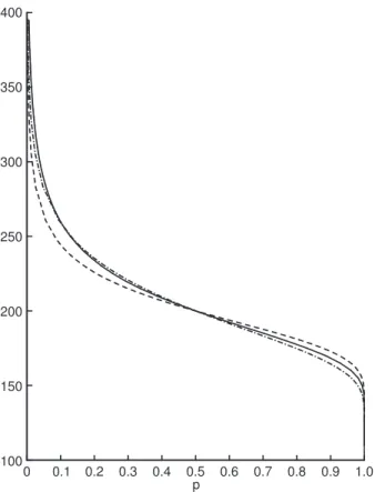
were chosen to be as close as possible to the neutral atmosphere given by MSIS 90, but of course the pro®les obtained with the hydrostatic Eq. (3) are quite dierent from the pro®les given by the MSIS model. The dierence between the ion composition pro®lep(z) given by Eq. (1), in which the neutral atmosphere is given by Eqs. (2), (3) and (4) andp(z) calculated with the neutral atmosphere obtained with the MSIS 90 model is shown in Fig. 1. We plot in a continuous line the ion composition pro®le obtained with the MSIS 90 model with z50=200 km and t050=1.5, and two pro®les using approximating formulas for the neutral component with z50=200 km and t050=1.5 and 0.8. One can see that the curve for t050=0.8 is close to the one using the MSIS 90 model. The plots clearly show that our modelling is adequate. Therefore, in our analysis we use Eqs. (1)±(4).
Oliver's model was derived for daytime photochem-ical equilibrium conditions. The applicability of this model for night-time conditions is not demonstrated. We use this model because the functional form is close to previously used models (LathuilleÁre and Pibaret, 1992, Cabrit and Kofman, 1996) and there is a theoret-ical justi®cation for sunny atmosphere. In addition, during night conditions, precipitations produce ionisat-ion. In particular, the physical sense of thet050 param-eter during the night is only related to the width of the pro®le and not to the optical depth.
100 150 200 250 300 350 400
1.0 0.9 0.8 0.7 0.6 0.5 0.4 0.3 0.2 0.1 0
p
Fig. 1. The ion composition pro®lep z 1ÿO
ne calculated by Eq.
(1), using the neutral atmosphere from the MSIS 90 model (continuous lines) and z50=200, t050=1.5, and our modelling for z50=200,
t050=1.5 (dotted lines) andz50=200,t050=0.8 (dash-dotted lines)
Winter
Low solar activity: F10.7<125 Summer Autumn Spring
High solar activity: F10.7>125
0
0 20
20 40
40 60
60 80
80 100
100 120
120 140
140 160
160
94
94 93
93 92
92 91
91 90
90 89
89 88 87
Year
Year
Number of hours
Number of hours
2.2 Initial conditions for the ®t
In order to process a large amount of data, one had to solve the following problem: how to ®nd the correct initial values. Simulations show that, with the functional dependence of the composition we are using, there is only one minimum of the mean quadratic error between the parametric data model and synthetic data. This is basically dierent from the existence of two minima in the classical gate-by-gate least-square ®tting discussed in the introduction (see also Fig. 1 in LathuilleÁre and Pibaret, 1992). Actually, when one uses real data, there
are rather often two local minima, especially during the night period when the signal-to-noise ratio is small. This anomalous behaviour is due to a few technical reasons: the adjustment (calibration) between the various types of correlation function measurements (long-pulse ± multi-pulse or long-pulse ± alternating code) or the approximation used in the ambiguity function calcula-tion which assumes the ideal rectangular transmitted impulse and the constant gain may not be precise enough. Depending on the initial conditions, the ®t converges on one or the other solution (local minimum). Hopefully, one of these solutions can be rejected because
0 0
0 0
50 50
50 50
100 100
100 100
150 150
150 150
200 200
200 200
250 250
250 250
300 300
300 300
20 20
20 20
15 15
15 15
10 10
10 10
5 5
5 5
0 0
0 0
Time (h) Time (h)
Time (h) Time (h)
zD
z
50
(km),
(km)
zD
z
50
(km),
(km)
zD
z
50
(km),
(km)
zD
z
50
(km),
(km)
Summer Autumn
Spring Winter
it corresponds to non-monotonic electron and ion temperature pro®les, which is unacceptable for data gathered during quiet ionospheric conditions. The other solution corresponds to smooth pro®les and is consid-ered to be the correct one.
For the automatic analysis of large amounts of data, we used the following strategy to select the ``correct'' solution:
1. One starts with ®xed initial conditions z50 = 200 and t050 = 0.5).
2. If the results of dz are smaller than the value of 125 km, and the ®t quality, which is the sum of the
quadratic distance between measured and theoretical ACFs normalised by variances of each lag (see Cabrit and Kofman, 1996) is less than 1.5 and errors on the parameters are smaller than 30%, the results are taken as de®nitive. If not, the analysis is restarted with z50 increased and decreased by steps of 10 km andt050=1.5.
3. If the results are correct, the values are used as initial conditions for the next ®t. If not, one starts with the ®xed initial conditions de®ned in point 1.
At the end of the analysis, the data are synthesised, and if one ®nds z50 at too low altitudes for a long-time
interval or Ti pro®le with non-monotonic behaviour for many hours, we restart the analysis changing the initial conditions and using the daily model of LathuilleÁre and Pibaret (1992) for z50 and t050= 1.5. Because of these diculties, we had to reanalyse about one half of the data for high solar activity periods. It is clear that we should avoid using the ®xed model for the initial
conditions to diminish the possibility of in¯uence of the model on the results. We performed the statistical analysis of the data twice: once using all the results, and once excluding the results which were obtained with the initial conditions from the model. The results of the statistical analysis were the same.
Fig. 5. The results of ®tting for various seasons and high (dashed line) and low (continuous line) solar activity are shown. The crossed line
corresponds to LathuilleÁre and Pibaret's model (there is no model for
spring). Thedash-dottedline corresponds to the IRI model for 100
2.3 Statistical analysis
We analysed a large amount of EISCAT data dating from 1987 to 1994. The CP1 and CP2 data were analysed with the multi-pulse and long-pulse, and alternating code and long-pulse measurement tech-niques. The data were split into two sets, one corre-sponding to high solar activity withF10:7>125 and the other to low solar activity for F10:7<125. The data were selected as a function of the seasons; winter and summer were de®ned as 2 months before and 2 months after the solstices and spring and autumn as 1 month before and one after the equinoxes. This season de®nition is identical to the one made by LathuilleÁre and Pibaret (1992). This choice is also justi®ed by the solar zenith angle variability during the various seasons. However, the choice of the season duration leads to a smaller amount of data for spring and au-tumn.
In Fig. 2 we show the histogram of analysed data for high and low solar activity. The aim of the statistical analysis is to obtain the average model of ion compo-sition for each season as a function of UT. The averaged data were ®tted with the fourth-order polynomial with continuity conditions on the polynomial and its deriv-atives at 0 UT. We also averaged the other ionospheric parameters ne,Te,Ti andvi.
As we explained before, we have only built the model for geophysical conditions without large electric ®eld. In order to do so, we had to eliminate the data corre-sponding to periods of large electric ®eld, larger than 25 mV/m. For a larger electric ®eld, the ion velocity distribution starts to be non-Maxwellian and the anal-ysis is no longer valid (Saint Maurice and Schunk, 1979; Gaimard et al., 1996). When measurements of the electric ®eld were not available, we used the ion temperature at 130 km as a selection criterion. The large ion temperature at 130 km indicates the Joule heating present in the ionosphere and through this the presence of the electric ®eld. When the ion temperature was larger than 700 K, we rejected the data.
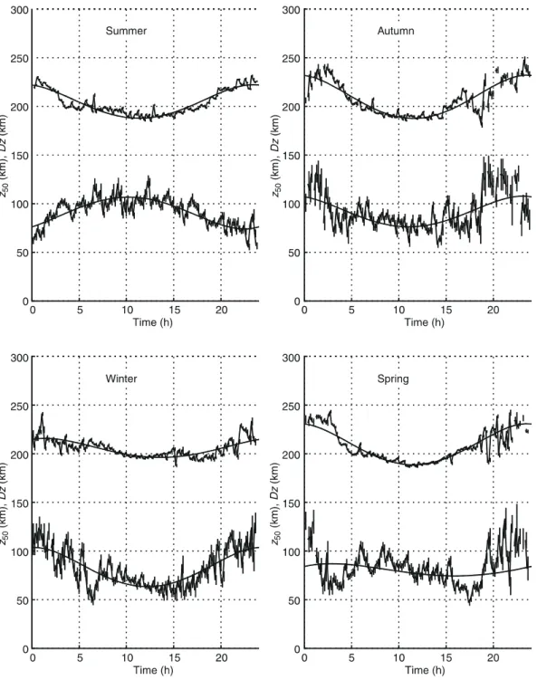
Once the data were selected, they were gathered in bins of 10 min as a function of the time (UT) for each season separately. The averages for all parameters z50, dz, ne, Ti, Te and vi were calculated. The weighted averages were made. The z50, dz and t050 parameters were ®tted by the polynomial as we explained before. In Figs. 3 and 4, we show the z50, and dz parameters for four seasons for low and high solar activity. The averaged points with their errors are shown with a 10-min time-resolution. The continuous lines correspond to the polynomial ®t. The most striking feature is the correlation and the anti-correlation of two parameters
z50 and dz) as a function of time. In summer, the two parameters are anticorrelated and in winter they are correlated. This behaviour is the same for high and low activity. The transition between these two behaviours is clearly seen for spring, but is weaker for autumn. For all seasons, one observes the minimum of the parameterz50 at about noon. This was observed in the paper by LathuilleÁre and Pibaret (1992). The amplitude of the
daily variation is smaller in winter and the minimum for winter is shifted by 2±3 h to the afternoon. The minimum of z50 is at about 180 km for F10:7<125 and at about 200 km forF10:7>125. For autumn, the behaviour of the measurements is opposite to their behaviour for winter: z50 is minimum at about 200 km for F10:7<125 and at about 190 km for F10:7>125. For summer and spring, there are no large dierences for the altitude of the minima for low and high solar activity.
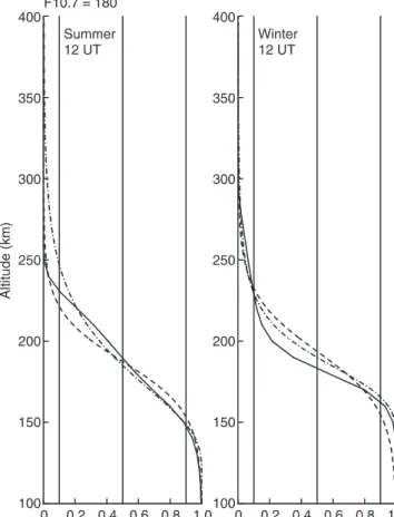
We gathered the results for low and high solar activity and compared them with those of the IRI model and LathuilleÁre and Pibaret (1992). In Fig. 5 we plotted (crosses)z50and dzobtained by LathuilleÁre and Pibaret (1992) compared to our results. In general, the z50 parameters show the same form. The striking feature is that our modelling corresponding toF10:7<125 (con-tinuous line) is close to the modelling of LathuilleÁre and Pibaret (1992) for summer and the modelling corre-sponding to F10:7>125 (dashed line) is close to LathuilleÁre and Pibaret's one for autumn. The reason is that the measurements analysed in LathuilleÁre and Pibaret (1992) are averaged independently on the solar activity and the distribution of these measurements is not uniform. What happened is that there were more data during low solar activity for summer (about twice the amount of data used in averaging coming from low activity than from high activity) and about the same amount of data during high and low solar activity for autumn (private communication from Pibaret). The width (dz) of the pro®les was analysed by LathuilleÁre and Pibaret globally, all data together. The authors searched for a linear dependence of the width (dz) onz50, and this is why dzhas the same form for all seasons, like z50 (except for spring, where there are no data). There are dierences with our results especially for summer. The overall behaviour is dierent. We think that this is due to two reasons. The ®rst is that all seasons were mixed and analysed together to ®nd a linear dependence between dzandz50(the data are very scattered, see Fig. 9 in LathuilleÁre and Pibaret). The second is that Lath-uilleÁre and Pibaret (1992) used plasma parameters inferred from a coarse-resolution (40 km), long-pulse data. Since the width of the transition region between molecular and atomic ions is of the same order as the spatial resolution, one can have some doubts regarding the behaviour of dz. In Fig. 6, we compare our pro®le obtained with Oliver's approximation (1979) with the pro®le of LathuilleÁre and Pibaret (1992) and the pro®le of the IRI model. This ®gure shows that LathuilleÁre and Pibaret's model and the results of this paper are dierent, especially for summer. This re¯ects the pre-vious discussion. The behaviour of LathuilleÁre and Pibaret's model for altitudes underz50is determined by assumed symmetry. In fact, there are no measurements (or few) for these altitudes in their modelling due to the use of long-pulse data.
the constant of z50 and dz as a function of time for winter, which is clearly dierent from our measure-ments.
In Table 1 (see Appendix), we give the coecients of the ®tted parameters (z50,t050and dz) of the fourth-order polynomial:
P t f1 f2 t 12
f3 t 12 2
f4 t 12 3
f5 t 12 4
with t ranging from 0 to 24. This table allows the generation of the model and its implementation.
3 Discussion of results
Some of the general characteristics of the temporal and seasonal behaviour described in the previous section can easily be explained with the simpli®ed steady-state model of chemical reactions in the F1 region of the ionosphere. The presence of the minimum of the transition altitude (z50) between molecular and O at noon has two main causes.
The increase in electron density due to the decrease in the solar zenith angle will act on two reactions (O+ N2!NO + N, NO + e !N + O). The rate of the ®rst one is proportional to the electron density, while the rate of the second one increases with its square.
Therefore, for a given altitude, when the electron density increases, the density of NOdecreases comparatively to Odensity and the result is the decrease inz50.
The second cause of the decrease inz50is the increase in the O/N2 ratio for all seasons at noon. In Fig. 7 we plot this ratio as a function of the altitude obtained from the MSIS 90 model. This increase will change the rate of ionisation of the atomic oxygen comparatively to the reaction O+ N
2 ! NO + N, and this will increase the relative ratio between Oand NO. In addition, the
increase in the O/N2 ratio modi®es the abundance of NO via the ionisation of N2 and the reaction N2 O!NO+ N, because the last reaction is the major loss for N2 ions and the major source for NO.
The observed decrease in the altitude minimum ofz50 in winter for low solar activity comparative to high solar activity can also be explained by the behaviour of the O/N2 ratio. The O/N2 ratio at 200 km for low solar activity is larger than for high solar activity at noon and this is why the altitude of the minimum increases for high solar activity.
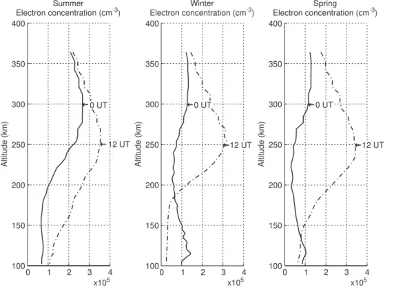
It is much more dicult to explain in a simple way the daily behaviour of the width of the ion composition pro®le dz. As we said before, we created an average model of measured ionospheric parameters according to seasons. In Fig. 8, we show the pro®les of electron density for three seasons. To discuss the variability of dz, we will use these pro®les. For winter, the decrease in dz in the middle of the day means that the changes in the ionosphere are faster when altitude increases. This implies that the gradients of the ionospheric parameters which make the transition to O should be stronger.
The major ionospheric parameters which in¯uence this transition are, as stated in the foregoing discussion, the electron density and the ratio of O/N2. In Fig. 8 we can see that for winter conditions, the electron density increases very fast at noon and at midnight the gradient is even negative at altitudes of interest. The fact that the electron density is larger in the E and F1 regions in winter at midnight than at noon is due to the fact that our model includes data during precipitation events. The
Fig. 6. The pro®les modelled in this work (dash-dotted line) for high solar activity for winter and summer compared to the IRI model (continuous line) and to LathuilleÁre and Pibaret's (1992) model (dashed line)
0 UT
0 UT 12 UT
12 UT Summer
Winter
100 150 200 250 300 350 400
16 14 12 10 8 6 4 2 0
O/N2
z (km)
O/N2 ratio also has a larger gradient at noon than at midnight (see Fig. 7). This explains the behaviour of the dzparameter during winter.
The increase in dz during the day and the anti-correlation withz50for summer is even more dicult to explain. In Fig. 8 one can see that the gradients of electron density at 0 UT and 12 UT are not too dierent. Therefore, the in¯uence of these gradients is less important and dierent causes lie at the origin of the dz behaviour. We think that the in¯uence of the dierences in the ion production at 0 UT and 12 UT are responsible for this behaviour.
4 Conclusion
In this short paper, we show the results of the analysis of 7 years of EISCAT data. Using a new method of data analysis we were able to build a seasonal model of ion composition in the F region of the ionosphere. We built a model for quiet ionospheric conditions, the word quiet corresponding to the absence of electric ®eld in EISCAT measurements. In this sense our model is local, because the measurements came from the ionosphere above EISCAT. This is one of the reasons why our results are quite dierent from the non-local IRI model.
The comparison in Figs. 5 and 6 with the IRI model shows similarities in the shape (except in winter) of z50 and dz parameters, but the values and the exact behaviour are really dierent. The pro®les (see Fig. 6) are quite dierent. The main reason for these dierences comes from the fact that the IRI model is built on a small number of measurements of the composition especially for the auroral zone.
Compared with LathuilleÁre and Pibaret's work, we obtained dierent seasonal variations of the behaviour of the composition parameters, mainly for the width of the transition region between molecular and atomic ions. We believe in our result because the spatial resolution of our ``full pro®le'' analysis is much better than the resolution of LathuilleÁre and Pibaret's analysis and because our method is free from gradient eects.
We proposed a qualitative explanation of the tem-poral behaviour of the transition altitude z50) between molecular and atomic ions and the width (dz) of the composition pro®le which supports our results. The correlation and anti-correlation between these two quantities are explained by the gradients of electron density and of ion production. This explanation needs to be con®rmed by a more precise simulation which includes the non-steady-state simulations of the auroral ionosphere, including the vertical and horizontal trans-port.
In conclusion, we think that we improved experi-mental models of ion composition in the auroral region. Our model is available on the EISCAT data-base web server and is ready to be used in incoherent-scatter data analysis.
Acknowledgements We thank Chantal LathuilleÁre for fruitful discussion and BeÂatrice Pibaret for her help. We also would like to thank the EISCAT Scienti®c Association for providing data. EISCAT is an international facility supported by the research councils of Finland, France, Germany, Japan, Norway, Sweden, and the UK.
Topical Editor D. Alcayde thanks A. Huuskonen and another referee for their help in evaluating this paper.
Summer
Electron concentration (cm )-3
Winter
Electron concentration (cm )-3
Spring
Electron concentration (cm )-3
100 100 100
150 150 150
200 200 200
250 250 250
300 300 300
350 350 350
400 400 400
4 4 4
3 3 3
2 2 2
1 1 1
0 0 0
x105 x105 x105
Altitude (km) Altitude (km) Altitude (km)
12 UT 12 UT 12 UT
0 UT 0 UT 0 UT
References
Cabrit, B., and W. Kofman,Ionospheric composition measurement by EISCAT using a global-®t procedure,Ann. Geophysicae,14,
1496±1505, 1996.
Gaimard, P., C. LathuilleÁre and D. Hubert, Non-Maxwellian studies in the auroral F region: a new analysis of inco-herent-scatter spectra, J. Atmos. Terr. Phys., 58, 415±433, 1996.
Gaimard, P., J. P. Saint Maurice, C. LathuilleÁre, and D. Hubert,On the improvement of analytical calculations of auroral ion velocity distribution using recent Monte Carlo results,
J. Geophys. Res., in press, 1998.
Holt, J. M., D. A. Rhoda, D. Tetelbaum, and A. P. Van Eyken,
Optimal analysis of incoherent-scatter radar data, Radio Sci.,
27,345±348, 1992.
Hubert, D., and E. Kinzelin, Atomic and molecular ion temper-atures and ion anisotropy in the auroral F region in the presence of large electric ®elds,J. Geophys. Res.,97,1053±4059, 1992.
LathuilleÁre, C., and B. Pibaret, A statistical model of ion composition in the auroral lower F region, Adv. Space Res.,
12,147±156, 1992.
LathuilleÁre, C., G. Lejeune, and W. Kofman,Direct measurements of ion composition with EISCAT in the high-latitude F1 region,
Radio Sci.,18,887±893, 1983.
Lethinen, M. S., A. Huuskonen, and J. PirttilaÈ,First experiences of full-pro®le analysis with GUISDAP, Ann. Geophysicae, 14,
1487±1495, 1996.
Moorcroft, D. R.,On the determination of temperature and ionic composition by electron backscattering from the ionosphere and magnetosphere,J. Geophys. Res.,69,955±970, 1964.
Oliver, W. L., Incoherent-scatter, radar studies of daytime middle thermosphere,Ann. Geophys.,35,121±139, 1979.
Petit, M., Application de la diusion ``quasi-incoherent'' aÁ la mesure de la tempeÂrature, de la composition ionique et de la concentration eÂlectronique de l'ionospheÁre,Ann. Geophys.,19,
63±71, 1963.
Saint Maurice, J.-P., and R. W. Schunk,Ion velocity distributions in the high-latitude ionosphere,Geophys. Space Phys.,17,99± 134, 1979.
Appendix
f(1) f(2) f(3) f(4) f(5)
F10.7 > 125 z50
winter 214.67 19.87 )101.27 81.40 )17.87
spring 230.57 )13.10 )147.97 161.08 )41.91
summer 221.94 )14.82 )113.54 128.36 )33.94
autumn 231.87 )14.10 )155.31 169.41 )44.12
F10.7 > 125
dz
winter 103.65 6.36 )170.75 164.39 )40.30
spring 84.12 25.83 )68.62 42.79 )7.47
summer 76.13 36.61 62.03 )98.64 29.24
autumn 107.15 )19.76 )92.48 112.24 )30.53
F10.7 > 125 t050
winter 0.3689 )0.00291 4.8244 )4.8215 1.205
spring 0.7535 )0.2540 2.355 )2.101 0.4936
summer 0.9641 )0.4858 )1.016 1.5017 )0.4361
autumn 0.4530 0.8011 1.011 )1.812 0.5532
F10.7 < 125 z50
winter 210.7 47.07 )155.14 108.07 )21.133
spring 230.2 1.525 )155.75 154.21 )38.361
summer 213.9 3.432 )98.67 95.24 )23.382
autumn 232.9 20.46 )168.85 148.39 )34.54
F10.7 < 125
dz
winter 103.4 )58.04 )141.66 199.71 )57.182
spring 87.4 4.88 )33.31 28.43 )6.497
summer 75.0 34.79 30.54 )65.33 20.680
autumn 113.4 23.43 )238.35 214.92 )50.800
F10.7 < 125 t050
winter 0.24689 1.5307 5.613 )7.144 1.9774
spring 0.61917 0.2996 1.183 )1.483 0.4082
summer 1.1633 )0.6438 )0.726 1.370 )0.4231