International Journal for Quality Research 7(4) 605–622 ISSN 1800-6450
María Teresa Carot Aysun Sagbas1 José María Sanz
Article info:
Received 19 July 2013 Accepted 20 November 2013 UDC – 65.012.7
A NEW APPROACH FOR MEASUREMENT
OF THE EFFICIENCY OF
C
pmAND
C
pmkCONTROL CHARTS
Abstract: Process capability analysis is a very effective way for improving process quality by relating process variation to customer requirements. It compares the output of a process to the specification limits by using process capability indices (PCIs). PCIs provide numerical measures on whether a
process conforms to the defined manufacturing capability
prerequisite. In this paper, a new approach based on non-central Chi-Square, � and φ distributions is presented to design the capability control charts. The main purpose of this work is to investigate the efficiency of the proposed control charts comparing with the traditional control charts. The advantage of using the proposed capability control charts is that, the practitioner can monitor the process mean and the process variability by looking at one chart. Moreover the proposed capability control charts are easily appended to
− � control chart and provide judgments considering the ability of a process to meet requirements. To demonstrate the applicability of the proposed approach an illustrative example is conducted.
Keywords: Statistical process control, process monitoring, control chart, Cpm, Cpmk
1.
Introduction
1During the last decade, numerous process capability indices, including Cp, Cpk, Cpm and Cpmk have been widely used to provide
numerical measures on process potential and performance in manufacturing industries requiring very low fraction of nonconformities. Based on analyzing the PCIs, production practitioners can trace and improve the process. By doing this, the quality level of the process can be enhanced and the requirements of the customers can be satisfied. Assuming that, the process
1
Corresponding author: Aysun Sagbas email: [email protected]
measurement follows a normal distribution closely, the following commonly used capability indices were defined as (1):
�
=
26·−�1��
=
�
3·2−�,
3·−�1�
=
6· �22+(− 1− )2(1)
Where T2 is the upper specification limit, T1
� �
=
�
2−
3 ·
�
2+ (
−
)
2,
−
13 ·
�
2+ (
−
)
2The Cp index considers the overall process
variability relative to the manufacturing tolerance as a measure of process precision. The process capability ratio Cp does not take
into account where the process mean is located relative to specifications. Kane (1986) introduced the index of Cpk to
overcome this problem. The Cpk index is
used to provide an indication of the variability of a process. It describes how well the process fits within the specification limits, taking into account the location of the process mean. Since the index Cpk provides a
lower bound on the process yield, it has become the most popular capability index and is widely used in real-world applications. Cp and Cpk indices are not
related to the cost of failing to meet customers’ requirement of the target (Mahesh and Prabhuswamy, 2010; Tai, 2011; Jiao and Djurdjanovic, 2010; Chang and Wu, 2008). To take the target value into account, Chenaet al. (2012) introduced the index of Cpm, which was also later, proposed
independently by Chen et al. (2001). This index is motivated by the idea of squared error loss and this loss-based process capability index of Cpm is sometimes called
as Taguchi index. The process capability index of Cpm is used to assess the ability of a
process to be clustered around a target. The Cpm index incorporates two variation
components which are variation to the process mean and deviation of the process mean from the target. Pearnet al. (1992) proposed the process capability index of Cpmk, which combines the features of the
three earlier indices, namely Cp, Cpk, and Cpm. The Cpmk index alerts the user whenever
the process variance increases and the process mean deviates from its target value. Process capability indices are not only used for measuring the manufacturing yield but also used for evaluation of the performance of outsourcing suppliers. Therefore, an
accurate evaluation of the process capability is very essential in supply chain management. In manufacturing processes, some inevitable process fluctuations may be undetected when the statistical process control charts are applied (Perakis, 2010). Many authors (Pearnand Shu, 2003; Wu et al., 2009; Jeang, 2010; Chena et al., 2012; Grau, 2011; Lin, 2006; Hsu et al., 2007; Bordignon and Scagliarini, 2006) have promoted the use of various PCIs and examined them with a different degree of completeness. Boyles (1991) conducted an approximate method for finding lower confidence limits of Cpm. Pearn et al. (2005)
provided a mathematical derivation of upper bound formula for Cpmk on process yield, in
terms of the number of nonconformities. Existing research works have reported the capability modifications which only cover either undetected mean shift or undetected variance change. The idea of using one chart for monitoring process mean and variance was considered by Chan et al. (1988). Costa and Rahim (2004) proposed a single chart based on the non-central Chi-Square statistic for monitoring both the process mean and variance. Pearn et al. (2004) and Chen et al. (2001) considered extensions of Cpm and Cpmk to handle a process with asymmetric
tolerances. They derived the explicit forms of the probability density function and the cumulative density function of the estimator of Cpm and Cpmk under the assumption of
show the deviation of the process from specification limits. Also, proposed approach is simple to understand whether a given process meets the capability requirements. The main goal of this study is to investigate the efficiency of the capability Cpm and Cpmk
control charts. To calculate the efficiency and the control limits of the proposed charts, a new approach is developed using some distributions such as non-central Chi-Square,
� and φ distributions. In addition, the
proposed capability control charts are compared with a joint and R charts.
2.
Distribution of the Estimated
C
pmThe Taguchi capability index of Cpm is based
on a measure of the process variation from target value and is therefore sensitive to process centering as well as process yield. Since Cpm simultaneously measures process
variability and centering, a Cpm control chart
would provide a convenient way to monitor changes in process capability after statistical control is established
Let x1, x2,...xn denote a random sample of n
measurements on the process characteristic of interest, assumed to be normally distributed. Let and sn-1 denote the usual
estimated mean and the standard deviation for observation subgroups. Boyles (1991) and Chan et al. (1988) proposed the following estimator of Cpm:
�
=
2− 16· −1· 2−1+ − 2
=
2− 16· 2+ − 2
(2)
Where; and 2 are the estimator of µ and
2
, respectively.
In this study, the estimation of the cumulative distribution function of Cpm is
derived using ω distribution and Chi-Square
distribution.
2.1 Estimation of Cpm using ω distribution
Using Equation (2) we can transform the estimator of Cpm as below:
� = 2− 1
6 · 2+ − 2=
2−1 2 �
3 ·
� · 2+ − 2
=
2−1 2 �
3 · 2
�2+
− �
2
Changing variable with =T2-T1
2 and = ·
�, we obtain Equation (3).
� ~
·�
3· 2−1+ · −� ,1 2=
3· 2−1+ (3)
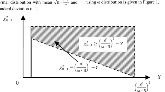
Where D is semi-width interval, d is a standardized value of the interval midpoint, and Y is a squared normal distributed with
mean · −
� and standard deviation of 1. Based on Equation (3), we can obtain the cumulative distribution function (CDF) of � using ω distribution. It is expressed in Equation (4).
� � � =� � � =�
3· 2−1+
� =�
�·3 2
− 2−1 (4)
Where � denotes � random variable and takes only positives values.
� � � =� 2−1
�·3 2
− = − +
2· · 2−1 −1 2 ·
−1 2 ·
∞
�·3 2
−
�·3 2
0
=1−0 �·32 − + 2· ·� −12 �·32− · (5)
Where (·) is the density function of a normal distribution with mean · −
� and standard deviation of 1.
Cumulative distribution function of Cpm
using ω distribution is given in Figure 1.
Figure 1. Cumulative distribution function of � using ω distribution
The estimated capability index, � is a random variable with � distribution. So, the cumulative distribution function of � can be used to calculate the control chart limits and efficiency of the control chart.
2.2 Estimation of Cpm using chi-square distribution
Using the representation in Equation 2, Cpm
can be rewrittenas below:
� = 2− 1
6 · 2+ ( − )2=
2− 1
6 · � ·
�2· 2+ ·
− �
2
To derive the probability density function and the cumulative distribution function of
Cpm the estimator of Cpm can be expressed
as:
� = 2−1
6·� · 2 �2+ · −�
2≡ 2−1
6·� 2, =
3 2,
(6)
Where χn,2 denotes a non-central Chi-Square distribution with n degrees of freedom and we get:
= · −
�
Where is the parameter of the non-central Chi-Square distribution.
3.
Control chart limits for
C
pmSpecifying the control limit is one of the critical decisions that must be made in designing a control chart. These control limits are chosen so that if the process is in control, all of the sample points will fall between them. As long as the points plot within the control limits, the process is assumed to be in control, and no action is necessary. However, a point that plots outside of the control limits is interpreted as evidence that the process is out of control, and investigation and corrective action is required to find and eliminate the assignable cause (Lin and Sheen, 2005; Maiko et al., 2009). Essentially, the control chart is a test of the hypothesis that the process is in a state
of statistical control. To determine if a given process meets the preset capability requirement, we can consider the statistical testing with null hypothesis H0 (Cpm = Cpm0)
and alternative hypothesis H1 (Cpm Cpm0).
For an initial study, we use the samples that are in control to calculate the value of Cpm0using the estimators =x for process
mean and � = / 2 for standard deviation.
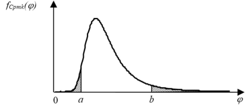
� � � = � 0 = 1− �
Where a denotes lower confidence limit and b denotes upper confidence limit, Cpm0
denotes Taguchi capability index when the process is in control.
Considering Equation (7), we obtain the distribution of Cpm given in Figure 2. The
distribution of � is constructed using Mathcad software.
Figure 2. Distribution of the estimated Cpm
3.1 Calculation of control limits using � distribution
Numerous methods for constructing approximate confidence interval have been proposed in the literature (Costa, 1998; Novoa and Noel, 2008). In this paper, the control graphic limits are computed using ω distribution and Chi-Square distribution. Firstly, the control limits using ω distribution is constructed. A 100 (1 - α) % confidence
interval estimation is shown in Equation (8).
� � � = � 0 = 1− � (8)
Using the distribution function of ω the control limits are computes as:
=�01-α 2and =�0α2
And upper and lower control limits of Cpm
� =�0� 2
� = � 0
� =�0 1−� 2
3.2 Calculation of control limits using Chi-Square distribution
We can also compute the control limits using Chi-Square distribution. Replacing the estimator of Cpm in the Chi-Square distribution, we can obtain a 100(1-α)% confidence interval estimation shown in Equation (9).
� 0
3 2, 0
= 1− � (9)
Hence, we get
� 3 0
1
, 0
2
3
0
= 1− �
By some simplifications:
� 02
9 2 , 0
2 0
2
9 2 = 1− �
Using the Chi-Square distribution, the control limits are computed as follows:
= 0
3· 2(, 0�/2)
and = 0
3· 2(1, 0−�/2)
And upper control limit and lower control limit can be expressed as:
� = 0
3 · ,
0 2(1−�/2)
� = � 0
� = 0
3· 2(, 0�/2)
3.3 Efficiency study on Cpm using ω distribution
The efficiency of control chart is determined by average run length. The speed with which a control chart detects process shift measures its statistical efficiency. An efficient chart balances the cost by operating out-of-control and the cost of maintaining the control chart. However, for fixed chart costs, the quicker and out-of-control state is detected, the better is the quality of a chart. The ability of control charts to detect shifts in process is described by their operating characteristic curves. The operating characteristics of � can be defined as:
� =� � � � �
Replacing the value of control limits defined in previous section, we have:
� =� �01−� 2 � �0� 2/ �
Where �0 is the value of � for 0and �0. Using cumulative distribution function, the operating characteristics take the form below:
� =� � �0� 2 − � � �01−� 2 (10)
3.4 Efficiency study on Cpm using Chi-square distribution
� =� � � � / � = � 0
3 · ,
0 2(�/2) �
0
3 · ,
0 2(1−�/2)
By some simplifications, we can construct the operating characteristics as below:
� = � 2− 1
6 ·�0
· ,
0 2(�/2)
2− 1
6 · σ · , 0 2(�/2)
2− 1
6 ·�0
· ,
0 2(1−�/2)
And we have:
� = �0
2
�2· , 0 2�2
, 2 �02
�2· , 0 21−�2
=
, 0 2(�/2)
� ,
2 , 0
2(1−�/2)
�
Where rv is the variance ratio.
Also, using the cumulative distribution function of � , the operating characteristics can be written as:
� ( � ) =�
,
2 , 0
2(�/2)
�
− � 2, , 0
2(1−�/2)
�
Where the probability density function of a non-central Chi-Square with n degree of freedom is given in Equation (12).
,
2 = −2 · �
�!·
2+�−1· −2
22+2�·� 2+� ∞
�=0 > 0 (12)
And the cumulative distribution function can be shown as below:
� 2, = −2· �
�!·
2+�−1· −2
22+2�·� 2+� ∞
�=0
0 · > 0 (13)
4.
Distribution of the Estimated
C
pmkThe index of Cpmk takes into account the
location of the process mean between two specification limits, the proximity to the target value, and the process variation. It has been shown to be a useful capability index for processes with two-sided specification limits. If the target value is centered in the tolerance interval midpoint (T=M), the Cpmk
index can be defined as:
� � = 3·� �(22+(− ,−−)12)
We know that:
� , =1
2· + − 1
2· −
� � = 2−1
2 −
2+1
2 − μ
3 · �2+ ( − )2=
− −
3 · �2+ ( − )2=
− −
3 · �2+ ( − )2
Using above Equation, we can express the estimator of Cpmk:
� � = − −
3· 2+( − )2 (14)
Changing some variables, � � distribution is written as:
� � = ~
− , � 2−
3�
· 2−1+n · N μ−T
σ ,
1 n
2 =
·
� −
−
� , 1
2
3 · 2−1+N μ−T
σ , 1
2
By some simplifications, we have:
� � = −
3· 2−1+
(15)
Based on Equation (15), we can obtain the
cumulative distribution function of � �using distribution, as expressed in Equation (16).
� � � =� � � =� −
3 · 2−1+ =�
−
3 · −1
2 +
� − 3· 2 2−1+ =� − 3· 2
− 2−1 (16)
Where denotes � �andom variable and takes only positives values.
Cumulative distribution function of � �
defined in Equation (16) is given in Figure 3.
Using Equation (16), we can compute the cumulative distribution function of � � as
below:
� � � =� 2 − 3·
2
− = − +
2· · 2−1 −1 2 ·
∞
− 3·
2
−
3· +1 2
0
−12· =1−0 3· +12 − + 2· ·� −12 − 3· 2− (17)
4.1 Control chart limits for Cpmk
To determine if a given process meets the preset capability requirement, we can consider the statistical testing with null hypothesis H0 (Cpmk = Cpmk0) and alternative
hypothesis H1 (Cpmk Cpmk0). In this study,
we search two control limits, namely a andb computed below:
� � � � � = � �0 = 1− �
Where Cpmk0 is Taguchi real capability index
when the process is in control.
Considering above Equation, we obtain the distribution of � �given in Figure 4. To construct the distribution of � � is conducted Mathcad software.
Figure 4.Distribution of the Estimated Cpmk
Using the distribution function of � �, the values of a andb are computed as:
= 01−� 2and = 0� 2
And the control limits for Cpmk can be expressed as below:
� � = 0
� 2
� � = � �0
� � = 0 1−� 2
Where UCLCpmk is the upper control limit of Cpmk, CLCpmk is the center line of Cpmk and LCLCpmk is the lower control limit of Cpmk.
4.2 Efficiency study on Cpmk
� =� � � � � � � � �
Using the value of control limits computed
in Section 4.1, the operating characteristic of � �
can be constructed as:
� =� 01−� 2 � � 0� 2 =� � � 0� 2 − � � � 01−� 2 (18)
Where 0 is the value of � � for 0 and �0.
5.
Efficiency comparison of the
capability control charts with
joint
�
and
R
charts
The purpose of the process monitoring is the detection of any assignable causes that changes µ from 0 to 1= 0+ �0 , where
≠0 and that changes σ from�0 to�1=
�0 , where ≠0. Varying the values of μ
and σ, we obtain the efficiency of capability
control charts and joint and R control charts. For a control chart, the detection speed of the process shifts shows its statistical performance. In this section, the performance of Cpm and Cpmk capability
control charts is compared with the performance of a traditional and R control charts. We use as sample size values of n=3 and n=5, that are the most usual. The Cpm
control chart has been obtained using the � distribution of the Cpm, and the Cpmk
controlchart has been obtained using the distribution of the Cpmk. The numerical
examples given in Costa’s paper (1998) are used to compare the results. The obtained results are displayed in Tables 1 and 2. Table 1 presents the efficiency values both capability-traditional control charts for sample size of 3.
As seen in Table 1, for given sample size of n, the performance of all the control charts increases as and increases. For small values of ( 1.75), the and R charts are better for detecting small shifts, but for
large values of ( 2), Cpm chart are
slightly better for detecting larger shifts. In other words, Cpm control chart catches the
shifts faster than the joint and R charts for
=3, and both of them have almost same performance for =2. When increases ( 0.5), for low values of (<1.5), Cpmk
control chart are better for detecting assignable causes than Cpmcontrol chart,
conversely, for high values of ( 1.5), the performance of the Cpm control chart is
better than Cpmk control chart. Table 2
summarizes the efficiency values for capability and traditional control charts for sample size of 5.
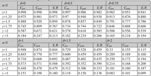
From Table 2, it is evident that when and increases the performance of all the charts increases (except for the values of and R charts, and Cpmk chart for = 2). Also, when
increases ( 0.5) for especially large values of ( 1.75), Cpm control chart is
the best for detecting assignable causes. For small values of ( 1.5), Cpmk control
chart catches the shifts faster than Cpm
control chart. After all, it is seen that, the results obtained for different sample size are similar.To compare the efficiency of Cpm and Cpmk control charts we provide the operating
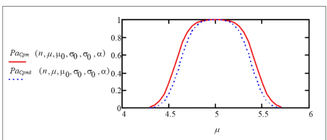
characteristics curves shown in Figure 5-8. For calculating the operating characteristics, we use the process parameters as T=5, T1=4, T2=6, 0=5, 0=0.2, n=5, 0.0024. Figure 5
presents the operating characteristic curves of Cpm and Cpmk control charts (standard
Table 1. The efficiency comparison of the control charts for n=3, with α=0.0024
n=3 =0 =0.5 =0.75
Cpm Cpmk �, Cpm Cpmk �, Cpm Cpmk �,
=1 0.998 0.998 0.998 0.995 0.991 0.990 0.988 0.976 0.973 =1.25 0.982 0.986 0.978 0.968 0.965 0.959 0.946 0.932 0.929 =1.5 0.930 0.95 0.923 0.904 0.916 0.896 0.871 0.872 0.859 =1.75 0.841 0.887 0.837 0.812 0.849 0.808 0.776 0.803 0.771 =2 0.735 0.804 0.735 0.708 0.769 0.708 0.676 0.727 0.676 =3 0.377 0.469 0.387 0.367 0.455 0.375 0.354 0.437 0.363
n=3 =1 =1.5 =2
Cpm Cpmk �, Cpm Cpmk �, Cpm Cpmk �,
=1 0.969 0.94 0.934 0.859 0.761 0.742 0.598 0.443 0.415 =1.25 0.907 0.876 0.876 0.763 0.687 0.690 0.530 0.425 0.425 =1.5 0.822 0.808 0.804 0.672 0.627 0.636 0.473 0.407 0.422 =1.75 0.726 0.740 0.719 0.590 0.576 0.576 0.424 0.39 0.405 =2 0.631 0.671 0.632 0.515 0.529 0.515 0.38 0.373 0.375 =3 0.337 0.414 0.346 0.291 0.353 0.301 0.238 0.283 0.248
Table 2. The Efficiency comparison of the control charts for n=5, with �=0.0024
n=5 =0 =0.5 =0.75
Cpm Cpmk �, Cpm Cpmk �, Cpm Cpmk �,
=1 0.998 0.998 0.998 0.997 0.986 0.982 0.982 0.953 0.941 =1.25 0.975 0.981 0.973 0.97 0.940 0.938 0.913 0.876 0.880 =1.5 0.888 0.920 0.894 0.878 0.857 0.849 0.791 0.777 0.786 =1.75 0.745 0.809 0.767 0.734 0.744 0.722 0.646 0.668 0.666 =2 0.587 0.672 0.621 0.578 0.618 0.585 0.506 0.556 0.539 =3 0.184 0.247 0.213 0.182 0.234 0.206 0.165 0.218 0.194
n=5 =1 =1.5 =2
Cpm Cpmk �, Cpm Cpmk �, Cpm Cpmk �,
Figure 5. Operating characteristic curves of Cpm and Cpmk control charts (σ=σ0)
We observe that Cpmk control chart has more
power than Cpm control chart to detect the
changes in the mean, assuming that standard deviation is constant. The operating
characteristic curves of Cpm andCpmk control
charts are shown in Figure 6 (σ=0.5, process mean changes).
Figure 6. Operating characteristic curves of Cpm and Cpmk control charts (σ=0.5)
As seen in Figure 6, for a small changes in the process mean, the efficiency of the Cpm
control chart is better than the Cpmk. Also, the
performance of Cpm and Cpmk are almost
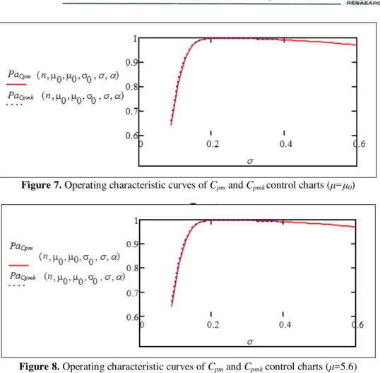
same for larger shifts in the process mean.Figure 7 provides the operating characteristic curves of Cpm and Cpmk control
charts (process mean is in control, standard deviation changes).
It is clear that both of the operating characteristic curves are very similar for all the values of the standard deviation. So, we ensure that, the performance of Cpm andCpmk
control charts is the same. Operating characteristics curves of Cpm and Cpmk
control charts are given in Figure 8 ( =5.6, process standard deviation changes). As seen in Figure 8, Cpmk control chart is more
effective than Cpm control chart. It is
concluded that, the performance of the Cpm
control chart seems better for detecting changes in the process mean. However, Cpmk
Figure 7. Operating characteristic curves of Cpm and Cpmk control charts ( = 0)
Figure 8. Operating characteristic curves of Cpm and Cpmk control charts ( =5.6)
6.
Application example: a
simulation study
We consider an example to illustrate the design procedure which is described in the previous section. In order to test the applicability of the proposed Cpm control
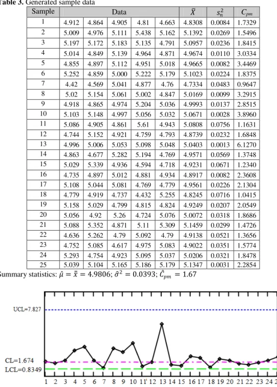
chart we conduct a simulation study. In this study, a random sample size of 5, for 25 subgroups was generated by simulation. The obtained results are displayed in Table 3.
Under the assumption that, these samples are taken from the normal distribution with mean 5 and standard deviation of 0.2. Using the distribution which is previously explained, we obtain the upper control limit UCL, is set to 7.827, the lower control limit, LCL, is set to 0.8349. The control chart of Cpm for the generated sample data is shown
Table 3. Generated sample data
Sample Data 2 C
pm 1 4.912 4.864 4.905 4.81 4.663 4.8308 0.0084 1.7329 2 5.009 4.976 5.111 5.438 5.162 5.1392 0.0269 1.5496 3 5.197 5.172 5.183 5.135 4.791 5.0957 0.0236 1.8415 4 5.014 4.849 5.139 4.964 4.871 4.9674 0.0110 3.0334 5 4.855 4.897 5.112 4.951 5.018 4.9665 0.0082 3.4469 6 5.252 4.859 5.000 5.222 5.179 5.1023 0.0224 1.8375 7 4.42 4.569 5.041 4.877 4.76 4.7334 0.0483 0.9647 8 5.02 5.154 5.061 5.002 4.847 5.0169 0.0099 3.2915 9 4.918 4.865 4.974 5.204 5.036 4.9993 0.0137 2.8515 10 5.103 5.148 4.997 5.056 5.032 5.0671 0.0028 3.8960 11 5.086 4.905 4.861 5.61 4.943 5.0808 0.0756 1.1631 12 4.744 5.152 4.921 4.759 4.793 4.8739 0.0232 1.6848 13 4.996 5.006 5.053 5.098 5.048 5.0403 0.0013 6.1270 14 4.863 4.677 5.282 5.194 4.769 4.9571 0.0569 1.3748 15 5.029 5.339 4.936 4.594 4.718 4.9231 0.0671 1.2340 16 4.735 4.897 5.012 4.881 4.934 4.8917 0.0082 2.3608 17 5.108 5.044 5.081 4.769 4.779 4.9561 0.0226 2.1304 18 4.779 4.919 4.737 4.432 5.255 4.8245 0.0716 1.0415 19 5.158 5.029 4.799 4.815 4.824 4.9249 0.0207 2.0549 20 5.056 4.92 5.26 4.724 5.076 5.0072 0.0318 1.8686 21 5.088 5.352 4.871 5.11 5.309 5.1459 0.0299 1.4726 22 4.636 5.262 4.79 5.092 4.79 4.9138 0.0521 1.3656 23 4.752 5.085 4.617 4.975 5.083 4.9022 0.0351 1.5774 24 5.293 4.754 4.923 5.095 5.037 5.0206 0.0321 1.8478 25 5.039 5.104 5.165 5.186 5.179 5.1347 0.0031 2.2854 Summary statistics: = = 4.9806; � 2= 0.0393;
� = 1.67
Figure 9. The Control chart of Cpm for the generated sample data
Using Cpm control chart, we conclude that
process seems to be capable for initial study.
We can recommend using Cpm for
specifications. It is seen that the proposed approach can be applied in a simple way. To control the process using the Cpmk control
chart, the procedure is similar. To derive Cpmk control chart same calculations can be
performed the over the same observations.
7.
Conclusions
Traditionally, and chart is used to control the process mean and aR chart is used to control the process variance. In this paper, we propose a new process capability control chart design for monitoring the process mean, standart deviation simultaneously.
Since capability control
chartssimultaneously measures process variability and centering they would provide a convenient way to monitor changes in process capability after statistical control is established. We have shown that it is possible to design one chart which can monitor the mean, variability and the
deviation from the specification limits at the same time.In this study, the efficiency of Cpm
and Cpmk capability control charts are
investigated. In addition, the efficiency of the proposed Cpm and Cpmk control charts is
compared with a joint and R control charts. It is seen that Cpm control chart is
more effective to detect the changes in the process mean. Nevertheless, Cpmk control
chart has more power to detect the changes in the process variance.It is demonstrated that how the new developed approach efficiently monitors capable but unstable processes by detecting the variation of the capability level. When the process shift is large the practitioners can use the suggested capability control chart design efficiently. The designed capability control charts are very useful in the case where one wants to compare the efficiency of the capability and traditional joint -R control charts, since, none of the techniques proposed in the literature, so far, can be used in such cases.
References:
Bordignon, S., & Scagliarini, M. (2006). Estimation of Cpmwhen measurement error is present. Quality and Reliability Engineering International. 22(7), 787–801.
Boyles, R.A. (1991). The Taguchi capability index. Journal of Quality Technology, 23(1), 17-26.
Chan, L.K., Cheng, S.W., & Spiring, F.A. (1988). A new measure of process capability: Cpm. Journal of Quality Technology, 29(3),162-165.
Chang, Y. C., & Wu, C.W. (2008). Assessing process capability based on the lower confidence Chen, G., Cheng, S.W., & Xie, H. (2001). Monitoring process mean and variability with one
EWMA chart. Journal of Quality Technology, 33, 223–233.
Chena, J., Zhubc, F., Lib, G.Y., Maa, Y.Z., & Tuc, Y.L. (2012). Capability index of a complex-product machining process. International Journal of Production Research, 50(12), 3382–3394.
Costa, A.F. (1998). Joint X and R charts with variable parameters. IIE Transactions. 30, 505-514.
Costa, A.F., & Rahim, M.A. (2004). Monitoring process mean and variability with one non-central Chi-Square chart. Journal of Applied Statistics, 31(10), 1171–1183.
Grau, D. (2011). Process yield and capability indices, Communications in Statistics—Theory and Methods, 40, 2751–2771.
Jeang, A. (2010). Optimal process capability analysis for process design. International Journal of Production Research. 48(4), 957–989
Jiao, Y.B., & Djurdjanovic, D. (2010). Joint allocation of measurement points and controllable tooling machines in multistage manufacturing processes. IIE Transactions, 42(10), 703–720. Kane, V.E. (1986). Process capability indices. Journal of Quality Technology. 18(1), 41-52. Lin, G.H. (2006). Evaluating process centering with large samples – an approximate lower
bound on the accuracy index. International Journal of Advanced Manufacturing Technology. 28, 149–153.
Lin, H.C., & Sheen, G.J. (2005). Practical implementation of the capability index Cpk based on the control chart data. Quality Engineering. 17, 371-390.
Mahesh, B.P., & Prabhuswamy, M.S. (2010). Process variability reduction through statistical process control for quality improvement. International Journal for Quality Research. 4(3), 193-203.
Maiko, M., Arizono, I., Nakase, I., & Takemoto, Y. (2009). Economical operation of the Cpm control chart for monitoring process capability index. International Journal of Advanced Manufacturing Technology. 43,304-311.
Novoa, C., & Noel, A.L. (2008). On the distribution of the usual estimator of Cpkand some applications in SPC. Quality Engineering, 21, 24-32.
Pearn, W.L. Kotz, S., & Johnson, N.L. (1992). Distributional and inferential properties of process capability indices. Journal of Quality Technology, 24(4), 216-231.
Pearn, W.L., & Lin, P.C. (2004). Testing process performance based on capability indices Cpk with critical values. Computers and Industrial Engineering, 47, 351-369.
Pearn, W.L., & Shu, M.H. (2003). Lower confidence bounds with sample size information for Cpmapplied to production yield assurance. International Journal of Production Research. 41(15), 581-3599.
Pearn, W.L., Shu, M.H., & Hsu, B.M. (2005). Testing process capability based on Cpm in the presence of random measurement errors. Journal of Applied Statistics, 32(10), 1003-1024. Perakis, M.(2010). Estimation of differences between process capability indices Cpm or Cpmk
for two processes. Journal of Statistical Computations and Simulation. 80(3),315-334. Tai, Y.T. (2011). Evaluating process capability under undetected fluctuations. IEEE Int’1
Technology Management Conference. 484-487.
Wu, C.W., Pearn, W.L., & Kotz, S. (2009). An overview of theory and practice on process capability indices for quality assurance. International Journal Production Economics. 117, 338-359.
Appendix: Symbols used in the calculus:
n - sample size - samplemean
sn - sample standard deviation
0 - mean value when the process is in control
σ0 - standard deviation when the process is in control 1- mean value when the process is out of control
T1 - lower specification limit T2 - upper specification limit M - tolerance interval midpoint D - semi-width interval
- parameter of the non-central Chi-Square distribution - standardized value of the interval midpoint
Cpm - Taguchi capability index
Cpm0 - Taguchi capability index whenwhen the process in control Cpmk - Taguchi real capability index
Cpmk0 - Taguchi real capability indexwhen the process in control rv - the variance ratio
ω - Cpm random variable
φ - Cpmk random variable UCL - upper control limit CL - central control line LCL - lower control limit
María Teresa Carot
University of Valencia Polytechnic,
Departament of Statistics Operation Research and Applied Quality Valencia Spain
Aysun Sagbas
University of Namik Kemal
Department of Industrial Engineering,
Tekirdag Turkey
José María Sanz
University of Valencia Polytechnic,