Global modelling of direct and indirect effects of sea spray aerosol using a source function encapsulating wave state

(1)

ACPD

14, 4537–4597, 2014

Direct and indirect e_ffects of sea spray

aerosol

A.-I. Partanen et al.

Title Page

Abstract Introduction

Conclusions References

Tables Figures

◭ ◮

Back Close

Full Screen / Esc

Printer-friendly Version

Interactive Discussion

Discussion

P

a

per

|

D

iscussion

P

a

per

|

Discussion

P

a

per

|

Discuss

ion

P

a

per

|

Atmos. Chem. Phys. Discuss., 14, 4537–4597, 2014 www.atmos-chem-phys-discuss.net/14/4537/2014/ doi:10.5194/acpd-14-4537-2014

Atmospheric Chemistry and Physics

Open Access

Discussions

This discussion paper is/has been under review for the journal Atmospheric Chemistry and Physics (ACP). Please refer to the corresponding final paper in ACP if available.

Global modelling of direct and indirect

e

_ff

ects of sea spray aerosol using

a source function encapsulating wave

state

A.-I. Partanen1, E. M. Dunne1, T. Bergman1, A. Laakso1, H. Kokkola1, J. Ovadnevaite2, L. Sogacheva3, D. Baisnée4, J. Sciare4, A. Manders5, C. O’Dowd2, G. de Leeuw3,6, and H. Korhonen1

1

Atmospheric Research Centre of Eastern Finland, Finnish Meteorological Institute, Kuopio, Finland

2

School of Physics and Centre for Climate and Air Pollution Studies, Ryan Institute, National University of Ireland Galway, University Road, Galway, Ireland

3

Climate change, Finnish Meteorological Institute, Helsinki, Finland

4

LSCE, CEA-CNRS-UVSQ, Laboratoire des Sciences du Climat et de l’Environnement, Gif-sur-Yvette, France

5

TNO, Utrecht, the Netherlands

6

(2)

ACPD

14, 4537–4597, 2014

aerosol

Title Page

Tables Figures

◭ ◮

Back Close

Full Screen / Esc

Discussion

P

a

per

|

D

iscussion

P

a

per

|

Discussion

P

a

per

|

Discuss

ion

P

a

per

|

Received: 23 December 2013 – Accepted: 11 February 2014 – Published: 20 February 2014

Correspondence to: A.-I. Partanen (antti-ilari.partanen@fmi.fi)

(3)

ACPD

14, 4537–4597, 2014

aerosol

Title Page

Tables Figures

◭ ◮

Back Close

Full Screen / Esc

Discussion

P

a

per

|

D

iscussion

P

a

per

|

Discussion

P

a

per

|

Discuss

ion

P

a

per

|

Abstract

Recently developed parameterizations for the sea spray aerosol source flux, encapsu-lating wave state, and its organic fraction were incorporated into the aerosol-climate model ECHAM-HAMMOZ to investigate the direct and indirect radiative e_ffects of sea spray aerosol particles. Our simulated global sea salt emission of 805 Tg yr−1

(uncer-5

tainty range 378–1233 Tg yr−1) was much lower than typically found in previous stud-ies. Modelled sea salt and sodium ion concentrations agreed relatively well with mea-surements in the smaller size ranges at Mace Head (annual normalized mean model bias₋13 % for particles with vacuum aerodynamic diameterD_va<1 µm), Point Reyes (₋29 % for particles with aerodynamic diameter Da<2.5 µm) and Amsterdam Island

10

(₋52 % for particles withD_a<1 µm) but the larger sizes were overestimated (899 % for particles with 2.5 µm < D_a<10 µm) in Amsterdam Island. This suggests that at least the high end of the previous estimates of sea spray mass emissions is unrealistic. On the other hand, the model clearly underestimated the observed concentrations of or-ganic or total carbonaceous aerosol at Mace Head (₋82 %) and Amsterdam Island

15

(₋68 %). The large overestimation (212 %) of organic matter at Point Reyes was due to the contribution of continental sources. At the remote Amsterdam Island site, the organic concentration was underestimated especially in the biologically active months, suggesting a need to improve the parameterization of the organic sea spray fraction. Globally, the satellite-retrieved AOD over the oceans, using PARASOL data, was

un-20

derestimated by the model (means over ocean 0.16 and 0.10, respectively); however, in the pristine region around Amsterdam Island the measured AOD fell well within the simulated uncertainty range. The simulated sea spray aerosol contribution to the in-direct radiative effect was positive (0.3 W m−2), in contrast to previous studies. This positive effect was ascribed to the tendency of sea salt aerosol to suppress both the

25

(4)

ACPD

14, 4537–4597, 2014

aerosol

Title Page

Tables Figures

◭ ◮

Back Close

Full Screen / Esc

Discussion

P

a

per

|

D

iscussion

P

a

per

|

Discussion

P

a

per

|

Discuss

ion

P

a

per

|

to a strong negative direct effect, the simulated effective radiative forcing (total radia-tive) e_ffect was₋0.2 W m−2_{. The simulated radiative e}

ffects of the primary marine or-ganic emissions were small, with a direct effect of 0.03 W m−2and an indirect effect of −0.07 W m−2.

1 Introduction

5

The magnitude of the aerosol radiative effect remains a large unknown in current es-timates of anthropogenic effects on radiative forcing (Forster et al., 2007). One of the key quantities needed for better estimates of anthropogenic radiative forcing is an ac-curate estimate of the radiative effects from natural aerosol (Carslaw et al., 2013). It is, after all, the change from the natural background that is important when

quantify-10

ing human e_ffects on the climate. With over 71 % of the Earth’s surface covered by oceans, sea spray aerosol makes a significant contribution to the Earth’s radiation bal-ance (Haywood et al., 1999; Rap et al., 2013). Because of their high global emissions and relatively large sizes, sea spray aerosol particles provide a major contribution to the scattering of solar radiation (cf. de Leeuw et al., 2011), and to a lesser extent of thermal

15

radiation (Li et al., 2008). Furthermore, their size and hygroscopicity make them effi -cient cloud condensation nuclei (CCN) and they can therefore a_ffect the Earth’s climate by modifying marine cloud properties and lifetime (Pierce and Adams, 2006; Korhonen et al., 2008).

The current estimates of global sea spray aerosol emissions remain highly uncertain

20

(de Leeuw et al., 2011), and values ranging over several orders of magnitude have been presented based on recent modelling studies (Textor et al., 2006; Gantt et al., 2012; Grythe et al., 2013). Much of this variation is due to uncertainties in the wind speed dependence of the production flux, or the upper cut-o_ff size of the sea spray aerosol particles included in the models, but also to different experimental methods

25

(5)

ACPD

14, 4537–4597, 2014

aerosol

Title Page

Tables Figures

◭ ◮

Back Close

Full Screen / Esc

Discussion

P

a

per

|

D

iscussion

P

a

per

|

Discussion

P

a

per

|

Discuss

ion

P

a

per

|

spray aerosol particles as a function of particle size, location and time remains poorly quantified (Albert et al., 2012; Gantt and Meskhidze, 2013). While inorganic compo-nents constitute most of the global sea spray aerosol mass, during biologically active months organic compounds contribute significantly to, and can in some cases even dominate, the mass of submicron sea spray aerosol particles (Novakov et al., 1997;

5

O’Dowd et al., 2004; Facchini et al., 2008; Sciare et al., 2009; Fuentes et al., 2010a, b; King et al., 2012). Recent measurements have indicated that the organic fraction con-sists of a myriad of chemically distinct types of surface-active compounds (Hawkins and Russell, 2010; Schmitt-Kopplin et al., 2012), but the exact identity of these com-pounds is largely unknown. Uncertainties also remain regarding the mixing state of

10

the organic matter with sea salt (Middlebrook et al., 1998; Leck and Bigg, 2005; Hultin et al., 2010). Furthermore, Ovadnevaite et al. (2011) noticed that sea spray particles enriched in organic matter show a dichotomous behaviour in terms of water uptake, in that they have a low hygroscopicity in subsaturated conditions but act as very e_fficient cloud condensation nuclei (CCN) in supersaturated conditions. All these unknowns and

15

poorly constrained phenomena lead to the current large uncertainty in our estimates of sea spray aerosol radiative e_ffects (Gantt and Meskhidze, 2013).

Recently, Ovadnevaite et al. (2014) developed a new sea spray aerosol source func-tion by combining measurements of aerosol number concentrafunc-tion at the Mace Head station (O’Connor et al., 2008) and open-ocean eddy correlation fluxes during the

SEA-20

SAW cruise (Norris et al., 2012). Instead of the commonly used 10 m wind speed, this source function parameterizes the particle production as a function of the Reynolds number and thus encapsulates the influences of wave height and history as well as sea water viscosity (dependent on the sea surface temperature and salinity). While the new source function predicts sea spray aerosol fluxes on the lower end of other

25

(6)

ACPD

14, 4537–4597, 2014

aerosol

Title Page

Tables Figures

◭ ◮

Back Close

Full Screen / Esc

Discussion

P

a

per

|

D

iscussion

P

a

per

|

Discussion

P

a

per

|

Discuss

ion

P

a

per

|

This study provides a further evaluation of the Ovadnevaite et al. (2014) sea spray aerosol source function against a variety of in situ and remote sensing measure-ments. We have implemented the source function into the global aerosol-climate model ECHAM-HAMMOZ, and extended the parameterization to include organic enrichment of sea spray aerosol particles based on recent work by Rinaldi et al. (2013). After the

5

evaluation, we use the source function together with ECHAM-HAMMOZ to provide es-timates of the direct and indirect radiative effects of sea spray aerosol and the impact of organic enrichment of sea spray aerosol particles to radiative e_ffects.

2 Methods

2.1 Climate model ECHAM-HAMMOZ

10

The global aerosol-climate model ECHAM-HAMMOZ (ECHAM5.5-HAM-SALSA) (Stier et al., 2005; Zhang et al., 2012; Bergman et al., 2012) consists of an atmospheric core model ECHAM, which solves the fundamental equations for atmospheric flow and physics, and tracer transport, and of an aerosol model HAM. In this study, aerosol microphysics was calculated using the sectional model SALSA (Kokkola et al., 2008;

15

Bergman et al., 2012). SALSA describes the aerosol population consisting of sulphate, sea salt, organic matter, black carbon and dust using 10 size sections to cover the size range from 3 nm to 10 µm, with 10 additional sections to account for the external mixing of particles. The model resolves the aerosol processes of nucleation of new particles (Kulmala et al., 2006), condensation of sulphuric acid and organic gases onto

20

pre-existing particles, coagulation, hydration, and removal of particles via dry and wet deposition.

The anthropogenic and biomass burning aerosol emissions in the model were taken from AeroCom-II ACCMIP data (Riahi et al., 2007, 2011). Natural emissions were sim-ulated as described in Zhang et al. (2012), apart from the sea salt and primary marine

25

(7)

be-ACPD

14, 4537–4597, 2014

aerosol

Title Page

Tables Figures

◭ ◮

Back Close

Full Screen / Esc

Discussion

P

a

per

|

D

iscussion

P

a

per

|

Discussion

P

a

per

|

Discuss

ion

P

a

per

|

tween aerosols and radiation were calculated online (Zhang et al., 2012), and the total aerosol direct e_ffect was diagnosed by a second call of the radiation routine without any aerosols. The first and second indirect effects were calculated following Lohmann and Hoose (2009). The activation of aerosol particles into cloud droplets was calculated with the physically based parameterization of Abdul-Razzak and Ghan (2002).

5

2.2 Implementation of the sea spray aerosol source function

The standard version of ECHAM-HAMMOZ simulates the sea salt source flux by com-bining the parameterizations of Gong et al. (2003) with dry diameter between 50 and 400 nm, of Monahan et al. (1986) for particles with dry diameter between 400 nm and 8 µm, and of Andreas (1998) for particles with dry diameters of and 8–10 µm (Guelle

10

et al., 2001; Bergman et al., 2012). Furthermore, it does not include emissions of PMOM. For the current study, we implemented the recently developed source func-tion by Ovadnevaite et al. (2014) into the model, and combined it with the approach of Rinaldi et al. (2013) to account for the fraction of PMOM as a function of chlorophylla concentration and 10 m wind speed.

15

The Ovadnevaite et al. (2014) parameterization describes the sea spray aerosol flux in the size range 15 nm–6 µm in diameter, whereas the aerosol module SALSA used in this study tracks sea spray aerosol particles between 30 nm and 10 µm. Corre-spondingly, we used the Ovadnevaite parameterization for the particle diameter range 30 nm–6 µm, and extended it over the size range 6–10 µm by using (the shape of) the

20

Monahan (1986) source function, but matching the flux at 6 µm with the Ovadnevaite et al. (2014) flux. Using this approach, the simulated sea spray aerosol flux for particles larger than 6 µm was significantly lower than in the original Monahan (1986) formula-tion. Hereafter, we refer to the original parameterization by Ovadnevaite et al. (2014) as the OSSA source function, and to the combined flux parameterization of Ovadnevaite

25

(8)

ACPD

14, 4537–4597, 2014

aerosol

Title Page

Tables Figures

◭ ◮

Back Close

Full Screen / Esc

Discussion

P

a

per

|

D

iscussion

P

a

per

|

Discussion

P

a

per

|

Discuss

ion

P

a

per

|

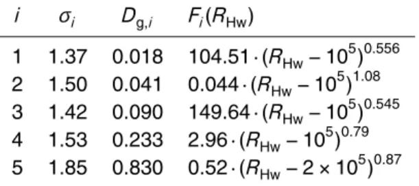
The Ovadnevaite et al. (2014) sea spray aerosol source function has been parame-terized in terms of five lognormal modes (Table 1):

dF d log₁₀D =

5 X

i=1

F_i(R_Hw) √

2πlog₁₀σ_i exp 

  −

1 2



 

log₁₀_DD

g,i

log₁₀(σi) 

 

2

  

, (1)

whereD is particle dry diameter, σ_i and D_g,i, are geometric standard deviation and geometric mean (count-median) dry diameter of mode i, respectively, and Fi(RHw) is

5

total number flux of modei depending on the Reynolds number

R_Hw=u_∗H_s/ν_w. (2)

Hereu_∗is the friction velocity calculated online by the ECHAM-HAMMOZ model,Hsis the significant height of wind-generated waves taken from 6 hourly ECMWF reanalysis data (see Sect. 2.3), andν_w is the temperature-dependent kinematic viscosity of sea

10

water. We calculated the viscosity by linear interpolation from the values in Table 2 and by assuming that the salinity of sea water is 35 g kg−1 _{(see Ovadnevaite et al. (2014)}

for a discussion on the effect of salinity).

Number and volume fluxes of sea spray aerosol particles for each of the SALSA size sections below 6 µm were calculated by integrating over each of the five modal

15

OSSA emissions distributions separately. For particles smaller than 700 nm in diam-eter, SALSA tracks both number and mass separately. In the size range 30–700 nm, both the number and volume distributions were integrated for each section. In the size range above 700 nm, the size sections in SALSA have a fixed dry diameter and only the aerosol number is tracked in each section. It was therefore not possible to set both

20

(9)

ACPD

14, 4537–4597, 2014

aerosol

Title Page

Tables Figures

◭ ◮

Back Close

Full Screen / Esc

Discussion

P

a

per

|

D

iscussion

P

a

per

|

Discussion

P

a

per

|

Discuss

ion

P

a

per

|

Due to the nature of its derivation, using data obtained in the winter with low biological activity, the OSSA source function represents the total emission of sea spray aerosol particles. In this work, due to lack of further information, it was assumed that the total emission flux does not change during periods of higher biological activity – that is, the function describes the total flux, including both sea salt and PMOM. For sea spray

5

aerosol particles larger than 700 nm in diameter, SALSA does not explicitly track the organic fraction, i.e. all sea spray aerosol particles are assumed to consist solely of sea salt. This introduces a relatively small error since these large particles contain only a small fraction of organic matter (Facchini et al., 2008). For smaller particles, the mass fraction of the PMOM in the sea spray aerosol emissions (f_PMOM) was calculated

10

following Rinaldi et al. (2013):

f_PMOM=(0.569_×c_Chl_a)+(₋0.0464_×u_{10 m}+0.409), (3)

wherec_Chla is the chlorophyll a concentration in surface water (µg m−3) and u10 m is the 10 m wind speed (m s−1). The chlorophyllaconcentration in the current study was taken from GlobColour satellite retrievals (http://www.globcolour.info), as it was in

Ri-15

naldi et al. (2013). We used the mean value of the previous eight-day period to account for the lag in correlation between organic mass fraction and chlorophyllaconcentration (Rinaldi et al., 2013) (see Sect. 2.3 for details).

To distinguish PMOM from organics from other sources, the aerosol model was ex-tended to include a new tracer for PMOM in each of the four size sections in the range

20

30–700 nm. The density of the PMOM was assumed to be 1300 kg m−3, its molar mass was set to 150 g mol−1_{, and its refractive index was set to 1.48}

×10−9i at all wave-lengths to reflect recent measurements (Aas, 1996; Kanakidou et al., 2005; Nessler et al., 2005; Vaishya et al., 2013)

As mentioned earlier, Ovadnevaite et al. (2011) observed that PMOM at Mace Head

25

(10)

ACPD

14, 4537–4597, 2014

aerosol

Title Page

Tables Figures

◭ ◮

Back Close

Full Screen / Esc

Discussion

P

a

per

|

D

iscussion

P

a

per

|

Discussion

P

a

per

|

Discuss

ion

P

a

per

|

salt and PMOM was calculated from

LWC_SS₊_PMOM=(V_SS+V_PMOM)_×(HGF3₋1)_×ρ_w, (4)

where V_SS and V_MOC are the volume concentrations of sea salt and marine PMOM and ρ_w is the density of water. The hygroscopic growth factor HGF was obtained by bi-linear interpolation of the values from the look-up table by Vaishya et al. (2013)

5

for the relative humidity and PMOM mass fraction in each model grid box. The total LWC of the particles was calculated by adding up LWC_SS₊_MOC and LWC for other aerosol compounds calculated using the ZSR method (Stokes and Robinson, 1966) as described in Kokkola et al. (2008).

Since a theoretical understanding of the high CCN activity of PMOM is currently

lack-10

ing, we tuned the modelled cloud activation of PMOM to approximately match the ob-servations of Ovadnevaite et al. (2011). In order to do this, we used the cloud-activation subroutine of the model (Abdul-Razzak and Ghan, 2002) in a 0-dimensional framework together with a representative marine aerosol size distribution from the model simula-tions. We then adjusted the dissociation coe_fficient of PMOM (i.e. how many ions each

15

PMOM molecule dissociates into in a solution) within this subroutine so that when the mass fraction of PMOM was 50 %, all soluble particles larger than 30 nm in diame-ter were activated at a supersaturation of about 0.7 % (cf. Ovadnevaite et al., 2011). The best match was obtained when the dissociation coefficient was set to five. It is important to note that the chosen value of dissociation coe_fficient a_ffects only the cloud

20

activation routine of the model and is not physically based. Its purpose is only to fit the model results to match observations of Ovadnevaite et al. (2011).

2.3 Input data for the sea spray aerosol source function

ECHAM-HAMMOZ is an atmosphere-only model and therefore does not predict the significant height of wind-generated ocean waves. However, this quantity was needed

25

(11)

ACPD

14, 4537–4597, 2014

aerosol

Title Page

Tables Figures

◭ ◮

Back Close

Full Screen / Esc

Discussion

P

a

per

|

D

iscussion

P

a

per

|

Discussion

P

a

per

|

Discuss

ion

P

a

per

|

Centre for Medium-range Weather Forecasts (ECMWF) at a 6 h time resolution over the whole simulated time period (Uppala et al., 2005). Since all model simulations presented in this study were nudged to the ECMWF winds, the off-line wave height data is expected to correspond well to the simulated surface wind fields.

The 1◦

×1◦ wave height data from the Global Wave Analysis Data Set was

interpo-5

lated to the ECHAM-HAMMOZ model resolution of T63. Since the land–sea masks of the wave height data and the ECHAM-HAMMOZ model were not identical, we needed to fill in some blank values over the model ocean grid cells after the interpolation. This was done by using the average values of the neighbouring grid cells in the blank grid cells.

10

The chlorophyll a data needed to calculate the PMOM mass fraction of sea spray aerosol emissions (Eq. 3) was obtained from GlobColour satellite retrievals. Glob-Colour provides two chlorophyll retrievals, CHL1 and CHL2. The CHL1 data set makes use of the assumption that variations in ocean colour in open water are attributed to phytoplankton or co-varying substances, and the retrieval algorithms make use of this

15

assumption. Near the coast, other dissolved substances can cause significant changes in ocean colour, and the retrieval algorithms used to provide the CHL2 data set try to take account of this.

We used eight-day-mean 1◦_×1◦ GlobColour retrievals of CHL1 and CHL2 data for the years 2005–2010. The data sets were combined by using the CHL2 data within

20

4 grid boxes of the coast and the CHL1 data elsewhere (Garver–Siegel–Maritorena (GSM) model; Maritorena and Siegel, 2005). Due to cloud cover and breaks in satellite observations, there were still large gaps present in the data set. These gaps were filled using the Multiple Singular-Spectrum Analysis (MSSA) toolkit Spectra (Kondrashov and Ghil, 2006). MSSA works by fitting periodic functions to the data. The maximum

25

(12)

ACPD

14, 4537–4597, 2014

aerosol

Title Page

Tables Figures

◭ ◮

Back Close

Full Screen / Esc

Discussion

P

a

per

|

D

iscussion

P

a

per

|

Discussion

P

a

per

|

Discuss

ion

P

a

per

|

A large portion of the winter hemisphere is outside the satellite field of view. This systematic omission of winter-time data is a major challenge in providing a chlorophyll data set suitable for use in a global climate model, as the fitting algorithms will not cap-ture the low winter-time chlorophyll values when only provided with high summer-time data. To remedy this, we first read in the maximum and minimum observed latitude from

5

each eight-day-mean satellite retrieval file. Outside of this latitude range, the chlorophyll concentration in a given grid cell (C_i) was then set according to the following formula:

Ci =Cb×

1 2

lati−latb 4

, (5)

whereC_bis the value in the nearest marine grid cell to the latitude boundary, lat_i is the latitude (in degrees) of grid celli, and lat_bis the latitude of the boundary value (either

10

highest or lowest latitude with a value for chlorophyll concentration). Due to the extreme seasonal variations in chlorophyll at high latitudes, this method may still lead to some underestimation in the summer hemisphere, where polar chlorophyll values can be extremely high, and some overestimation in the winter hemisphere where chlorophyll would be close to zero (cf. Albert et al., 2012, for a discussion of the effect of gap-filling

15

methods). However, it is still expected to provide more accurate values than simply filling in winter-time values based on summer observations.

After the temporal gap-filling was done for the chlorophylladata, the remaining gaps, due to either totally missing data in some grid-cells or di_fferences in land–sea masks between the data and our model, were filled with the same procedure as described

20

above for the wave height data.

2.4 Observational data for model evaluation

2.4.1 In-situ measurements to evaluate aerosol chemical composition

(13)

ACPD

14, 4537–4597, 2014

aerosol

Title Page

Tables Figures

◭ ◮

Back Close

Full Screen / Esc

Discussion

P

a

per

|

D

iscussion

P

a

per

|

Discussion

P

a

per

|

Discuss

ion

P

a

per

|

the west coast of Ireland (O’Connor et al., 2008). Aerosol measurements are per-formed by sampling ambient particles at 10 m a.g.l. through a community air-sampling duct. The size-resolved non-refractory chemical composition of submicron aerosol par-ticles is measured with an Aerodyne High Resolution Time of Flight Aerosol Mass Spectrometer (ToF-AMS) deployed in standard mode (DeCarlo et al., 2006).

HR-5

ToF-AMS particulate matter with (vacuum aerodynamic) diameter below 1 µm (PM₁) sea salt concentrations were derived following the method described in (Ovadnevaite et al., 2012). The HR-ToF-AMS was routinely calibrated according to the methods de-scribed by Jimenez et al. (2003) and Allan et al. (2003). The measurements were performed with a time resolution of 5 min and a vaporizer temperature of _∼650◦C.

10

Composition-dependent collection e_fficiency was applied for the measurements used here, and ranged from 0.45 to 0.97. Aerosol size distributions and number concen-trations were measured using a scanning mobility particle sizer (SMPS) system. The system comprised of a di_fferential mobility analyzer (DMA, TSI model 3071), a conden-sation particle counter (TSI model 3010), and an aerosol neutralizer (TSI 3077). The

15

aerosol diameter range covered was 3–500 nm. Before their sizes were measured, the particles were dried to a relative humidity below 40 %. For this study. we used the Mace Head measurement data covering both marine and continental air masses to make the results comparable with modelled mean conditions.

Continuous physico-chemical measurements of marine aerosol are undertaken also

20

at Amsterdam Island atmospheric research station (37◦₄₈′_{S, 77}◦₃₄′_{E, see Fig. 1),}

located in the southern Indian Ocean sector of the Austral Ocean. The station is located at 3400 km and 5000 km from the nearest upwind lands (Madagascar and South Africa, respectively). Throughout most of the year, it benefits from pristine ma-rine conditions, especially during the summer when high-pressure conditions and low

25

(14)

ACPD

14, 4537–4597, 2014

aerosol

Title Page

Tables Figures

◭ ◮

Back Close

Full Screen / Esc

Discussion

P

a

per

|

D

iscussion

P

a

per

|

Discussion

P

a

per

|

Discuss

ion

P

a

per

|

(gravimetry) and ion composition analyses, and on pre-fired quartz filters for EC and OC measurements. Aerosol size segregation was achieved using a four-stage cascade impactor (Dekati Ltd) running at 30_±1 LPM. A detailed description of the site charac-teristics and the chemical analytical protocols used to determined ions and carbon con-tents in aerosols is provided by Sciare et al. (2009). Given the remote character of the

5

site, no clean-sector strategy was necessary to avoid local contaminations. However, a post-sampling data treatment was applied to the database, discarding all samples as-sociated with an equivalent black carbon (EBC) value higher than 10 ng C m−3_{, which}

effectively excludes all anthropogenically contaminated samples. To compare the mea-surements with the modelled total carbonaceous aerosol mass concentrations, the total

10

carbon concentration measurements from Amsterdam Island were multiplied with 1.8 to account for compounds other than carbon.

Chemical aerosol composition data from Point Reyes (Fig. 1) were obtained from the Interagency Monitoring of Protected Visual Environments (IMPROVE) network. PM_2.5 sulphate, sea salt and organic matter concentrations were deployed in this study. Ion

15

chromatography methods from the Nylasorb substrate, extracted ultrasonically in de-ionized water, are used by the IMPROVE network to analyse inorganic ions, while organic carbon is analysed from quartz fiber filters. An average ambient particulate or-ganic compound was assumed to have a constant fraction of carbon by weight (56 %), which was used to correct the organic carbon mass for other elements (in addition to

20

carbon) associated with the assumed organic molecular composition. Therefore, or-ganic matter (OM) mass concentration is assumed to be OM=1.8_·OC where OC is organic carbon mass concentration. A detailed IMPROVE monitoring program descrip-tion is presented by Malm et al. (2004).

Simulated sea spray aerosol mass concentration values in Europe were evaluated

25

(15)

ACPD

14, 4537–4597, 2014

aerosol

Title Page

Tables Figures

◭ ◮

Back Close

Full Screen / Esc

Discussion

P

a

per

|

D

iscussion

P

a

per

|

Discussion

P

a

per

|

Discuss

ion

P

a

per

|

and the Na+/SS ratio is therefore 22.99/58.44. We have compared monthly mean values from both the model and the observations. In cases where a single model grid box contained more than one station, we averaged the stations’ data. Aerodynamic diameter was used for the cut-o_ffdiameter of PM_2.5and PM₁₀ in the model.

2.4.2 Satellite and sun-photometer data for aerosol optical depth comparison

5

For the evaluation of the modelled aerosol optical depth (AOD), i.e. the column-integrated extinction, two independent data sets were used: AERONET sun photome-ter data and satellite retrieved AOD. AERONET is a global network of sun photomephotome-ters (Holben et al., 1998) which directly measure the solar radiation as well as scattered (dif-fuse) radiation over a large number of angles. Together this information provides highly

10

accurate information on the aerosol properties at each site. The AOD is measured with an accuracy of 0.015 (Eck et al., 1999). In our study we used monthly-mean cloud-screened and quality assured Level 2.0 data from 17 island and 24 coastal AERONET stations which have at least one month of data in the period 2006–2010, and which are located below 2000 m altitude. The 500 nm AERONET AOD measurements were

15

interpolated to 550 nm using τ₅₅₀=τ₅₀₀_×(550/500)−α_{, where} _τ

500 and τ550 are the AODs for 500 nm and 550 nm, respectively. Forα, we use the monthly mean Ångström exponent for extinction between 440 nm and 870 nm (Mielonen et al., 2011).

The second data source used was the AOD retrieved from the POLDER (Polariza-tion and direc(Polariza-tionality of the Earth’s Reflectances) radiometer onboard the PARASOL

20

(Polarization and Anisotropy of Reflectances for Atmospheric Science coupled with Observations from a Lidar) satellite. Launched in year 2005 as part of the A-train mis-sion (L’Ecuyer and Jiang, 2010), PARASOL has a sun-synchronized orbit with 1.30 p.m. ascending node.

The POLDER instrument measures the polarized light in di_fferent directions and at

25

(16)

ACPD

14, 4537–4597, 2014

aerosol

Title Page

Tables Figures

◭ ◮

Back Close

Full Screen / Esc

Discussion

P

a

per

|

D

iscussion

P

a

per

|

Discussion

P

a

per

|

Discuss

ion

P

a

per

|

using PARASOL data with AERONET ground-based measurements (Holben et al., 1998) has shown a very good correlation (0.91) with a bias of around 0.03 (Breon et al., 2010). Validation of the PARASOL AOD using different statistical methods has shown that PARASOL provides a very high accuracy over ocean and covers features well (de Leeuw et al., 2014).

5

Aerosol products retrieved with PARASOL (Tanre et al., 2011) are provided at an 18.5 km_×18.5 km resolution. For the comparison with model results, PARASOL AOD for the oceans was remapped to the model resolution of T63 and interpolated into wavelength of 550 nm using monthly-mean Ångström exponent from PARASOL.

2.5 Design of the experiments

10

To test the new source function we set up several model simulations, summarized in Table 3. The control simulation (control) had no sea spray aerosol emissions at all. Our baseline run (ossa-ref) simulated the sea spray aerosol flux using the extended OSSA source function, as described in Sect. 2.2. In order to separate the respective radiative e_ffects of sea salt and PMOM, we also made a run using the extended OSSA source

15

function, but excluding PMOM emissions (simulationossa-salt).

Ovadnevaite et al. (2014) estimated that the uncertainty in the submicron part of their source function is in the range of 55–60 %. It is caused by uncertainties in e.g. particle concentration measurements and boundary layer height. Therefore, to test the sensitivity of our results to these uncertainties, we set up two sensitivity runs (

ossa-20

lowfluxandossa-highflux) in which the sea spray aerosol flux from the extended OSSA

source function was multiplied by 0.4 and 1.6, respectively.

When comparing the simulated aerosol fields with in situ and remote sensing mea-surements, discrepancies may arise, not only from uncertainties in the modelled source function, but also from uncertainties in the modelled removal mechanisms. To test

25

(17)

ACPD

14, 4537–4597, 2014

aerosol

Title Page

Tables Figures

◭ ◮

Back Close

Full Screen / Esc

Discussion

P

a

per

|

D

iscussion

P

a

per

|

Discussion

P

a

per

|

Discuss

ion

P

a

per

|

(ossa-ref). In-cloud scavenging coefficient gives the fraction of in-cloud aerosol

par-ticles inside cloud droplets. In case of precipitation, they are removed from the at-mosphere. The low and high values of in-cloud scavenging coefficients for the size ranges of 30–70 nm and 700 nm–10 µm were estimated using measurements by Hen-ning et al. (2004). They measured the scavenging coe_fficients for liquid phase clouds

5

to be about 1 at the diameter of about 400 nm, and hence we used 0.99 for the larger size range also in the simulationossa-low-ics. In-cloud scavenging is a major removal mechanism for marine aerosol (Textor et al., 2006) and the modelled aerosol burdens have been shown to be sensitive to in-cloud scavenging parameterizations in ECHAM-HAMMOZ (Croft et al., 2010).

10

For comparison, we also run the ECHAM-HAMMOZ model with its default sea spray aerosol source function (see Sect. 2.2), i.e. using a combination of Gong et al. (2003), Monahan et al. (1986), and Andreas (1998) source functions without any PMOM emis-sions (simulationdefault-salt).

All simulations were run with a model resolution T63L31, corresponding to a 1.9◦

×

15

1.9◦grid in the horizontal and 31 vertical levels extending to 10 hPa. The model meteo-rology was nudged towards the reference state of the ERA-interim reanalysis data (Dee et al., 2011). Sea surface temperatures were prescribed from the reanalysis data. The model runs covered the years 2006–2010 and were preceded with a five-year spin-up to allow the aerosol system to reach equilibrium. The first four years and ten months

20

of the spin-up had no sea spray aerosol emissions. Each simulation then had a final two-months spin-up period using the appropriate sea spray aerosol emissions.

3 Evaluation of the extended OSSA source function

3.1 Emissions and burdens

Table 5 summarizes the emissions and burdens of sea salt and PMOM in the di_ff

er-25

(18)

ACPD

14, 4537–4597, 2014

aerosol

Title Page

Tables Figures

◭ ◮

Back Close

Full Screen / Esc

Discussion

P

a

per

|

D

iscussion

P

a

per

|

Discussion

P

a

per

|

Discuss

ion

P

a

per

|

805 Tg yr−1_{in the PM}

10size range, with the sensitivity simulations using the extended OSSA source function suggesting a range of 378–1233 Tg yr−1. These values were ap-proximately an order of magnitude lower than the 7229 Tg yr−1 _{yielded by the default}

ECHAM-HAMMOZ sea-spray aerosol source function in the default-salt simulation, and on the low side of previously reported estimates. The AeroCom phase I models

5

simulated a median global sea salt emission of 6280 Tg yr−1 _{(mean 16 600 Tg yr}−1₎

(Textor et al., 2006). More recently, Tsigaridis et al. (2013) compared several different sea spray aerosol source functions within their global model and obtained a range of global sea salt emissions from 2272 to 12 462 Tg yr−1_{. Grythe et al. (2013) reviewed 21}

different sea salt source functions and calculated annual mean emissions in the range

10

of_∼1830–2.44_×106Tg yr−1. On the other hand, the simulations by Gantt et al. (2012) provided a global sea salt emission of 73.6 Tg yr−1_{, which is clearly lower than values}

obtained in this study. These data demonstrate the large uncertainties associated with current estimates of sea spray aerosol emissions. (Note that only a fraction of the dis-crepancy is explained by di_fferent model studies using di_fferent upper cut-o_ffsizes for

15

the sea salt emissions).

The simulated sea salt burden in the current study was also at the low end of pub-lished values, consistent with the low emissions obtained using the OSSA source func-tion (Ovadnevaite et al., 2014). The baseline runossa-ref gave a burden of 2.9 Tg, and the sensitivity simulations a range of 1.2–4.6 Tg. Of the sea salt burden, 17 % was in

20

the size range of PM₁, 42 % in PM_1–2.5, and 41 % in PM_2.5–10. Again, these values were approximately an order of magnitude lower than those obtained using the default sea spray aerosol flux in ECHAM-HAMMOZ (12.9 Tg in simulation default-salt) and also smaller than the AeroCom phase I median burden of 6.37 Tg (mean 7.52 Tg) (Textor et al., 2006). It is interesting to note that the uncertainty due to the in-cloud scavenging

25

in stratiform clouds had a negligible effect on the simulated sea salt burden (runs

ossa-low-icsandossa-high-ics). However, this is in line with a sensitivity study by Andersson

(19)

ACPD

14, 4537–4597, 2014

aerosol

Title Page

Tables Figures

◭ ◮

Back Close

Full Screen / Esc

Discussion

P

a

per

|

D

iscussion

P

a

per

|

Discussion

P

a

per

|

Discuss

ion

P

a

per

|

was evaluated. In their study, they found that the aerosol size distributions were fairly insensitive to in-cloud scavenging parameters when using SALSA.

Our baseline simulation predicted global PMOM emissions of 1.1 Tg yr−1(sensitivity range 0.5–1.8 Tg yr−1; see Table 5). This value was well in the range of 0.1–11.9 Tg yr−1 simulated by Gantt et al. (2012), who compared six di_fferent ways to estimate the

or-5

ganic mass fraction of sea spray aerosol emissions. It should be noted, however, that the simulated PMOM emissions are sensitive to the choice of sea spray aerosol source function, and that the sea salt emissions predicted in Gantt et al. (2012) are even lower than the ones obtained in this study. The estimated magnitude of submicron PMOM emissions in other previous studies were typically much higher than we simulated here,

10

in the range of 2.8–76 Tg yr−1_{(Gantt et al., 2011; Vignati et al., 2010; Mezkhidze et al.,}

2011; Tsigaridis et al., 2013).

While one reason for the relatively low PMOM emissions in the current study was the extended OSSA source function, which gave sea spray aerosol emissions in the lower end of the published range, it should be noted that most of the previously published

es-15

timates have assumed that the organic mass fraction in the emitted sea spray aerosol is determined solely by the chlorophyll a concentration. Gantt et al. (2011) showed, however, that there is a clear inverse correlation between the organic mass fraction and the wind speed, as high winds result in mixing of the organic-enriched surface layer with below-surface waters. The parameterization used in this study (Eq. 3) takes

20

this e_ffect into account through the use of the Rinaldi et al. (2013) parameterization, leading to low organic fractions in high-wind-speed regions even when the chlorophylla concentration is high (_∼1 mg m−3_{) (Fig. 2). Regionally, the reduction of the organic}

frac-tion with increasing wind speed was most evident in the Southern Ocean, where wind speeds are high (on average about 10 m s−1) but the organic fraction was mostly

be-25

(20)

ACPD

14, 4537–4597, 2014

aerosol

Title Page

Tables Figures

◭ ◮

Back Close

Full Screen / Esc

Discussion

P

a

per

|

D

iscussion

P

a

per

|

Discussion

P

a

per

|

Discuss

ion

P

a

per

|

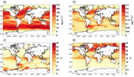
As expected, the largest sea salt emissions were seen in southern mid-latitudes (Figs. 3a and 4a) where the surface-level wind speeds are consistently high throughout the year. Another region with high sea salt emissions was the northern mid-latitudes (Fig. 3a), especially in the winter months (Fig. 4a). However, the emissions in this region showed large seasonal variation. Across these latitude bands, the sea salt fluxes

5

were typically lowest in the summer months (Fig. 4a). This implies that the seasonal changes in wind speed are much more important than seasonal changes in sea surface temperature in terms of determining the total sea spray aerosol flux.

Despite the small organic fraction in emitted sea spray aerosol in the southern mid-latitudes, some of the highest marine PMOM emissions in terms of mass were seen in

10

this region (Figs. 3b and 4c). This was due to the very high total sea spray aerosol emis-sions in these high wind speed regimes. Another prominent source region of PMOM was the Northern Hemisphere mid-latitudes, where emissions were especially high in the autumn months (Fig. 4c). Comparing Fig. 4a and c, it is evident that the seasonality and zonal patterns of sea salt and PMOM di_ffered quite a lot. PMOM showed a strong

15

seasonal variation due to the seasonality of biological activity, especially polewards of ±50◦ latitude, while the seasonal variation of the sea salt emissions was largest in the mid-latitudes and Southern Hemisphere tropics. Furthermore, whereas the contribution of low latitudes to global sea salt emissions was small, a significant fraction of PMOM was emitted from these regions, especially in the boreal summer months.

20

It is also worth noting that the simulated sea spray aerosol emissions (Fig. 4a and c) and burdens (Fig. 4b and d) showed very di_fferent zonal behaviour. For example, while the emissions of both sea salt and PMOM were relatively low at low latitudes compared to the mid-latitudes, the burdens of both compounds peaked in the tropics due to sig-nificantly slower removal in that region and possibly transport of sea spray from the

25

(21)

ACPD

14, 4537–4597, 2014

aerosol

Title Page

Tables Figures

◭ ◮

Back Close

Full Screen / Esc

Discussion

P

a

per

|

D

iscussion

P

a

per

|

Discussion

P

a

per

|

Discuss

ion

P

a

per

|

3.2 Comparison to in-situ measurements

We compared the simulated aerosol mass concentrations and size distributions ob-tained using the extended OSSA source function with the high-quality long-term obser-vations available from one marine (Amsterdam Island) and two coastal (Mace Head, Point Reyes) sites as described in Sect. 2.4 and Fig. 1.

5

The Mace Head station on the west coast of Ireland makes measurements of the PM₁ concentrations of sulphate, sea salt and organic matter, and of the aerosol size distribution. The cut-o_ffsize of 1 µm in the PM₁measurements was based on vacuum aerodynamic diameter, i.e.D_va=0.8_·D_·(ρ/1000), whereDis modelled particle diam-eter andρ is particle density. Since the grid-cell containing the exact location of the

10

Mace Head station is defined as “land” in the model, and thus included continental emissions but not sea spray aerosol emissions, we used the adjacent grid-cell to the west of the site in our comparison with in situ measurements. This grid-cell is defined as “sea” in the model and showed about 40 % higher sea salt concentrations compared to the grid-cell containing the exact Mace Head location.

15

Figure 5 shows the monthly-mean sulphate, sea salt, and total organic matter (both continental and PMOM) PM₁ concentrations in Mace Head for the years 2009 and 2010. The sea salt concentration at this site was captured well by the model with both the extended OSSA source function and the default sea salt source function in ECHAM-HAMMOZ (simulationsossa-ref anddefault-salt, respectively): the measured sea salt

20

concentration fell within the simulated uncertainty range of the extended OSSA source function (defined by the sensitivity simulationsossa-highflux,ossa-lowflux, ossa-high-ics, andossa-low-ics) in 19 out of 22 months with measurement data available. How-ever, on average the simulationossa-ref tended to underestimate sea salt concentra-tions slightly (normalized mean bias of₋13 %).

25

(22)

ACPD

14, 4537–4597, 2014

aerosol

Title Page

Tables Figures

◭ ◮

Back Close

Full Screen / Esc

Discussion

P

a

per

|

D

iscussion

P

a

per

|

Discussion

P

a

per

|

Discuss

ion

P

a

per

|

predicting the seasonal variation of sulphate, the same was not true for organic matter. Note that both the measured and the simulated sulphate and organic matter concentra-tions shown in Fig. 5 also include material emitted from continental sources (only 15 % of modelled organic matter was PMOM on two-year average at Mace Head). There-fore, some of the poor match between the model and observations is likely to have

5

arisen from uncertainties in continental emissions. Even in the summer time, when the organic fraction of sea spray aerosol peaks according to the measurements (e.g., O’Dowd et al., 2004), 80 % of the modelled organic matter concentration originated from continental sources. Therefore, it seems likely that the parameterization used in the study for predicting the organic fraction of the sea spray aerosol (Rinaldi et al.,

10

2013) is unable to capture all the nuances of PMOM emissions.

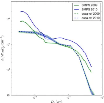
Figure 6 shows the observed (solid lines) and modelled (dashed lines) annual mean size distributions at Mace Head for years the 2009 and 2010. The model captured the size distribution reasonably well between 20–200 nm, but underestimated the size dis-tribution below 20 nm and above 200 nm. The underestimation of the nucleation mode

15

was expected, since the model included only activation nucleation of sulphuric acid (Kulmala et al., 2006) while previous observations from Mace Head have suggested that iodine nucleation is likely to play an important role at this site (O’Dowd et al., 2002). The underestimation of the large accumulation mode particles was likely caused mostly by the poor model skill in simulating the aerosol organic matter content (cf. Fig. 5c),

al-20

though uncertainties in simulating the sulphate and sea salt aerosol sources may also have contributed to some extent.

Figure 7 depicts the modelled mass concentrations at Amsterdam Island together with measurements of sodium ion (Na+) mass concentration in three size classes (PM₁, PM_1–2.5, and PM_2.5–10), and total carbonaceous aerosol concentration for PM₁ (using

25

(23)

ACPD

14, 4537–4597, 2014

aerosol

Title Page

Tables Figures

◭ ◮

Back Close

Full Screen / Esc

Discussion

P

a

per

|

D

iscussion

P

a

per

|

Discussion

P

a

per

|

Discuss

ion

P

a

per

|

sea salt source function (simulationdefault-salt) in all three size ranges. In the largest size range, PM_2.5–10, the normalized mean bias was reduced from 4519 % in default-salt to 899 % in ossa-ref. As at Mace Head, the model underestimated (normalized mean bias of₋68 %) the total carbonaceous aerosol concentration (Fig. 7d). The un-derestimation was largest during the summer months, when the contribution of PMOM

5

is expected to be largest. The total carbonaceous aerosol concentration in the model consisted of 72 % continental organic matter, only 21 % PMOM, and 8 % black carbon. In the summer time, the modelled monthly-mean fraction of PMOM of total carbona-ceous aerosol peaked at 59 %. The fraction of PMOM was significantly less than was predicted by, e.g., Vignati et al. (2010), who calculated that the average primary

ma-10

rine fraction of organic carbon in the Southern Ocean in January and July would be more than 90 % and 80 %, respectively. The large relative contribution of continental emissions to total carbonaceous aerosol in our study was caused by the low emissions of PMOM, not high continental contribution in absolute terms as total carbonaceous aerosol was underestimated.

15

Figure 8 shows the observed and modelled PM_2.5(in terms of aerodynamic diame-ter) mass concentrations of sulphate, sea salt, and total (both continental and PMOM) organic matter for the years 2006–2010 at Point Reyes, which is located on the west coast of the US. Unlike Mace Head, the location of Point Reyes is defined as “sea” in the model, so we used the grid-cell containing Point Reyes for comparisons. The

20

model run with the extended OSSA source function captured the monthly mean values of observed sea salt concentrations well, with 70 % of the observed monthly mean val-ues falling within the modelled uncertainty range (Fig. 8b). The extended OSSA source function showed also a clear improvement over the default-salt run, with the normal-ized mean bias reduced from 50 % to ₋29 %. The sulphate mass concentration and

25

(24)

ACPD

14, 4537–4597, 2014

aerosol

Title Page

Tables Figures

◭ ◮

Back Close

Full Screen / Esc

Discussion

P

a

per

|

D

iscussion

P

a

per

|

Discussion

P

a

per

|

Discuss

ion

P

a

per

|

Reyes (monthly-mean fraction of PMOM of total organic matter was between 0.3–8 %). Thus, the overestimation of organic matter was caused by continental sources.

Figure 9 shows a comparison between simulated (ossa-ref) and observed (EMEP) monthly mean values of sodium ion concentration in PM_2.5and PM₁₀. Figure 9a shows a clear underestimation of the largest observed PM_2.5 monthly mean values. There

5

were no clear seasonal differences present in the observed values, but simulated win-ter values were larger than summer values. There was an even stronger seasonal dependence in PM₁₀in the model (Fig. 9b). Measured and modelled PM₁₀values also correlated better during the summer months, but in the winter the model clearly over-estimated the sodium ion concentration.

10

It is di_fficult to compare simulated values with point measurements, as the model cannot capture the subgrid-scale variability in aerosol concentrations. All except one of the measurement stations are located in grid boxes classified as “land”, meaning that there were no sea spray aerosol emission sources within the stations’ grid boxes. Some measurement stations are located quite near the coast, but stations which are further

15

inland can better represent modelled conditions as sea salt concentration gradients (and thus the sensitivity to grid-cell selection) were highest near the coasts.

3.3 Comparison to AOD measurements

The modelled AOD values (at wavelength of 550 nm) over the oceans were compared with satellite-retrieved AOD field (Fig. 10a). It has previously been shown that the

20

ECHAM-HAMMOZ-SALSA using the default sea spray aerosol source function (corre-sponding to our simulationdefault-salt) tends to overestimate the oceanic AOD derived from MODIS/MISR in the tropics and to underestimate at high latitudes (Bergman et al., 2012). This can be seen also in Fig. 10c, which shows the annual normalized mean bias between AOD calculated in the default-salt simulation and AOD retrieved from

25

(25)

ACPD

14, 4537–4597, 2014

aerosol

Title Page

Tables Figures

◭ ◮

Back Close

Full Screen / Esc

Discussion

P

a

per

|

D

iscussion

P

a

per

|

Discussion

P

a

per

|

Discuss

ion

P

a

per

|

When the default source function was replaced by the extended OSSA source func-tion (simulafunc-tion ossa-ref), the satellite-retrieved AOD was underestimated over most oceanic regions (Fig. 10b). As a result, the normalized mean bias over the oceans was −31 %. While the absolute value of the normalized mean bias to PARASOL was clearly smaller when using the default sea spray aerosol source function (13 %, Fig. 10c) than

5

the extended OSSA source function (₋31 %, Fig. 10b), this was mainly due to the large compensating over- and underestimations in different parts of the world when using the default source function. Normalized mean errors forossa-ref anddefault-saltwere 35 % and 41 %, respectively, showing that overall, the extended OSSA source func-tion improved the results. The extended OSSA source funcfunc-tion significantly improved

10

the agreement between model and measurements in the tropics and mid-latitudes, al-though it deteriorated somewhat at high latitudes (where satellite observations have the least coverage). The PARASOL values fell within the uncertainty range from

ossa-higflux and ossa-lowflux across 36 % of the ocean’s area (shaded area in Fig. 10b).

The model performed especially well in marine regions from the Equator to 45◦_{S, which} 15

represent some of the least polluted oceanic regions in the world, and are therefore dominated by natural aerosol emissions.

We made a more detailed evaluation of the model-predicted AOD against PARASOL data over the Southern Ocean (30–60◦S) and in proximity to the three stations dis-cussed in Sect. 3.2 (see the ocean masks used in Fig. 1). Over the Southern Ocean,

20

the extended OSSA source function tended to underestimate the satellite-retrieved AOD even when the uncertainty range is accounted for (Fig. 11a, compare black line with red line and shading). It is also apparent that the seasonal cycle in AOD was shifted compared to the measurements: whereas the peak monthly mean values were observed in the spring months, the model predicted the highest values in the middle

25

(26)

ACPD

14, 4537–4597, 2014

aerosol

Title Page

Tables Figures

◭ ◮

Back Close

Full Screen / Esc

Discussion

P

a

per

|

D

iscussion

P

a

per

|

Discussion

P

a

per

|

Discuss

ion

P

a

per

|

Around Amsterdam Island, the model captured the magnitude and also much of the seasonal variability of the observed AOD (Fig. 11b). The measured monthly AOD fell within the simulated uncertainty range (red shading) for all but six months (out of 60). However, there was a slight decreasing trend in the measured AOD which the model was unable to reproduce; as a result, the agreement between the baseline simulation

5

ossa-ref and the measurement improved towards the end of the simulated period. Part

of the good match between the modelled and measured AOD in this region is probably explained by underestimation of small particles and overestimation of large particles (Fig. 7) compensating the error of each other. Over this region, the model predicted that 69 % of the AOD is from sea spray aerosol (the difference between the solid red

10

and dashed black lines relative to the solid red line in Fig. 11b). The default sea spray aerosol source function in ECHAM-HAMMOZ (default-salt) predicted almost twice the observed AOD values (solid blue line).

Around Mace Head and Point Reyes, both of which are much more heavily influenced by continental emissions than Amsterdam Island, the modelled AOD values in the

ossa-15

ref run were clearly lower than the measured ones (Fig. 11b and c, respectively). At both sites, the model captured some features of the observed seasonal variation but underestimated most of the monthly peak values in winter/early spring by over 50 % or by absolute AOD value 0.1. It is worth noting that at both of these sites, the default-salt run gave a much better match with the measurements thanossa-ref. However, our

20

comparison with in situ mass concentrations (Fig. 5) suggests that the underestimation of AOD inossa-ref at Mace Head may be due to poor model performance in predicting the PMOM rather than the sea salt emissions.

We also compared the modelled monthly mean AOD to AERONET measurements (500 nm interpolated to 550 nm) at 17 island and 24 coastal stations (Fig. 12). The

25

(27)

sea-ACPD

14, 4537–4597, 2014

aerosol

Title Page

Tables Figures

◭ ◮

Back Close

Full Screen / Esc

Discussion

P

a

per

|

D

iscussion

P

a

per

|

Discussion

P

a

per

|

Discuss

ion

P

a

per

|

sons were 8.83 % (44.49 %),₋28.96 % (39.61 %),₋23.97 % (40.07 %), and₋11.98 % (36.50 %) for boreal winter, spring, summer, and autumn months, respectively.

4 Radiative e_ffects of sea spray aerosol particles

The radiative effects of sea spray aerosol particles were estimated from the difference between all-sky top-of-atmosphere net total radiation in each of the sea-spray

simu-5

lations and in thecontrol run. This method yields an effective radiative forcing (ERF) (also known as radiative flux perturbation) which includes both direct and indirect ef-fects (Haywood et al., 2009). The all-sky direct radiative e_ffect (direct component of ERF) of sea spray aerosol particles was calculated as follows: first, the radiation rou-tine during each time step was called with and without aerosol. The difference in total

10

net radiation between these calls was taken as the total (including all aerosols) aerosol direct effect of a given model run. Then, the direct radiative effect of sea spray aerosol particles was calculated from the difference in total aerosol direct effect between a sea-spray simulation and thecontrol run. The total indirect e_ffect (indirect component of ERF) of sea spray aerosol particles was calculated by subtracting the direct radiative

15

effect from the ERF (semi-direct effect of sea spray aerosol is negligible due to low absorption).

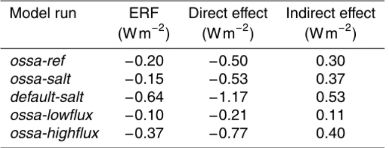
Table 6 summarizes the simulated global mean radiative effects of sea spray aerosol particles in the different runs. All our simulations predicted a negative ERF due to sea spray aerosol particles (i.e. total cooling e_ffect); however, the runs using the extended

20

OSSA source function showed much lower values (₋0.20 W m−2 in the baseline run

ossa-ref, with a sensitivity range from ₋0.10 to ₋0.37 W m−2) than the run using the

default sea spray aerosol source function in ECHAM-HAMMOZ (₋0.64 W m−2_in

simu-lationdefault-salt). Furthermore, our baseline simulationossa-ref gave a direct all-sky radiative effect of₋0.50 W m−2(sensitivity range from₋0.21 to₋0.77 W m−2) (Table 6).

25