The effect of hygroscopicity on eddy covariance estimates of sea-spray aerosol fluxes: a comparison of high-rate and bulk correction methods

(1)

www.atmos-meas-tech.net/6/323/2013/ doi:10.5194/amt-6-323-2013

Atmospheric

Measurement

Techniques

Geoscientiic

The effect of hygroscopicity on eddy covariance estimates of

sea-spray aerosol fluxes: a comparison of high-rate and bulk

correction methods

D. A. J. Sproson, I. M. Brooks, and S. J. Norris

Institute for Climate Atmospheric Science, School of Earth Environment, University of Leeds, UK

Correspondence to:D. A. J. Sproson (d.sproson@see.leeds.ac.uk)

Received: 14 August 2012 – Published in Atmos. Meas. Tech. Discuss.: 3 September 2012 Revised: 28 November 2012 – Accepted: 22 December 2012 – Published: 13 February 2013

Abstract.The eddy covariance technique is the most direct

of the methods that have been used to measure the flux of sea-spray aerosol between the ocean and atmosphere, but has been applied in only a handful of studies. However, unless the aerosol is dried before the eddy covariance measurements are made, the hygroscopic nature of sea-spray may combine with a relative humidity flux to result in a bias in the calculated aerosol flux. “Bulk” methods have been presented to account for this bias, however, they rely on assumptions of the shape of the aerosol spectra which may not be valid for near-surface measurements of sea-spray.

Here we describe a method of correcting aerosol spec-tra for relative humidity induced size variations at the high frequency (10 Hz) measurement timescale, where counting statistics are poor and the spectral shape cannot be well rep-resented by a simple power law. Such a correction allows the effects of hygroscopicity and relative humidity flux on the aerosol flux to be explicitly evaluated and compared to the bulk corrections, both in their original form and once reformulated to better represent the measured mean aerosol spectra. In general, the bulk corrections – particularly when reformulated for the measured mean aerosol spectra – per-form relatively well, producing flux corrections of the right sign and approximate magnitude. However, there are times when the bulk methods either significantly over- or underes-timate the required flux correction. We conclude that, where possible, relative humidity corrections should be made at the measurement frequency.

1 Introduction

Sea-spray aerosol, generated in the open ocean through bub-ble bursting in whitecaps, or as droplets are physically ripped from the crests of waves by the wind, is the second largest natural source of aerosol into the atmosphere after dust (Hop-pel et al., 2002). As such, sea spray is expected to have a major impact on global climate, both through direct (Doss-Hammel et al., 2002) and indirect effects (Haywood et al., 1999). An understanding of production rates and transport of sea-spray is, thus, a prerequisite for an understanding of the climate system as a whole. Sea-spray is also a poten-tially important mediator of air-sea fluxes of heat, moisture and momentum at high wind speeds (>25 m s−1) (Andreas, 1992), where large volumes of re-entrant sea-spray may be produced.

(2)

– again empirically – be related to the wind speed and sea-state, allowing a wind dependent sea-spray source function to be derived (Monahan et al., 1982, 1986). Other methods used to calculate the surface source function, albeit less fre-quently, include the gradient method (Petelski and Piskozub, 2006); inverse modelling (Vignati et al., 2001; de Leeuw et al., 2003) and concentration increase with fetch (Reid et al., 2001).

Although the equilibrium and whitecap methods discussed above have both been widely used, they are both indirect, and source functions spanning up to 6 orders of magnitude have been reported (Andreas, 1998, 2002). More recent stud-ies show source functions agreeing to within approximately one order of magnitude for particles with radii smaller than around 1 µm (de Leeuw et al., 2011), although the equilib-rium method is strictly only applicable to particles larger than about 3 µm (Petelski and Piskozub, 2006; Andreas et al., 2010). A more direct method to measure the sea-spray source function is through the eddy covariance technique, whereby turbulent fluctuations in the vertical component of the wind are correlated with fluctuations in the aerosol spectrum to produce a net vertical transport of aerosol particles (Nilsson et al., 2001; Geever et al., 2005; de Leeuw et al., 2007; Nor-ris et al., 2008, 2012). The derivation of a sea-spray source function using the eddy covariance method still, however, re-lies on some assumptions. Most importantly, what the eddy covariance technique actually measures is the net turbulent aerosol flux, therefore, it is only an adequate approximation to the true sea-spray source flux in conditions far from equi-librium. Note that this assumption is in direct contradiction of the conditions for which the equilibrium method is appli-cable, which relies on the assumption of zero net flux. In the limiting conditions of no deposition, or deposition equal to production, the eddy covariance or equilibrium method re-spectively give the best estimate of the surface source flux. However, neither of these methods can account for processes that occur below the measurement height, such as gas-to-particle conversion or coagulation of gas-to-particles. In practice, however, where deposition generally is non-zero, but smaller than production, both methods will result in an underestima-tion of the true surface source flux. It is also possible for deposition to exceed the surface source, in which case the equilibrium method will overestimate the source flux and the measured net eddy covariance flux will be of the wrong sign. In either case, eddy covariance measurement of the net flux corrected for deposition is the most direct method to deter-mine the surface source flux.

The calculation of an eddy covariance sea-spray source function requires the collocation of high-frequency aerosol and vertical wind measurements. This requires the use of a small, weatherproof aerosol spectrometer or a long sample line from the point of measurement back to the aerosol in-strument. The use of such a sample line introduces a num-ber of issues: a lag between wind and aerosol measurements; a damping of the aerosol fluctuations at high frequencies

and a loss of particles to the walls of the sample line. Cor-rections for these effects exist, but may rely on unproven assumptions or become significant for larger particle sizes

(r >1 µm). Using a compact in situ instrument with a short

sample line, however, makes drying the aerosol prior to mea-surement extremely difficult, thus, aerosol spectra will gen-erally be recorded at ambient humidity.

Sea-spray aerosol is extremely hygroscopic and particles will rapidly grow or shrink in response to changes in the lo-cal relative humidity. In the presence of an upward relative humidity flux (which is almost ubiquitous in the marine en-vironment), upward moving parcels of air (w′>0, wherew

is the vertical velocity and the prime indicates a perturba-tion from the mean) will, on average, have a higher relative humidity than downward moving parcels. As sea-spray re-sponds rapidly to RH fluctuations, a particle in an upward moving parcel may be larger than that in a downward mov-ing parcel, even when these particles have equal dry radius. When measuring these aerosol in discrete size bins, this ef-fect may cause the segregation of particles of equal dry radius into different bins, depending on the sign ofw′. When using the eddy covariance technique to determine aerosol flux, this will be interpreted as a net flux of aerosol, even if none exists. Fairall (1984), hereafter F84, and Kowalski (2001), hereafter K01, have both presented “bulk” methods of correcting for this apparent flux, based on mean meteorological conditions and assumptions of the shape of aerosol spectra within the marine boundary layer. Here, we describe a method of ac-counting for the humidity flux at the measurement timescale (a frequency of 10 Hz) and compare this to the bulk correc-tions of both F84 and K01 for measurements from the SEA-SAW cruise in North Atlantic during March–April 2007. In the next section, we discuss the theory behind the bulk cor-rection methods and describe the high-rate method we have used to account for humidity variance in the SEASAW data, give a brief overview of the SEASAW cruise, and processing that the data has undergone. In Sect. 3, we evaluate the va-lidity of the assumptions of spectral shape with regard to the SEASAW data and present some alternative functional forms which better represent the aerosol spectra for these data. In Sects. 4 and 5, we compare the biases calculated through the high-rate method with those from the bulk methods, both in their original forms, and having been reformulated to use the functional forms which better represent the mean spectra recorded during SEASAW.

2 Theory

(3)

number of deliquescent particles in a certain particle size in-terval is a non-conservative scalar and, thus, size-segregated eddy correlation measurements of the number flux, N′_w′_, whereN is the ambient aerosol concentration, may not be representative of the true aerosol flux, and net particle fluxes can be measured even where none are present.

2.1 Bulk corrections

Both F84 and K01 address the issue of apparent parti-cle fluxes, both through an apparent transfer velocity,1vd,

which is the transfer/deposition velocity induced through the vertical flux of saturation ratio. Both give the dependence of aerosol radius on humidity as

r(S)=r0

1+ γ

1−S 1₃

, (1)

wherer0is the dry aerosol radius andγis a parameter related

to the aerosol chemistry, taken as unity by F84 for clean ma-rine air. Taking the derivative of Eq. (1) with respect toS, we have

∂r

∂S =

γ r

3 1−S2

+3γ 1−S. (2)

Note: we have substitutedr0=r1+γ / 1−S

−1/3

in the above.

Under a fluctuation in saturation ratio,S′_{, the change in the} ambient concentration at a fixed radius is a combination of the translation of the particle distribution in radial space and a “renormalisation” which occurs due to the change in the size intervals over which the distribution is defined. These two effects result in an induced change in the particle distribution which can be written, following K01, as

N′=r′

" ∂N

∂r +

N r

#

. (3)

Both K01 and F84 make the assumption that the aerosol spectrum can be approximated through a Junge power law (Junge, 1963) of the form

N=αr−(β+1),

whereβis typically about 3 and, thus

N′

N = −β

r′

r. (4)

Combining Eqs. (2) and (4) with the definition of the deposi-tion velocity and taking ∂r

∂S ≡ r′

S′, we arrive at K01’s expres-sion for the bias velocity due to humidity fluctuations and hygroscopicity:

1vd=

−γ β

3(1−S)2₊₃_{γ (}₁₋_S)w

′_S′_. ₍₅₎

K01 reformulates Eq. (5) in terms of temperature and mois-ture fluxes, however, this is not required here. F84 makes the further approximation that, in the surface layer,

w′_S′₌_c

1 2

du∗(1−S), (6)

resulting in F84’s expression for the bias velocity:

1vd=

γ β

3 1+γ−Sc 1 2

du∗. (7)

Here,cdis the drag coefficient which can be calculated from

turbulence data or approximated through empirical relation-ships (Large and Pond, 1981; Yelland et al., 1998) andu∗is the friction velocity.

Both of these methods provide a bulk means of estimating the bias velocity due to hygroscopicity, but both rely on the assumption that aerosol spectra can be well represented with the use of a Junge power law, and F84’s equation relies on the accuracy of the approximation ofw′_S′_.

2.2 High-rate corrections

The collocation of high frequency measurements of humid-ity and size-resolved aerosol spectra during SEASAW allows the effect of hygroscopicity to be explicitly calculated. In or-der to do this, the 10 Hz CLASP spectra must be individually corrected to a reference humidity, typically the run-mean rel-ative humidity, following Zhang et al. (2006) and Lewis and Schwartz (2003).

Such a correction is relatively simple in the mean sense, where a long averaging period means that all size channels will have adequate counting statistics and a simple func-tional form (for example, a Junge power law) can be fitted to the mean spectrum. Under a humidity correction, chan-nel boundaries will change, but the number of particles,N, in each channel will be unchanged. Using the new channel boundaries, dN/dr and a new mean radius for each chan-nel can easily be calculated. If the spectrum is required over specific channel boundaries or at a specific radius, this can easily achieved by using the fit to the adjusted spectrum as an interpolant.

(4)

of the form dN_i₌airbi is then calculated for each channel in the adjusted spectrum, based on the values of dN/dr in that channel and those in any neighbouring channels. This fit provides an estimate of the particle distribution across each channel, as the significant gradient in concentration with size applies within as well as between channels, and needs ac-counting for in the correction procedure. Integrating each channel’s fit across the width of the channel then gives an estimate of the total number of particles,N_i =R_r

idNidr, in

that channel. This approximation is subject to some error, which we define asǫi=Ni−Ni, whereNi is the true parti-cle number in the channel. We then calculate the overlap be-tween the boundaries for each CLASP channelj at the am-bient humidity and each CLASP channeliat the run-mean humidity. For each case where an overlap is present, we de-fine the interval of the overlap as

ai,j, bi,j. The number of particles which move from channelj to channelidue to the shift in channel boundaries under the humidity adjustment is then

1Ni,j=

1+ ǫi

Ni

bi,j

Z

ai,j

dN_i_dr, (8)

where the factor ofǫi/Ni is introduced to account for the er-ror introduced in assuming a log-linear aerosol distribution through each CLASP channel. Note that this gives identical results to solving forai andbi so thatR_r

idNidr=Ni,

how-ever, it is significantly cheaper computationally.

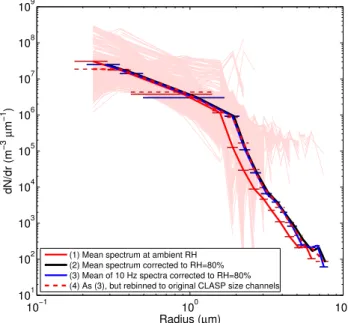
The individual 10 Hz aerosol spectra from a 20-min data record are very variable, particularly in the larger CLASP size channels, and most have a spectral shape very differ-ent to that of the mean spectrum (Fig. 1). This is due to the discrete nature of aerosol measurements and the relatively small volume (5 mL) of each 10 Hz measurement. The black line in Fig. 1 shows this mean spectra once it has been cor-rected from the run-mean relative humidity (60 %) to a ref-erence humidity of 80 %. The blue line in Fig. 1 shows the mean of the 12 000 10 Hz spectra once they have been in-dividually corrected to 80 % relative humidity via a 10 Hz humidity measurement collocated with the CLASP instru-ment. Note that after this procedure, each of these spectra is defined over a different set of channel limits, depending on the sign and magnitude of the individual relative humid-ity adjustment. This mean spectrum is, thus, defined over the mean channel limits of the high-rate aerosol spectra. While this is not useful for any analysis, it does show that before re-binning, correcting for humidity before time-averaging pro-duces an almost identical spectrum to that produced by hu-midity correcting a run-mean aerosol spectrum. The dashed red line in Fig. 1 shows the mean of the high-rate spec-tra after they have been both corrected for relative humid-ity fluctuations and re-binned back to the original CLASP size channels at 10 Hz. This mean spectrum is almost iden-tical to the other two mean adjusted spectra, showing that

10−1 100 101

101 102 103 104 105 106 107 108 109

Radius (µm)

dN/dr (m

−3

µ

m

−1

)

(1) Mean spectrum at ambient RH (2) Mean spectrum corrected to RH=80% (3) Mean of 10 Hz spectra corrected to RH=80% (4) As (3), but rebinned to original CLASP size channels

Fig. 1.An example of using the high-rate relative humidity correc-tion technique described here. The pale red lines show the 12 000 in-dividual spectra which were measured at 10 Hz by the CLASP unit. The solid red line show the mean of these spectra at the mean am-bient relative humidity. The black line shows the mean spectra cor-rected from the mean relative humidity (60 %) to a reference humid-ity of 80 %. The blue line shows the mean of the 12 000 individual spectra after each has been adjusted to 80 % relative humidity (note that this spectrum is then defined over the mean channel boundaries of these individual adjusted spectra). The dashed red line shows the mean of the 12 000 spectra once they have been both adjusted to 80 % and re-binned back to the original CLASP channel limits.

(5)

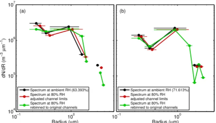
under such an adjustment the largest measurement bin would have to be dropped. Note that adjusting relative humidity to a reference value of 80 % is a rather stringent test of the hu-midity correction algorithm. In practice, if the particle flux in each channel is the same sign, the 10 Hz spectra need only be adjusted to the run-mean relative humidity for the pur-poses of evaluating the flux bias for a single record. The mean flux spectra may then later be adjusted to 80 % humidity (or any other reference value) using standard approaches. In this case, measurements will be corrected to both lower and higher relative humidities, and both the smallest and largest measurement bins must be disregarded. If the particle flux changes sign between size bins, adjustment of the flux spec-trum may be inappropriate and a high-rate correction to the reference humidity required. In this case, channels must be rejected depending on the largest RH adjustment required in this process. It should be noted that, contrary to traditional re-binning methods, which rely on a smooth aerosol spectrum, the high-rate rebinning technique can maintain the spectral shape of a noisy 10 Hz sample (Fig. 2).

2.3 SEASAW Data

The data which are used to test the high rate humidity cor-rections are from cruise D317 (21 March–12 April 2007) of the RRS Discovery made as part of the SEASAW project, a UK contribution to the international SOLAS programme (Brooks et al., 2009; Norris et al., 2012). Three dimensional winds and sonic temperature are available at 20 Hz from a Gill sonic anemometer, pressure and water vapour density are available, also at 20 Hz, from a LI-COR LI-7500 open path gas analyser. Size resolved aerosol spectra are recorded at 10 Hz in 16 unequally spaced channels ranging between radii of 0.18 and 8.88 µm by a CLASP instrument (Hill et al., 2008).

Aerosol, turbulent winds and humidity are time-matched at 10 Hz and split into “runs” of 20 min. These runs are checked to ensure that sonic temperature and momentum flux ogives and relative humidity flux ogives are suitably well be-haved, with a characteristic flattening of the curve at low and high frequencies and a minimal distortion at the wave scale (Fairall et al., 1997). Any runs, where this was not the case, were rejected from the analysis. The run-mean 10 Hz relative humidity timeseries was also required to lie within±10 % of the low-frequency relative humidity from a Vaisala HMP45 humidity probe (part of the ship’s permanent surface me-teorology instrumentation) and all runs, where this was the case, were visually examined to ensure that the LI-COR and low-frequency relative humidity timeseries showed a similar signal. Once this quality control had been carried out, run-mean CLASP aerosol spectra were then visually examined to remove any spectra that were clearly contaminated. This quality control left a total of 124 20-min runs with which to perform the analysis.

10−1 100 104

105 106 107

Radius (µm)

dN/dR (m

−3

µ

m

−1)

(a)

Spectrum at ambient RH (63.393%) Spectrum at 80% RH adjusted channel limits Spectrum at 80% RH rebinned to original channels

10−1 100 Radius (µm)

(a)

(b)

Spectrum at ambient RH (71.613%) Spectrum at 80% RH adjusted channel limits Spectrum at 80% RH rebinned to original channels

Fig. 2.Two examples of a relative humidity correction applied to sea-spray aerosol spectra recorded at 10 Hz. The black lines show the original spectra at ambient humidity, the red lines show these spectra corrected to 80 % relative humidity, and the green lines these corrected spectra after re-binning to the original instrument chan-nels.

3 Functional fits to SEASAW data

Both F84 and K01 assume that, in the mean, an aerosol spec-trum can be well described by a Junge relation of the form

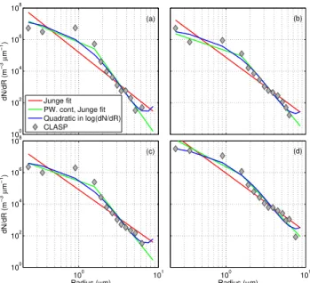
N=αr−(β+1), withβtypically around 3. However, it is not clear that such a relationship is appropriate for the SEA-SAW measured aerosol spectra, which tend to have a smaller change in dN/dr(in log space) with radius at smaller values of r, with a distinct change in gradient at aroundr=1.5– 2 µm, between CLASP channels 4 and 5 (Fig. 3). The green lines in Fig. 3 show Junge fits which are calculated by sub-stituting N∗=log(dN/dr) and r∗=log(r) and finding a linear least-squares fit to N∗ _and _r∗_{. This leaves us with}

N∗₌_br∗₊_a_{and, thus} dN

dr =exp(blog(r)+a) (9)

=earb, (10)

which is a Junge fit withα=eaandβ= −(b+1). This re-sults in a clearly improved fit over the length of the CLASP spectra, with a mean value ofβ over the SEASAW runs of 3.15. However, due to the characteristic shape of the SEA-SAW spectra, this may still result in an overestimation ofN

by over an order of magnitude for small and large values of

r, with an order of magnitude or more underestimation ofN

for values ofrin the middle of the spectrum. Clearly this in not an ideal situation.

Also shown in Fig. 3 are two further functional fits for dN/dr which offer an improvement over the simple log-linear Junge fits. The red line shows a quadratic fit of the form dN/dr=exp

(6)

100 102 104 106 108

dN/dR (m

−3

µ

m

−1)

(a) (b)

100 101 100

102 104 106 108

Radius (µm)

dN/dR (m

−3

µ

m

−1

)

(c)

100 101 Radius (µm)

(d) Junge fit

PW. cont, Junge fit Quadratic in log(dN/dR) CLASP

Fig. 3.Four different fits encompassing three different functional forms to aerosol spectra from four randomly chosen 20-min SEA-SAW runs.

Table 1.Characteristics ofβvalues of different Junge-type fits to the SEASAW data

Mean Min Max σ

Jungeβ 2.708 1.756 5.188 0.440

PW-Jungeβ₁ 1.056 −1.698 2.730 0.709

PW-Jungeβ₂ 5.042 3.341 6.743 0.672

with the F84 and K01 adjustment methods, and will result in different bias velocities for channels 1–4 and 4–16. The log-quadratic fit has the benefit that it is continuously dif-ferentiable and so will result in a unique bias velocity for each CLASP channel, however, it is strictly only valid within the radius range of the CLASP channels, and will diverge quickly from the CLASP recorded spectra outside this range. Using this functional form also complicates the expression for the K01 and F84 bias velocities due to the more compli-cated derivative with respect tor.

The mean error for each CLASP channel resulting from the three functional fits described above are shown in Fig. 4. The left panel shows the absolute error,|Ni−Fi|, whereF is the fit toN, and the right panel shows this error normalised by the channel mean number count,|Ni−Fi|/Ni. The Junge fit performs reasonably well, but introduces a considerable error at the small and large ends of the CLASP spectrum. This Junge fit does perform better than either of the more complicated functional forms for particle sizes of around 2 µm, but this is simply where the function changes from un-derestimating to overestimating the particle count (with in-creasingr). The piecewise-linear and log-quadratic fits both perform similarly, and it is not immediately obvious from

100

101

100

102

104

106

108

1010

Radius (µm)

Error (m

−3

µ

m

−1)

(a) Junge fit

PW. cont. Junge fit Quadratic in log(dN/dR)

100

101

10−2

10−1

100

101

102

Radius (µm)

Relative error

(b) Junge fit

PW. cont. Junge fit Quadratic in log(dN/dR)

Fig. 4.Mean absolute (a) and relative (b) errors for the fits shown in Fig. 1. The relative errors are simply the absolute error normalised

by the mean particle count,N. The triangles in (a) indicate whether

the mean error is positive or negative.

20 40 60 80 100 120

0 0.01 0.02 0.03 0.04

∆

vd

(m s

−1)

(a)

20 40 60 80 100 120

0 0.002 0.004 0.006 0.008 0.01

Sat. ratio flux (m s

−1)

Run # (b)

F84 ∆v_d K01 ∆v_d

c_p1/2u_*(1−S) <S′w′>

Fig. 5.(a) Run-by-run comparison of K01 and F84 methods for

calculating bias velocity,1v_d; (b) Run-by-run comparison of

satu-ration ratio flux and the F84 approximation to it.

Fig. 4 which provides the best fit. We can calculate this more objectively by summing the relative errors over the CLASP channels. This gives a value of 10.9 for the piecewise-linear Junge fit and 9.2 for the log-quadratic fit, suggesting that the latter provides, on average, a superior fit to the CLASP spec-tra than does the piecewise-Junge fit. However, as the error metric for both of these fits are similar, we will consider both of these later.

4 Bulk methods for calculating bias velocity

The K01 and F84 bias velocities, 1v_d, given by Eqs. (5) and (7), respectively, both give similar, physically rea-sonable (Fig. 5a). However, K01’s method (mean = 0.010,

σ= 0.0069) is generally more variable and very slightly smaller than F84’s method (mean = 0.011, σ= 0.0040). Given that the only difference between the K01 and F84 methods is F84’s approximation ofw′_S′_as_c1/2

(7)

20 40 60 80 100 120 0

0.02

0.04 Channel 2: r=0.29−0.41µm

Δ

vd

(m s

−1)

Run #

20 40 60 80 100 120 0

0.02

0.04 Channel 3: r=0.41−1.4µm

Run #

Δ

vd

(m s

−1)

High−rate Δv_d F84 Δv

d

K01 Δv

d

20 40 60 80 100 120 0

0.02 0.04

0.06 Channel 4: r=1.4−1.7µm

Δ

vd

(m s

−1

)

Run #

20 40 60 80 100 120 0

0.02 0.04 0.06 0.08

0.1 Channel 5: r=1.7−2.1µm

Δ

vd

(m s

−1

)

Run #

20 40 60 80 100 120 0

0.02 0.04 0.06 0.08 0.1

Channel 6: r=2.1−2.4µm

Δ

vd

(m s

−1

)

Run #

20 40 60 80 100 120 0

0.02 0.04 0.06 0.08 0.1

Δ

vd

(m s

−1

)

Run #

20 40 60 80 100 120 0

0.02 0.04 0.06 0.08 0.1

Δ

vd

(m s

−1

)

Run #

20 40 60 80 100 120 −0.05

0 0.05 0.1

Δ

vd

(m s

−1

)

Run #

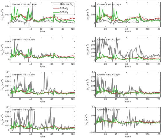
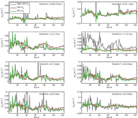
Fig. 6.Apparent deposition velocity due to hygroscopicity,1v_d, calculated through K01’s and F84’s methods, and the difference in the high-rate deposition velocity between ambient and RH-corrected (to run mean) spectra. CLASP channels 2–9 are shown.

it. Where there is a significant saturation flux, F84’s method tends to underestimate the saturation ratio flux by up to 50 %. Where the saturation ratio is smaller, however, the F84 ap-proximation may overestimate by a similar margin.

5 Comparison of bulk and high-rate bias estimates

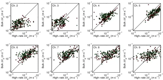
A comparison of the apparent deposition velocity,1vd,

be-tween the K01 and F84 methods and the high-rate method is shown in Fig. 6 for CLASP channels 2–9. Note that in the K01 and F84 methods,1vddoes not depend on particle

ra-dius, so only the high-rate1vdis changing in each of these

plots. In channels 2 and 3 the bias velocity from the bulk methods is comparable to that from the high-rate corrections, however, in general they are biased significantly high. This is unsurprising given the assumption that the aerosol spec-trum follows a single Junge law (withβ≈3), whereas, as we saw in Fig. 3, the SEASAW spectra generally have a much shallower gradient than this in channels 1–4, and a steeper gradient for channels 4–16. Using β=3 for the bulk ap-proximations will, thus, inevitably lead to an overestimation of the bias velocity. There are some notable changes in the

relationship between bulk and high-rate deposition velocity errors between channels (Fig. 7). These are discussed later.

In CLASP channel 4, the bulk1vd, particularly from the

K01 method, matches extremely closely with that derived from the high-rate method. Generally, it is around channel 4 where the CLASP aerosol spectrum steepens from a gra-dient of around 1.5 to around 5 (Table 1). Thus, the mean gradient across channel 4 is only slightly larger than 3 so the bulk methods would be expected to perform well here, pro-viding other assumptions and approximations on which these rely are met. Note that the K01 method makes fewer approx-imations than the F84 method does – namely the use ofw′_S′ rather than an estimate of it – explaining why it generally performs better. This is particularly pronounced in channel 4.

In channels 5–16 theβ-value in the CLASP aerosol spec-tra increases to typically around 5, so the assumption that

β≈3 again fails, this time resulting in the bulk methods underestimating 1vd. This is most pronounced in CLASP

(8)

10−3 10−2 10−1 10−3

10−2 10−1

High−rate ∆V_d (m s

−1) Bulk ∆ Vd (m s −1) Ch. 2

10−3 10−2 10−1 10−3

10−2 10−1

−1) Bulk ∆ Vd (m s −1) Ch. 3

10−3 10−2 10−1 10−3

10−2 10−1

−1) Bulk ∆ Vd (m s −1) Ch. 4

10−3 10−2 10−1 10−3

10−2 10−1

−1) Bulk ∆ Vd (m s −1) Ch. 5

10−3 10−2 10−1 10−3

10−2 10−1

−1) Bulk ∆ Vd (m s −1) Ch. 6

10−3 10−2 10−1 10−3

10−2 10−1

−1) Bulk ∆ Vd (m s −1) Ch. 7

10−3 10−2 10−1 10−3

10−2 10−1

−1) Bulk ∆ Vd (m s −1) Ch. 8

10−3 10−2 10−1 10−3

10−2 10−1

−1) Bulk ∆ Vd (m s −1) Ch. 9 K01 F84

Fig. 7.Scatterplots showing the relationships between CLASP1v_dand K01/F841v_din Fig. 6

20 40 60 80 100 120

102

103

104

105

106

Bias flux (m

−2

s

−1

)

Run #

20 40 60 80 100 120

101 102 103 104 105 106

Bias flux (m

−2

s

−1

)

Run #

20 40 60 80 100 120

102

103

104

105

Run #

Bias flux (m

−2 s −1 ) High−rate Bias F84 Bias K01 Bias

20 40 60 80 100 120

101

102

103

104

105

Bias flux (m

−2

s

−1

)

Run #

20 40 60 80 100 120

100 101 102 103 104 105

Bias flux (m

−2

s

−1

)

Run #

20 40 60 80 100 120

100 101 102 103 104 105

Bias flux (m

−2

s

−1

)

Run #

20 40 60 80 100 120

101

102

103

104

105

Bias flux (m

−2

s

−1

)

Run #

20 40 60 80 100 120

100

101

102

103

Bias flux (m

−2

s

−1

)

Run #

Fig. 8.Flux bias due to hygroscopicity, (=1v_dN|_RH), calculated through K01’s and F84’s methods, and the difference in the high-rate

number flux,N′_w′_{, between raw and RH-corrected (to run mean) spectra. Black crosses indicate a negative high-rate flux bias. CLASP}

channels 2–9 are shown.

comparison with the unchanging bulk methods less useful (this is likely due to a decreasing signal-to-noise ratio as fewer and fewer particles are recorded in the larger CLASP channels).

The bias velocity,1vd, is not a true deposition velocity,

but an artifact of measuring size-resolved hygroscopic parti-cle concentration in the presence of a humidity flux. How-ever, this apparent deposition will lead to an error in the

calculation of the particle fluxw′_N′_{, by an amount equal to}

1vdN_RH, where the RH subscript indicates thatN has been

(9)

20 40 60 80 100 120 0

0.02

0.04 Channel 2: r=0.29−0.41µm

Run #

Δ

vd

(m s

−1

)

High−rate Δv

d

F84 Δv

d

K01 Δv

d

20 40 60 80 100 120 −0.01

0 0.01 0.02

Δ

vd

(m s

−1

)

Run #

20 40 60 80 100 120 0

0.02 0.04

0.06 Channel 4: r=1.4−1.7µm

Δ

vd

(m s

−1

)

Run #

20 40 60 80 100 120 0

0.02 0.04 0.06 0.08

0.1 Channel 5: r=1.7−2.1µm

Δ

vd

(m s

−1

)

Run #

20 40 60 80 100 120 0

0.02 0.04 0.06 0.08 0.1

Δ

vd

(m s

−1

)

Run #

20 40 60 80 100 120 0

0.02 0.04 0.06 0.08 0.1

Δ

vd

(m s

−1

)

Run #

20 40 60 80 100 120 0

0.02 0.04 0.06 0.08 0.1

Δ

vd

(m s

−1

)

Run #

20 40 60 80 100 120 −0.05

0 0.05 0.1 0.15

Δ

vd

(m s

−1

)

Run #

Fig. 9.Apparent deposition velocity due to hygroscopicity,1v_d, calculated through K01’s and F84’s methods, modified to use a piecewise (log-)linear Junge form, and the difference in high-rate deposition velocity between raw and RH-corrected (to run mean) spectra. CLASP channels 2–9 are shown.

the bulk method, particularly from the K01 method, match the high-rate method well (Fig. 8). Where they are in error, they are generally biased high; this is particularly clear in CLASP channel 2 from around run 85 onwards, roughly cor-responding to where the saturation ratio flux becomes small. There are also times when the high-rate flux bias is negative, which the bulk methods cannot reproduce for observed val-ues ofβ. Note that a negative flux bias may occur in a posi-tive humidity flux as a result of the shape of the aerosol spec-trum. If the spectrum is relatively flat for small values ofr, then the expansion of the channel limits under increasing hu-midity may cause a loss of particles for certain size channels, even when adjusting to higher relative humidities. A negative bias flux may also result if the spectral shape or mean number concentration is correlated with relative humidity. This may occur as fresh plumes of sea spray (withN′>0) increase the local ambient relative humidity through droplet evaporation. Such a situation would also invalidate the assumption of F84 and K01 that the dry aerosol distribution is well mixed and uncorrelated with relative humidity.

5.1 Bulk methods based on improved functional forms

5.1.1 A piecewise linear Junge power law

Given the characteristic shape of the aerosol spectra in the SEASAW dataset, the use of a single Junge power law to approximate the spectra, as suggested by F84 and K01 is not particularly appropriate. An obvious improvement that can be made to this is to use two Junge-type fits: one be-tween channels 1 and 4 where the CLASP spectra are gen-erally quite shallow, and another between channels 4 and 16 where the spectra steepen, modified so these fits produce one piecewise-continuous fit. This gives us different values forβ

for channels 1–3 and 5–16 which can then be used in the F84 and K01 expressions for the bias velocity. Due to the change of gradient at channel 4,βis undefined here, so we must use a mean of the twoβvalues on either side. Generally this will give a value ofβ≈3 at channel 4. Examples of this type of fit are shown overlying CLASP spectra in Fig. 3.

5.1.2 Quadratic fit in log(dN/dr), r

(10)

10−3 10−2 10−1 10−3

10−2 10−1

High−rate ∆Vd (m s −1 ) Bulk ∆ Vd (m s −1

) Ch. 2

10−3 10−2 10−1 10−3

10−2 10−1

) Ch. 3

10−3 10−2 10−1 10−3

10−2 10−1

) Ch. 4

10−3 10−2 10−1 10−3

10−2 10−1

) Ch. 5

10−3 10−2 10−1 10−3

10−2 10−1

−1 ) Bulk ∆ Vd (m s −1

) Ch. 6

10−3 10−2 10−1 10−3

10−2 10−1

−1 ) Bulk ∆ Vd (m s −1

) Ch. 7

10−3 10−2 10−1 10−3

10−2 10−1

−1 ) Bulk ∆ Vd (m s −1

) Ch. 8

10−3 10−2 10−1 10−3

10−2 10−1

−1 ) Bulk ∆ Vd (m s −1

) Ch. 9

Fig. 10.Scatterplots showing the relationships between the high-rate1v_dand modified K01 (red) and F84 (green)1v_din Fig. 9.

20 40 60 80 100 120 0

0.02 0.04

Run #

Δ

vd

(m s

−1)

High−rate Δv_d Quadratic Δv

d

20 40 60 80 100 120 −0.01

0 0.01 0.02 0.03

Δ

vd

(m s

−1)

Run #

20 40 60 80 100 120 0

0.02 0.04 0.06

Δ

vd

(m s

−1)

Run #

20 40 60 80 100 120 0

0.02 0.04 0.06 0.08

0.1 Channel 5: r=1.7−2.1

µm Δ vd (m s −1) Run #

20 40 60 80 100 120 0 0.02 0.04 0.06 0.08 0.1

Δ vd (m s −1 ) Run #

20 40 60 80 100 120 0 0.02 0.04 0.06 0.08 0.1

Fig. 11.Apparent deposition velocity due to hygroscopicity,1vd, calculated through K01’s method, modified to use a log-linear quadratic functional form, and the difference in high-rate deposition velocity between raw and RH-corrected (to run mean) spectra. CLASP channels 2–9 are shown.

function which is continuously dependent on particle radius. For example, if we fit a quadratic in log(dN/dr),r space, then we end up with a functional representation of the aerosol spectrum of the form

dN

dr =exp n

ar2+br+co.

Again, examples of this fit are shown along with CLASP measured spectra in Fig. 3. Following K01, we may then derive a bias velocity which is continuously dependent on particle radius,r. This gives us

1vd=

γ 2ar2+br+1

3(1−S)(1−S+γ )w

(11)

10−3 10−2 10−1 10−3

10−2 10−1

−1₎

Quadratic K01

∆

Vd

(m s

−1

)

Ch. 2

10−3 10−2 10−1 10−3

10−2 10−1

−1₎

Quadratic K01

∆

Vd

(m s

−1

)

Ch. 3

10−3 10−2 10−1 10−3

10−2 10−1

−1₎

Quadratic K01

∆

Vd

(m s

−1

)

Ch. 4

10−3 10−2 10−1 10−3

10−2 10−1

−1₎

Quadratic K01

∆

Vd

(m s

−1

)

Ch. 5

10−3 10−2 10−1 10−3

10−2 10−1

−1₎

Quadratic K01

∆

Vd

(m s

−1

)

Ch. 6

10−3 10−2 10−1 10−3

10−2 10−1

−1₎

Quadratic K01

∆

Vd

(m s

−1

)

Ch. 7

10−3 10−2 10−1 10−3

10−2 10−1

−1₎

Quadratic K01

∆

Vd

(m s

−1

)

Ch. 8

10−3 10−2 10−1 10−3

10−2 10−1

−1₎

Quadratic K01

∆

Vd

(m s

−1

)

Ch. 9

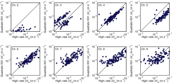
Fig. 12.Scatterplots showing the relationships between high-rate1v_dand K01 (modified to use a log-linear quadratic fit)1v_din Fig. 11.

102

103

104

105

106

102

103

104

105

106

(a) Channel 3

r=0.41−1.40µm

Corrected flux (bulk, m−2_s−1₎

Corrected flux (high−rate, m

−2

s

−1

)

101

102

103

104

105

101

102

103

104

105

−2

s

−1

)

(b) Channel 5

r=1.75−2.05µm F84K01

PW−linear K01 Quadratic K01

100 101 102 103 104 105

100

101

102

103

104

105

(c) Channel 7

r=2.42−2.84µm

−2

s

−1

)

10−1 100 101 102 103

10−1

100

101

102

103

(d) Channel 9

r=3.22−3.59µm

−2

s

−1

)

Fig. 13.Comparisons of the high-rate and bulk corrected fluxes for CLASP channels 3, 5, 7 and 9. Upward and downward pointing triangles show where both the high-rate and bulk fluxes are positive or negative, respectively. The lighter points show fluxes of different sign, for positive (circle) and negative (square) high-rate fluxes.

5.2 Do these adjusted methods offer an improvement?

Timeseries and scatter-plots showing the relationship be-tween the high-rate corrections and the piecewise-Junge F84 and K01 methods are shown in Figs. 9 and 10, respectively. Using the piecewise continuous Junge fits in place of a single Junge fit is essentially equivalent to multiplying1vd from

(12)

effect of tempering the usual overestimation of1v_din chan-nels 1–3 and the underestimation in chanchan-nels 5–16. How-ever, despite the piecewise continuous Junge fits producing a generally very good approximation of the SEASAW aerosol spectra, there are still times when there are significant dif-ferences between the bulk and high-rate methods, suggesting that variables not considered within the bulk methods may be important.

Using K01’s method, modified to use a quadratic fit to the CLASP aerosol spectra (Figs. 11 and 12), offers a similar im-provement to the estimation of the bias velocity over the stan-dard K01 and F84 bulk methods, particularly at the smaller end of the spectra where the quadratic fit can represent the complete flattening of the spectra which is sometimes ob-served in the SEASAW aerosol data. The two distinct group-ings visible in channel 3 are related to a change in mete-orological conditions (particularly the humidity flux) from around run 84 onwards. Before this time, the bulk method tends to overestimate the deposition velocity error and af-ter this time the deposition velocity error is underestimated. This is also apparent, albeit to a much lesser extent and in the opposite sense in channels 4 and 5. This difference is ex-aggerated in channel 3 because this channel is much wider (in a logarithmic sense) than any of the other channels (see, for example, Fig. 1). The bias apparent in channel 5 is mainly due to a consistent underestimation of the slope of the aerosol spectra by the quadratic fit. It is clear from Fig. 3 that the gra-dients of the measured spectra tend to increase significantly in gradient between channels 4 and 5. Such a sharp increase in gradient tends to be underestimated by the functional fit to the spectra (particularly in the case of the smoothly vary-ing quadratic form considered here). The bulk estimates are linearly dependent on the gradient of the aerosol spectra, thus, this underestimation of the gradient leads to a system-atic bias in the deposition velocity error. At larger particle sizes, counting statistics become poor and the eddy covari-ance method becomes an increasingly less valid method of determining aerosol fluxes. This is reflected by the increas-ingly poor correlations in the larger channels, particularly in channel 9.

Although both the piecewise-Junge and quadratic forms of the K01 correction generally allow an improved bulk repre-sentation of the bias velocity (and resulting bias flux) it is clear that no one method is superior under all circumstances seen in the SEASAW data; indeed there are times when the simple Junge fit presented by K01 offers the best approx-imation to the “true” bias velocity calculated through our high-rate method. Furthermore, there are times when none of the bulk methods considered here provide a suitable approx-imation of the hygroscopicity-induced bias suggested by the high-rate method. This can be clearly seen in Fig. 13, where comparisons of the particle number fluxes,N′_w′_{, corrected} using our high-rate method and using the various bulk meth-ods discussed here are shown for CLASP channels 3, 5, 7 and 9.

6 Conclusions

The use of the eddy covariance technique to measure the size-segregated flux of sea-spray aerosol (or other hygro-scopic aerosol) in the presence of a relative humidity flux may lead to a significant systematic bias in the recorded flux. “Bulk” methods (F84 & K01) have been presented to account for this bias using mean meteorological conditions (F84) or turbulent measurements (K01) and an assumed mean shape of the aerosol spectra, in the form of a Junge power law.

In this paper, we have developed a method for correcting aerosol spectra for variations in relative humidity at the high temporal resolution required for the calculation of eddy co-variance fluxes, allowing the flux bias caused by the relative humidity flux to be explicitly calculated. We have also re-formulated the corrections given by F84 and K01 to use a more representative shape of the mean aerosol spectra. In sit-uations where turbulent (high-rate) measurements of humid-ity are not available and aerosol spectra have not been dried, the bulk correction described by F84 provides a reasonable estimation of the flux correction which must be applied to account for the effects of hygroscopicity. If turbulent mea-surements of humidity are available, then the bulk correction of K01 offers an improvement, particularly when modified to better model the shape of the mean aerosol spectra. How-ever, these bulk methods are far from infallible and may, at times, significantly under or overestimate the required flux correction. In situations where collocated turbulent aerosol and humidity measurements are available, the high-rate cor-rection method is recommended, despite the relatively high computational cost.

Acknowledgements. SEASAW was funded by the UK Natural

En-vironment Research Council, grant number NE/C001842/1 as part of UK-SOLAS. DAJS was funded by NERC grant NE/H004238/1. We would like to thank two anonymous reviewers whose comments have helped improve this manuscript.

Edited by: A. Stoffelen

References

Andreas, E. L.: Sea Spray and the Turbulent Air-Sea Heat Fluxes, J. Geophys. Res., 97, 11429–11441, 1992.

Andreas, E. L.: A new sea spray generation function for wind speeds

up to 32 m s−1, J. Phys. Oceanogr., 28, 2175–2184, 1998.

Andreas, E. L.: A review of the sea spray generation function for the open ocean, in: Atmosphere-Ocean Interactions, edited by: Perrie, W., Vol. 1, 1–46, WIT Press, 2002.

Andreas, E. L., Jones, K. F., and Fairall, C. W.: Production ve-locity of sea spray droplets, J. Geophys. Res., 115, C12065, doi:10.1029/2010JC006458, 2010.

(13)

DeGrandpre, M., Dixon, J., Drennan, W. M., Gabriele, J., Gold-son, L., Hardman-Mountford, N., Hill, M. K., Horn, M., Hsueh, P.-C., Huebert, B., de Leeuw, G., Leighton, T. G., Liddicoat, M., Lingard, J. J. N., McNeil, C., McQuaid, J. B., Moat, B. I., Moore, G., Neill, C., Norris, S. J., O’Doherty, S., Pascal, R. W., Prytherch, J., Rebozo, M., Sahlee, E., Salter, M., Schuster, U., Skjelvan, I., Slagter, H., Smith, M. H., Smith, P. D., Srokosz, M., Stephens, J. A., Taylor, P. K., Telszewski, M., Walsh, R., Ward, B., Woolf, D. K., Young, D., and Zemmelink, H.: Physical Ex-changes at the Air-Sea Interface: Field Measurements from UK-SOLAS, B. Am. Meteorol. Soc., 90, 629–644, 2009.

Clarke, A. D., Owens, S. R., and Zhou, J.: An ultra fine sea-salt flux from breaking waves: Implications for cloud condensation nuclei in the remote marine atmosphere, J. Geophys Res., 111, D06202, doi:10.1029/2005JD006565, 2006.

de Leeuw, D., Andreas, E. L., Anguelova, M. D., Fairall, C. W., Lewis, E. R., O’Down, C., Schulz, M., and Schwartz, S. E.: Pro-duction flux of sea spray aerosol, Rev. Geophys., 49, RG2001, doi:10.1029/2010RG000349, 2011.

de Leeuw, G., Moerman, M., Cohen, L., Brooks, B., Smith, M., and Vignati, E.: Aerosols, bubbles and sea spray production studies during the RED experiments, in: AMS conference, 2003. de Leeuw, G., Moerman, M., Zappa, C. J., McGillis, W. R.,

Nor-ris, S. J., and Smith, M. H.: Eddy Correlation Measurements of Sea Spray Aerosol Fluxes, in: Transport at the Air Sea Interface, edited by: Garbe, C. S., Handler, R. A., and J¨ahne, B., Springer-Verlag, 2007.

Doss-Hammel, S. M., Zeisse, C. R., Barrios, A. E., de Leeuw, G., Moerman, M., de Jong, A. N., Frederickson, P. A., and David-son, K. L.: Low-altitude Infrared Propagation in a Coastal Zone: Refraction and Scattering, Appl. Optics, 41, 3706–3724, 2002. Fairall, C. W.: Interpretation of eddy-correlation measurements of

particulate deposition and aerosol flux, Atmos. Environ., 18, 1329–1337, 1984.

Fairall, C. W. and Larsen, S. E.: Dry deposition, surface production and dynamics of aerosols in the marine boundary layer, Atmos. Environ., 18, 69–77, 1984.

Fairall, C. W., Davidson, K. L., and Schaucher, G. E.: An analysis of the surface production of sea-salt aerosol, Tellus B, 35, 31–39, 1983.

Fairall, C. W., White, A. B., Edson, J. B., and Hare, J. E.: Integrated shipboard measurements of the marine boundary layer, Atmos. Ocean. Tech., 14, 338–359, 1997.

Geever, M. C., O’Dowd, D., van Ekeren, S., Flanagan, R.,

Nilsson, E. D., de Leeuw, G., and Ranmik, ¨U.:

Submi-cron sea spray fluxes, Geophys. Res. Lett., 32, L15810, doi:10.1029/2005GL023081, 2005.

Haywood, J. M., Ramaswamy, V., and Soden, B. J.: Tropospheric aerosol climate forcing in clear-sky satellite observations over the oceans, Science, 283, 1299–1393, 1999.

Hill, M. K., Brooks, B. J., Norris, S. J., Smith, M. H., Brooks, I. M., de Leeuw, G., and Lingard, J. J. N.: A Compact Lightweight Aerosol Spectrometer Probe (CLASP), J. Atmos. Oceanic Tech., 25, 1996–2006, doi:10.1175/2008JTECHA1051.1, 2008. Hoppel, W. A., Frick, G. M., and Fitzgerald, J. W.: The surface

source function for sea-salt aerosol and aerosol dry deposition to the ocean surface, J. Geophys. Res., 107, 4382–4399, 2002.

Junge, C. E.: Air Chemistry and Radioactivity, Academic Press, New York, 1963.

Kowalski, A. S.: Deliquescence induces eddy covariance and es-timable dry deposition errors, Atmos. Environ., 35, 4843–4851, doi:10.1016/S1352-2310(01)00270-9, 2001.

Large, W. G. and Pond, S.: Open ocean momentum flux measure-ments in moderate to strong winds, J. Phys. Oceanogr., 11, 324– 336, 1981.

Lewis, E. R. and Schwartz, S. E.: Comment on “Size distribution of sea-salt emissions as a function of relative humidity”, Atmos. Environ., 40, 588–590, 2003.

M˚artensson, E. M., Nilsson, E. D., de Leeuw, G., Cohen, L. H., and Hansson, H. C.: Laboratory simulations and parameterization of the primary marine aerosol production, J. Geophys. Res., 108, 4927, doi:10.1029/2002JD002263, 2003.

Monahan, E. C., Spiel, D. E., and Davidson, K. L.: Whitecap aerosol productivity deduced from simulation tank measure-ments, J. Geophys. Res., 87, 8898–8904, 1982.

Monahan, E. C., Spiel, D. E., and Davidson, K. L.: A model of marine aerosol generation via whitecaps and wave disruption, in: Oceanic Whitecaps, edited by: Monahan, E. C. and Niocaill, G. M., 167–174, D. Reidel Publishing Company, 1986.

Nilsson, E. D., Ranmik, ¨U., Swietliki, E., Leck, C., Aalto, P. P.,

Zhou, J., and Norman, M.: Turbulent aerosol fluxes over the Arc-tic Ocean: 2. Wind driven sources from the sea, J. Geophys. Res., 106, 32139–32154, 2001.

Norris, S. J., Brooks, I. M., de Leeuw, G., Smith, M. H., Moerman, M., and Lingard, J. J. N.: Eddy covariance measurements of sea spray particles over the Atlantic Ocean, Atmos. Chem. Phys., 8, 555–563, doi:10.5194/acp-8-555-2008, 2008.

Norris, S. J., Brooks, I. M., Hill, M. K., Brooks, B. J., Smith, M. H., and Sproson, D. A. J.: Eddy Covariance Measurements of the Sea Spray Aerosol Flux over the Open Ocean, J. Geophys. Res., 117, D07210, doi:10.1029/2011JD016549, 2012.

Petelski, T. and Piskozub, J.: Vertical coarse aerosol fluxes in the atmospheric surface layer over the North Polar Waters of the Atlantic, J. Geophys. Res., 111, C06039, doi:10.1029/2005JC003295, 2006.

Reid, J. S., Jonsson, H. H., Smith, M. H., and Smirnov, A.: Evolu-tion of te Vertical Profile and Flux of Large Sea-Salt Particles in a Coastal Zone, J. Geophys. Res., 106, 12039–12053, 2001. Smith, M. H., Park, P. M., and Consterdine, I. E.: Marine aerosol

concentrations and estimated fluxes over the ocean, Q. J. Roy. Meteorol. Soc., 115, 809–824, 1993.

Vignati, E., de Leeuw, G., and Berkowicz, R.: Modeling coastal aerosol transport and effects of surf-produced aerosols on pro-cesses in the marine atmospheric boundary layer, J. Geophys. Res., 106, 20225–20238, 2001.

Yelland, M. J., Moat, B. I., Taylor, P. K., Pascal, R. W., Hutch-ings, J., and Cornell, V. C.: Wind stress measurements from the open ocean corrected for airflow distortion by the ship, J. Phys. Oceanogr., 28, 1511–1526, 1998.