THE IMPACT OF SEA LEVEL RISE ON GEODETIC VERTICAL DATUM OF PENINSULAR MALAYSIA

THE IMPACT OF SEA LEVEL RISE ON GEODETIC VERTICAL DATUM OF

PENINSULAR MALAYSIA

A H M Din a,b*, I C Abazu a, M F Pa’suya a,c ,K M Omar a and A I A Hamid a a

Geomatic Innovation Research Group (GIG), Faculty of Geoinformation and Real Estate, Universiti Teknologi Malaysia, 81310 Johor Bahru, Johor, Malaysia.

b

Geoscience and Digital Earth Centre (INSTEG), Universiti Teknologi Malaysia, 81310 Johor Bahru, Johor, Malaysia. c

Faculty of Architecture, Planning and Surveying, Department of Surveying Science and Geomatics, Universiti Teknologi Mara Perlis, Arau, Perlis, Malaysia.

*amihassan@utm.my

KEY WORDS: Sea Level Rise, Tide Gauge, Satellite Altimeter, Geodetic Vertical Datum

ABSTRACT:

Sea level rise is rapidly turning into major issues among our community and all levels of the government are working to develop responses to ensure these matters are given the uttermost attention in all facets of planning. It is more interesting to understand and investigate the present day sea level variation due its potential impact, particularly on our national geodetic vertical datum. To determine present day sea level variation, it is vital to consider both in-situ tide gauge and remote sensing measurements. This study presents an effort to quantify the sea level rise rate and magnitude over Peninsular Malaysia using tide gauge and multi-mission satellite altimeter. The time periods taken for both techniques are 32 years (from 1984 to 2015) for tidal data and 23 years (from 1993 to 2015) for altimetry data. Subsequently, the impact of sea level rise on Peninsular Malaysia Geodetic Vertical Datum (PMGVD) is evaluated in this study. the difference between MSL computed from 10 years (1984 – 1993) and 32 years (1984 – 2015) tidal data at Port Kelang showed that the increment of sea level is about 27mm. The computed magnitude showed an estimate of the long-term effect a change in MSL has on the geodetic vertical datum of Port Kelang tide gauge station. This will help give a new insight on the establishment of national geodetic vertical datum based on mean sea level data. Besides, this information can be used for a wide variety of climatic applications to study environmental issues related to flood and global warming in Malaysia.

1. RESEARCH BACKGROUND

Sea level rise are rapidly turning into major issues among our community and all levels of the government are working to develop responses to ensure these matters are given the uttermost attention in all facets of planning. The release of the fourth assessment report of the Intergovernmental Panel on Climate Change (IPCC) in 2007 was followed by much debate both in the media and the scientific community, especially on the sea level rise issues (Meehl et al., 2007). This was due to the fact that sea level rise is one of the most devastating effects of global climate change that will have far-reaching consequences for a majority of the world’s population and natural system. Although there is great uncertainty about the rates, range and specific time periods in which sea levels will increase (IPCC, 2007; Solomon et al., 2007; Horton et al., 2008; Pittock, 2009), currently sea level rise is becoming one of the most imperative impacts of climate change, which will progress well beyond the 21st century (Nicholls and Tol, 2006; IPCC, 2007; Vermeer and Rahmstorf, 2009; Woodard et al., 2010; Schaeffer et al., 2012).

It is more interesting to understand and investigate the present day sea level variation due its potential impact particularly on our national geodetic vertical datum. To determine present day sea level variation, it is vital to consider both in-situ tide gauge and remote sensing measurements. The advantage of the traditional tide gauge measurements is that they provide relatively long time series, while satellite altimeter mission data were only available commencing after 1992. Tide gauge is the primary measurement of sea level variation prior to 1990s. Currently, there are 21 tide gauges installed in Malaysia by Department of Survey and Mapping Malaysia (DSMM). With

the launch of the satellite altimeter technology in late 1992, it has proven that it has a good potential as a complementary tool to the traditional coastal tide gauge instruments for monitoring sea level changes, particularly for the deep ocean.

Sea level change refers to the change in mean sea level over time in response to global climate and local tectonic changes. Sea level is the height of the sea surface with respect to a vertical control point, or benchmark. However, change in sea level relative to land (local mean sea level change) can be significantly different from the global mean sea level (GMSL) change because of changes in the distribution of water in the ocean and vertical movement of the land. In Peninsular Malaysia, DSMM embarked on a project for the determination of precise mean sea level in 1983 by involving 12 tide gauge observations and it was known as Tidal Observation Network (TON). In the project, a tide gauge station at Port Kelang was chosen for adoption of Peninsular Malaysia Geodetic Vertical Datum (PMGVD). The PMGVD is based on 10 years of tidal observations at Port Kelang from 1984 to 1993 by adopting Mean Sea Level (MSL) at 3.624m above zero tide gauge as the reference level (Mohamed, 2003; Sulaiman, 2016).

of national geodetic vertical datum based on mean sea level data. Besides, this information can be used for a wide variety of climatic applications to study environmental issues related to flood and global warming in Malaysia.

1.1 Tide Gauge

A tide gauge is a simple graduated staff or other reference on which the water level can be visually identified. The setting-up of tide gauge is to estimate a continuous time series of sea level. This technique has been used to determine the water level as far back as the 17th century. Tidal observations via tide gauge can be surprisingly accurate if carefully and faithfully executed. However, to be useful for most investigations of climate change, a record of water levels should be temporally long and dense (the longer the better). In addition, the record must maintain internal consistency in spite of repairs, replacements, and changes of tide gauge technology.

Generally, a tide gauge record tides, effects of ocean circulation, meteorological forcing of water, local or regional uplift or subsidence at the measurement site and errors inherent to the gauges. With so many factors involved in maintaining a consistent record over an extended time such as a century or more, a cooperative international program is necessary. The Permanent Service for Mean Sea Level (PSMSL) has been responsible for the collection, publication, analysis and interpretation of sea level data from the global network of tide gauges since 1933. The PSMSL centre is based at the Proudman Oceanographic Laboratory in United Kingdom. The PSMSL manages sea level data from nearly 200 national authorities. The tidal data can be accessed freely through http://www.psmsl.org/.

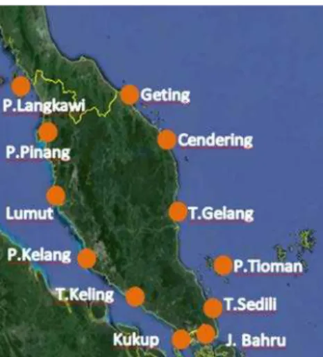
In Malaysia, the Department of Survey and Mapping Malaysia (DSMM) is the main government agency in Malaysia responsible for the acquisition, processing, archiving, and dissemination of tidal data. DSMM is also responsible to submit all tide gauge station data in Malaysia to PSMSL in monthly and yearly average. Currently, there are 12 tidal stations along the coast of Peninsular Malaysia (West Malaysia) and 9 tidal stations along the coast of Sabah and Sarawak (East Malaysia). For the purpose of this study, only tidal stations in Peninsular Malaysia are involved. The period of the tidal data starts from 1984 up to 2015. Figure 1 shows the distribution of tide gauge stations in Peninsular Malaysia.

Figure 1. The distribution of tide gauge stations in Peninsular Malaysia that was employed in this study

Each tide gauge station in Malaysia consists of a tide gauge protective house, stilling or tide well, tide staff and several reference benchmarks, one of which is referred to as the tide gauge bench mark (Mohamed, 2003). The tide gauge measures water level heights with respect to the zero mark on the tide staff. Surveys on the tide gauge site are performed regularly to account for any settling of the site. Tide gauges may also move vertically with the region as a result of post-glacial rebound, tectonic uplift or crustal subsidence. This greatly complicates the problem of determining global sea level change from tidal data. Figure 2 illustrates the most typically used tide gauge measurement system: a float operating in a stilling well.

Figure 2. Aschematic diagram of a tide gauge measurement system (DSMM, 2012)

1.2 Satellite Altimeter

During the last four decades, a series of satellite altimeters were launched for oceanographic and geodetic applications. The most important satellites for sea level variability studies are TOPEX/Poseidon and the follow-up missions from Jason-1/2. Both of these satellite altimeter missions have given the most precise altimetry data compared to other missions. The TOPEX/Poseidon and Jason-1/2 achieves an accuracy of 2 cm in range precision and 2 to 3 cm in radial orbit (AVISO, 2016). With the launch of TOPEX/Poseidon, an era in which at least two satellite altimeter missions were operating concurrently had begun. This operation is still on going. The output from these satellite altimeter missions benefit to a broad range of earth sciences: geodesy, oceanography, hydrology and geophysics.

The basic principle of satellite altimetry is based on the simple fact that a period of time is equivalent to distance, whereby the distance between the satellite and the sea surface is measured from the round-trip travel time of microwave pulses emitted downward by the satellite radar, reflected back from the ocean, and received again on board. Meanwhile, independent tracking systems are used to compute the satellite’s three-dimensional position relative to an earth-fixed coordinate system. By combining these two measurements, profiles of sea surface height, or sea level, with respect to a reference ellipsoid is obtained (Din et al., 2012).

However, the method of yielding sea level profiles is far more complex in practice. Several factors have to be taken into account such as, atmospheric corrections (i.e., ionosphere and troposphere), geophysical corrections (i.e., tides, geoid/ mean sea surface, sea state bias and inverse barometer), reference systems, precise orbit determination, varied satellite characteristics, instrument design, calibration, and validation (Naeije et al., 2008; Din et al., 2015). Figure 3 illustrates the schematic diagram of satellite altimeter system and its principle. By adopting a similar concept from Fu and Cazenave (2001), the sea level anomaly, hsla given as:

Where,

H : Satellite altitude

Robs : c t/2 is the computed range from the travel time,

observed by the on-board ultra-stable oscillator (USO), and c is the speed of the radar pulse neglecting refraction (approximate 3 x 108 m/s) dry

R

∆

wet

R

∆

iono

R

∆

ssb

R

∆

Hmss : Mean sea surface correction htides : Tides correction

hatm : Dynamic atmospheric correction

Figure 3. Schematic view of satellite altimeter measurement (adopted from Watson, 2005)

1.3 Peninsular Malaysia Geodetic Vertical Datum (PMGVD)

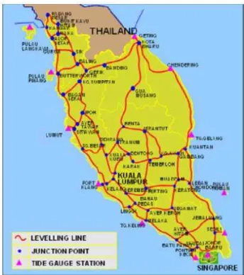
The first national geodetic vertical datum officially established in Malaysia was known as the Land Survey Datum 1912 (LSD12). The LSD12 was derived based on the observation of Mean Sea Level (MSL) for 8 months from September 1st, 1911 to May 31st, 1912 at Port Kelang (Jamil, 2011; Sulaiman, 2016). Until 1994, the LSD12 has remained unchanged since it was established in 1912. In 1983, DSMM began to re-determine the precise MSL value in conjunction with the establishment of the new Precise Levelling Network for Peninsular Malaysia as shown in Figure 4. This was carried out by the setting-up of a Tidal Observation Network that consists of 12 tide gauge stations. Subsequently, Port Kelang was chosen for the adoption as a reference level for the PMGVD origin, based on upon a 10-year tidal observation (from 1984 to 1993). The new MSL adopted is 3.624m above zero tide gauge. It was identified that PMGVD is lower than LSD by 65mm. The new MSL height was transferred from Port Klang using precise levelling to a Height Monument in Kuala Lumpur by 3 different precise levelling routes (Country Report, 2012; Sulaiman, 2016).

Figure 4. Precise Levelling Network (Country Report, 2012)

2. RESEARCH APPROACH

2.1 Quantification of Sea Level Rise Rate and Magnitude from Tidal Data

The tidal data used in this study was taken from Permanent Service for Mean Sea Level (PSMSL) with monthly averaged data. 12 tide gauge stations in Peninsular Malaysia are involved. The period of the data starts from January 1984 up to December 2015. The robust fit regression analysis is used to estimate the rate of sea level rise at tide gauge station. Then, the magnitude of sea level rise from the tidal data is quantified by subtracting mean of yearly in 2015 with mean of yearly in 1984 (it depends on the date of tide gauge establishment)..

2.2Quantification of Sea Level Rise Rate and Magnitude from Satellite Altimeter

For this study, the sea level from satellite altimeter is referred to the Mean Sea Surface (MSS) height, thus creating sea level anomaly. The most recent DTU13 MSS model released by Denmark Technical University is used as a datum to derive the sea level anomaly in this study. Multi-mission satellite altimetry data from TOPEX, Jason-1, Jason-2, ERS-1, ERS-2, EnviSat, CryoSat-2 and Saral/Altika are used to retrieve the daily sea level anomaly. The altimetry sea level anomaly data extracted

ranges between 1°N ≤ Latitude ≤ 8°N and 99°E ≤ Longitude ≤

Figure 5.Overview of altimetry data processing Flow in RADS

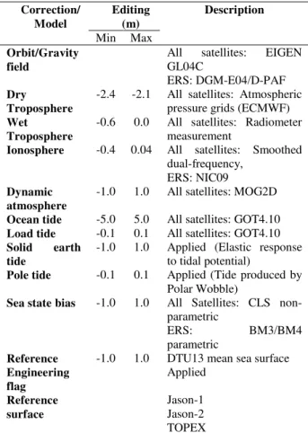
The sea level data are corrected for orbital altitude; altimeter range corrected for instrument, sea state bias, ionospheric delay, dry and wet tropospheric corrections, solid earth and ocean tides, ocean tide loading, pole tide electromagnetic bias and inverse barometer corrections. The bias is reduced by applying specific models for each satellite altimeter mission in RADS as shown in Table 1. After applying altimeter corrections and removing bias in RADS processing, the next step is to perform crossover adjustments.

Due to factors such as orbital errors and inconsistency of the satellite’s orbit frame, the sea surface heights (SSH) from different satellite missions need to be adjusted to a “standard” surface. Since the quality of the radial accuracy of the orbits and measurements of the TOPEX-class satellites (TOPEX, Jason-1 and Jason-2) surpasses the accuracy of the orbits and measurements of the ERS-class satellites (ERS-1, ERS-2, EnviSat, Cryosat-2 and Saral/ Altika), the so-called dual-crossover minimisation analysis was performed in this study (Schrama, 1989). The minimisation was achieved with the orbit of the TOPEX-class satellites held fixed and those of the ERS -class satellites adjusted concurrently (Trisirisatayawong et al, 2011).

In this case, only crossovers minimisation analysis between ERS-class and TOPEX-class satellites are considered. The area for the crossover minimisation is much larger than the area under investigation in order to have sufficient crossover information to estimate the smoothness (one cycle per orbital

revolution) of orbit error function fitting. The time frame

covered by individual crossovers is limited to 18 days to reduce the risk of eliminating real oceanic signal and, with that, sea level trend (Trisirisatayawong et al., 2011).

A distance-weighted gridding was applied in order to lose as little information as possible while still obtaining meaningful values for grid points located between tracks. In other words, the use of weighting function is to establish the points close to the centre to be important and points far from the centre to be relatively insignificant. The weighting function is based on Gaussian distribution, Fw(r) (Singh et al., 2004):

Fw(r) = (2)

Where, the sigma, represents the weight assigned to a value at a normal point located at a distance r from the grid point.

Table 1. Corrections and models applied for RADS altimeter processing.

Correction/ Model

Editing (m)

Description

Min Max Orbit/Gravity

field

All satellites: EIGEN GL04C

ERS: DGM-E04/D-PAF Dry

Troposphere

-2.4 -2.1 All satellites: Atmospheric pressure grids (ECMWF) Wet

Troposphere

-0.6 0.0 All satellites: Radiometer measurement

Ionosphere -0.4 0.04 All satellites: Smoothed dual-frequency,

ERS: NIC09 Dynamic

atmosphere

-1.0 1.0 All satellites: MOG2D

Ocean tide -5.0 5.0 All satellites: GOT4.10 Load tide -0.1 0.1 All satellites: GOT4.10 Solid earth

tide

-1.0 1.0 Applied (Elastic response to tidal potential)

Pole tide -0.1 0.1 Applied (Tide produced by Polar Wobble)

Sea state bias -1.0 1.0 All Satellites: CLS non-parametric

ERS: BM3/BM4 parametric

Reference -1.0 1.0 DTU13 mean sea surface Engineering

flag

Applied

Reference surface

Jason-1 Jason-2 TOPEX

The daily altimetry data from TOPEX-class and ERS-class are then filtered and gridded to sea level anomaly bins (0.25° by 0.25°) using Gaussian weighting function with sigma 2.0. Both temporal and spatial weighting on sea level anomaly is considered in the gridding step by choosing a square mesh with a block size of 0.25° (spatial) and cut-off at 18 days (temporal). This selection was performed based on the ERS-class type characteristics where the average track spacing is 0.72° and the repeat period is 35 days. This is to assure focus on altimetry data in the vicinity of mesh points (gridding block), but also allows for occasional data gaps. Subsequently, the daily solutions for sea level anomaly are combined into monthly average solutions. This technique aims to (more or less)

equalise the final monthly altimeter solution with the monthly

tide gauge solution as the satellite altimeter flies over the tide gauge only three times in a month (TOPEX-class) for the best case scenario, and in the worst case scenario only once a month (ERS-class). Hence, it gives rise to more fluctuations in the altimeter technique when compared to the tide gauge. It seems that the methodology undertaken (daily to monthly altimeter solution) improves the correlation between monthly solutions of altimetry and tidal data in this study (Din et al., 2015).

2.3 Quantification of Sea Level Rise Rate using Robust Fit Regression

The time series of the sea level trend in this study was quantified using robust fit regression analysis. Robust fit analysis is a standard statistical technique that concurrently deals with solution determination and outliers detection. In this

time series of each station in an Iteratively Re-weighted Least Squares (IRLS) technique. Depending on the deviations from the trend line, weights of measurements are adjusted accordingly. The trend line is then re-fitted. The process is repeated until the solution converges. The weights of the observations (wi) are readjusted by the adopted bi-square weight

function, whose relationship with normalised residuals, (ui) can

be written as (Holland and Welsch, 1977; Din et al., 2015):

wi = (3)

Where,

ui =

ri: Residuals, hi: Leverage,

S: Mean absolute deviation divided by a factor 0.6745 to make it an unbiased estimator of standard deviation

K: A tuning constant whose default value of 4.685 provides for

95% asymptotic efficiency as the ordinary least squares

assuming Gaussian distribution.

Observations that are assigned zero weights in any iteration are declared as outliers and eliminated from further computation (Holland and Welsch, 1977)

3. RESULTS AND DISCUSSION

3.1 Sea Level Rise Acceleration from Tide Gauge

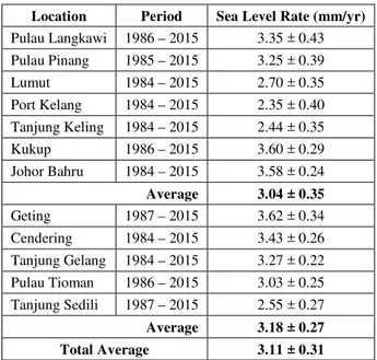
Table 2 gives the sea level rate from 1984 to 2015 (32 years) for all tide gauge stations in Peninsular Malaysia. At the west coast of Peninsular Malaysia, Kukup with 3.60 ±0.29 mm/yr experienced the highest sea level rate by robust fit regression. Meanwhile, Port Kelang experienced the lowest rate at 2.35 ±0.40 mm/yr by robust fit regression. The range of sea level rate by robust fit regression is from 2.35 ±0.40 mm/yr to 3.60 ±0.29 mm/yr. The average relative sea level rate for the west coast of Peninsular Malaysia calculated by robust fit regression yielded 3.04 ±0.35 mm/yr.

Table 2. Sea Level Rate (mm/yr) using Robust Fit Regression Analysis for All Peninsular Malaysia Tide Gauge Stations

For the east coast of Peninsular Malaysia, Geting with 3.62 ±0.34 mm/yr experienced the highest sea level rate by robust fit regression. On the other hand, Tanjung Sedili experienced the lowest rate at 2.55 ±0.27 mm/yr by robust fit regression. The range of relative sea level rate by robust fit regression for the east coast of Peninsular Malaysia is from 2.55 ±0.27 mm/yr to 3.62 ±0.34 mm/yr. For the west coast of Peninsular Malaysia, the average relative sea level rate calculated by robust fit regression yielded 3.18 ±0.27 mm/yr. By combining the relative sea level rate for both east and west coasts of Peninsular Malaysia, the average sea level rate calculated by robust fit regression was estimated at 3.11 ±0.31 mm/yr.

Figure 6 illustrates the example of the sea level trend at Pulau Pinang and Port Kelang determined using robust fit regression analysis. At Pulau Pinang tide gauge station, the estimated tidal sea level rate over between 1985 – 2015 (32 years) was 3.25 ±0.39 mm/yr. Also, the estimated rate at Port Kelang within thesame time period was 2.35 ±0.40 mm/yr.

Figure 6. Tidal Sea Level Rate Between 1984 – 2015 using Robust Fit Regression Analysis

3.2Sea Level Rise Magnitude from Tide Gauge

3.2.1 Tidal Yearly Magnitude from 1984 to 2015: The magnitude of sea level rise from tide gauge data at stations along the coast of Peninsular Malaysia was computed from the difference between the yearly mean of tidal data obtained in 2015 and that of 1984 or the year of tide gauge establishment. The outcome revealed that the smallest magnitude of -0.001m occurred at Tanjung Keling, while the largest magnitude of 0.092m occurred at Cendering. From the findings, the computed magnitude of sea level rise is clearly influenced by the “very strong” El Niño in 2015/2016 (ONI, 2016). This has more effect on tide gauge stations located along the Malacca Straits due to the fact that it is located in a semi-closed area and it also prevents the short term circulation dynamics from averaging out over this area which causes the mean sea level to have a disturbed annual cycle with lots of higher harmonics (Din et al.,

2012). It is interesting to note that Pulau Langkawi and Geting had the same magnitude of 0.074m. These estimates show that the magnitude of the sea level rise is inconsistent along the coast of Peninsular Malaysia. Table 3 shows details of the computed magnitude across all tide gauges used for this study. Location Period Sea Level Rate (mm/yr)

Table 3. Sea Level Rise Magnitude using Tidal Data (32 Years).

*Johor Bahru Tide Gauge was stopped the operational in 2014

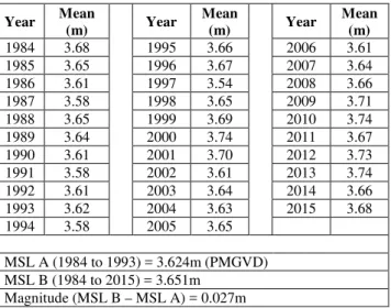
3.2.2 Tidal Average of 32 Years (1984 – 2015) Difference Tidal Average of 10 Years (1984 – 1993) for PMGVD

The computation was done using tidal data from Port Kelang tide gauge station in Peninsular Malaysia. Table 4 shows the yearly tidal average from 1984 to 2015. The difference between MSL from 10 years of tidal data (1984 – 1993) and that from 32 years (1984 – 2015) was computed for this station. The computed MSL B (3.651m) from data spanning 1984 – 2015 (32 years) shows the MSL is increasing towards the terrain, while the magnitude shows that the size of the movement of MSL B from MSL A is 27mm. Hence, the magnitude showed the long-term effect a change in MSL has on the Peninsular Malaysia geodetic vertical datum since Port Kelang is the adopted local vertical datum origin for Peninsular Malaysia.

Year Mean

(m) Year

Mean

(m) Year

Mean (m)

1984 3.68 1995 3.66 2006 3.61

1985 3.65 1996 3.67 2007 3.64

1986 3.61 1997 3.54 2008 3.66

1987 3.58 1998 3.65 2009 3.71

1988 3.65 1999 3.69 2010 3.74

1989 3.64 2000 3.74 2011 3.67

1990 3.61 2001 3.70 2012 3.73

1991 3.58 2002 3.61 2013 3.74

1992 3.61 2003 3.64 2014 3.66

1993 3.62 2004 3.63 2015 3.68

1994 3.58 2005 3.65

MSL A (1984 to 1993) = 3.624m (PMGVD) MSL B (1984 to 2015) = 3.651m

Magnitude (MSL B – MSL A) = 0.027m

Table 4. Yearly MSL at Port Kelang (1984 – 2015)

3.3 Sea Level Variation from Satellite Altimeter from 1993 to 2015

Sea level measured by satellite altimeter is relative to a global datum, known as absolute sea level. Satellite altimeter measures the absolute sea level relative to the standard ellipsoid (WGS84 ellipsoid), the most commonly used datum at present. Thus, satellite altimeters provide improved measurements of global sea level change due to their truly global coverage and direct tie to the earth's centre of mass (Fu and Cazenave, 2001). In this study, the sea level from satellite altimeter is referred to the Mean Sea Surface (MSS) height, thus creating sea level anomaly. The most recent DTU13 MSS model released by Denmark Technical University is used as a datum to derive the sea level anomaly in this study.

By using a similar method with relative sea level rate analysis, the absolute sea level rate is quantified using robust fit regression analysis in MATLAB. The altimetry data time frame begins from January 1993 up to December 2015 (23 years). To interpret the absolute sea level trend by mapping of the Malaysian seas, i.e., Malacca Straits and South China Sea, a numbers of altimeter-derived sea level anomaly points are extracted. The altimeter extracted points are focused for offshore or deep ocean areas because the residual of sea level anomaly increases closer to the coast due to the increased sea level variability in shallow water depth (Andersen and Scharroo, 2011).

Figure 7 demonstrates the absolute sea level rise rate over Malacca Straits and South China Sea. According to Figure 7, the results clearly show that the absolute sea level rise rate is rising and varying from place to place over the Peninsular Malaysian seas. The rate of sea level varies and gradually increases from west to east of Peninsular Malaysia. The Malacca Straits, the connection between the Andaman Sea in the Indian Ocean and the Sunda Shelf, has lower rate of absolute sea level rise trend compared to South China Sea. It ranges from 1.26 +/- 0.57 mm/yr to 4.39 +/- 0.60 mm/yr, and with an average of 3.14 +/- 0.12 mm/yr. This may due to the fact that the depth and shape of the Malacca Straits is shallow and rather narrow. Besides, the tides or water flows mainly enters from one side of the strait and are influenced by the geometrical changes from the north-west to south-east and the tiny islands at the south-east end (Akdag, 1996). Meanwhile, the absolute sea level rise in the South China Sea, which has a typical marginal sea characterised with a deep basin, shelf break, and shallow shelf, occurs at a rate of 3.22 +/- 0.32 mm/yr to 4.32 +/- 0.37 mm/yr. The average of the absolute sea level rise rate in the South China Sea is estimated at 3.85 +/- 0.05 mm/yr.

Yearly the sea level continues to rise due to global warming and other factors. In order to quantify the magnitude of sea level rise, the yearly sea level anomaly for 1993 and 2015 were plotted as shown in Figure 8. In 1993, the value of yearly sea level anomaly is at range of -7cm to 8 cm over Malacca Straits and South China Sea. The sea level anomaly magnitude in Malacca Straits is higher than South China Sea. The yearly sea level anomaly in 2015 is about -7cm to 9cm over both areas. From the results in Figure 8, yearly sea level anomaly in 2015 was subtracted with yearly sea level anomaly in 1993 to quantify the sea level rise magnitude. Refer to Figure 8; the magnitude of sea level rise is higher in South China Sea compared to Malacca Straits. The sea level rise magnitude is at range of 4cm to 10cm for South China Sea and -15cm to 6cm for Malacca Straits, respectively. Interestingly, results from the Location Time Range

Yearly Mean Sea Level Value (m)

Magnitude of SLR (m)

Cendering 1985 – 2015 2.187 – 2.279 0.092 Kukup 1986 – 2015 3.987 – 4.073 0.086 Pulau

Langkawi

1986 – 2015 2.182 – 2.256 0.074

Geting 1987 – 2015 2.252 – 2.326 0.074 Johor

Bahru*

1984 – 2013 2.852 – 2.915 0.063

Pulau Pinang

1986 – 2015 2.658 – 2.716 0.058

Pulau Tioman

1986 – 2015 2.812 – 2.866 0.053

Tanjung Gelang

1984 – 2015 2.804 – 2.840 0.035

Tanjung Sedili

1987 – 2015 2.373 – 2.400 0.028

Lumut 1985 – 2015 2.206 – 2.224 0.017 Port

Kelang

1984 – 2015 3.678 – 3.680 0.002

Tanjung Keling

1985 – 2015 2.868 – 2.866 -0.001

Minimum -0.001 Maximum 0.092

Figure 9 showed that most of the areas have a positive trend. It proves that there is a sea level rise over Malacca Straits and South China Sea, and the magnitude of sea level rise varies from place to place. Besides, the computed magnitude of sea level is clearly influenced by the “very strong” El Niño for the region in 2015/2016 (ONI, 2016).

Figure 7. Map of sea level rise rate over Malacca Straits and South China Sea. The rate is computed from 23 years of altimetry data ranging from 1993 to 2015. Units are in mm/yr.

Figure 8. Map of yearly sea level anomaly over Malacca Straits and South China Sea for year 1993 (Up) and year 2015 (Down). Units are in cm.

Figure 9. Map of sea level rise magnitude over Malacca Straits and South China Sea. The magnitude is computed from 23 years of altimetry data ranging from 1993 to 2015. Units are in cm.

3.4Discussion on Mean Sea Level (MSL) Simulation on Benchmark

Figure 10. MSL Height Variation at Port Kelang Benchmark

The height of the tide gauge bench mark B0169 was fixed relative to the MSL from the Port Kelang tide gauge zero. A long-term change in the MSL will result in a change in the geodetic vertical datum at the Bench mark. To verify the magnitude of this MSL change, old MSL (3.864m) at B0169 spanning 1984 – 1993 was compared to a new MSL (3.837m) spanning 1984 – 2015 tidal data. The resultant difference of -0.027m indicates the upward movement of the MSL closer to the terrain. Figure 10 gives a clearer illustration.

4. CONCLUSION

a change in MSL has on the geodetic vertical datum of Port Kelang tide gauge station. The findings are expected to be valuable particularly for a new insight on the establishment of national geodetic vertical datum based on mean sea level data.

ACKNOWLEDGEMENTS

The authors would like to thank to TU Delft, NOAA, Altimetrics Llc and the Permanent Service for Mean Sea Level (PSMSL) for providing altimetry and tidal data, respectively. We are grateful to the Ministry of Higher Education (MOHE) for funding this project under the FRGS Fund, Vote Number R.J130000.7827.4F706.

REFERENCES

Akdag, C. (1996). Tidal Analysis of the South China Sea. Technical Report; Delft Hydraulics. Group of Fluid Mechanics, Faculty of Civil Engineering, Delft University of Technology.

Andersen, O. B. and Scharroo, R. (2011). Range and Geophysical Corrections in Coastal Regions: And Implications

for Mean Sea Surface Determination. In Coastal Altimetry.

Springer. doi:10.1007/978-3-642-12796-0.

AVISO (2016). AVISO Satellite Altimetry Data. Retrieved July 25, 2016, from http://www.aviso.oceanobs.com/

Country Reports (2012). Nineteenth United Nations Regional

Cartographic Conference for Asia and the Pacific. Bangkok, 29

October – 1 November 2012 Item 6(a) of the provisional agenda. Conference papers.

Din, A. H. M., Omar, K. M., Naeije, M. and Ses, S. (2012).

Long-term Sea Level Change in the Malaysian Seas from

Multi-mission Altimetry Data. International Journal of Physical

Sciences Vol. 7(10), pp. 1694 - 1712, 2 March, 2012. DOI: 10.5897/IJPS11.1596.

Din, A. H. M., Reba, M. N. M., Omar, K. M., Pa’suya, M. F. and Ses, S. (2015). Sea Level Rise Quantification Using

Multi-Mission Satellite Altimeter over Malaysian Seas. The 36th

Asian Conference on Remote Sensing (ACRS 2015). October, 19 to 23, 2015. Manila, Philippines. Scopus - Proceeding.

DSMM (2012). Department of Surveying and Mapping

Malaysia. Retrieved June 01, 2012, from

http://www.geodesi.jupem.gov.my/

Fu, L. L. and Cazenave, A. (2001). Altimetry and Earth Science,

A Handbook of Techniques and Applications. Vol. 69 of

International Geophysics Series. Academic Press, London.

Holland, P. W. and Welsch, R. E. (1977). Robust Regression

using Iteratively Reweighted Least-squares. Communications in

Statistics—Theory and Methods 6 (9), 813–827.

Horton, R., Herdomjer, C., Rosenweig, C., Liu, J., Gornitz, V. and Ruane, A. (2008). Sea Level Projections for Current Generation CGCMs based on semi-empirical method.

Geophysical Research Letters, 35, L02715

Intergovernmental Panel on Climate Change (IPCC). (2007). Fourth Assessment Report Working Group I Report (WGI):

Climate Change 2007: The Physical Science Basis. Cambridge:

Cambridge University Press.

Jamil, H. (2011). GNSS Heighting and Its Potential Use in Malaysia. In GNSS Processing and Anallysis. Maarakehm Morocco: FIG Working Week 2011.

Meehl, G. A., Stocker, T. F., Collins, W. D., Friedlingstein, P., Gaye, A. T., Gregory, J. M., Kitoh, A., Knutti, R., Murphy, J. M., Noda, A., Raper, S. C. B., Watterson, I. G., Weaver, A. J., Zhao, Z.-C. in: Solomon, S., Qin, D., Manning, M., Chen, Z., Marquis, M., Averyt, K. B., Tignor, M. and Miller, H. L. (2007). Climate Change 2007: The Physical Sciences Basis. Contribution of Working Group 1 to the Fourth Assessment of the Intergovermental Panel on Climate Change, Cambridge University Press, Cambridge, UK and New York, NY, USA. pp. 747 – 845.

Mohamed, A. (2003). An Investigation of the Vertical Control Network of Peninsular Malaysia using a Combination of

Levelling, Gravity, GPS and Tidal Data. Doctor Philosophy,

Universiti Teknologi Malaysia, Skudai.

Naeije, M., Scharroo, R., Doornbos, E. and Schrama, E. (2008).

Global Altimetry Sea Level Service: GLASS. NIVR/SRON GO

project: GO 52320 DEO.

Nicholls, R. J. and Tol, R. S. J. (2006). Impacts and Responses to Sea-level Rise: a Global Analysis of the SRES Scenarios over

the Twenty-first Century. Philosophical Transactions of the

Royal Society A: Mathematical, Physical and Engineering Sciences, 364 (1841), 1073-1095.

ONI (2016). The Oceanic Niño Index. Retrieved July 30, 2016, from http://ggweather.com/enso/oni.htm.

Pittock, A. B. (2009). Climate Change: The Science, Impacts

and Solutions. 2nd edition. Collingwood, VIC. CSIRO

Publishing.

PSMSL (2016). Permanent Service for Mean Sea Level. Retrieved July 28, 2016, from http://www.psmsl.org/

Schaeffer, M., Hare, W., Rahmstorf, S. and Vermeer, M. (2012). Long-term sea-level rise implied by 1.5°C and 2° C

warming levels. Nature Climate Change Letters. Published

online: 24 June, 2012.

Schrama, E. (1989). The Role of Orbit Errors in Processing of

Satellite Altimeter Data. Netherlands Geodetic Commission,

Publication of Geodesy 33, 167 pp.

Singh, M., Mandal, M. and Basu, A. (2004). Robust KLT tracking with Gaussian and Laplacian of Gaussian weighting functions. Proceedings of the 2004 null: IEEE, 661-664.

Sensing and Spatial Information Sciences, Kyoto, Japan, Vol. XXVII, Part B1, pp. 456-469.

Solomon, S., Qin, D., Manning, M., Chen, Z., Marquis, M., Averyt, K. B., Tignor, M. and Miller, H. L. (Eds.) (2007).

Climate change 2007: The physical science basis. In

Sulaiman, S. A. (2016). Gravimetric Geoid Model Determination for Peninsular Malaysia using Least Squares

Modification of Stokes. Doctor Philosophy, Universiti

Teknologi Mara (UiTM), Shah Alam.

Trisirisatayawong, I., Naeije, M., Simons, W. and Fenoglio-Marc, L. (2011). Sea Level Change in the Gulf of Thailand from

GPS Corrected Tide Gauge Data and Multi-Satellite Altimetry.

Global Planetary Change, 76: 137-151.

Vermeer, M. and Rahmstorf, S. (2009). Global sea level linked

to global temperature. Proceedings of the National Academy of

Sciences of the United States of America (PNAS), 106 (51), 21527-21532.

Watson, C. S. (2005). Satellite Altimeter Calibration and

Validation using GPS Buoy Technology. Doctor Philosophy,

Centre for Spatial Information Science, University of Tasmania, Australia, 264pp. Available at: http://eprints.utas.edu.au/254/

Woodard, G., Perkins, D. and Brown, L. (2010). Climate change and freshwater ecosystems: impacts across multiple

levels of organization. Philos Trans R Soc Lond B Biol Sci.,