Sergio Rodrigo Vale**
Summary: 1. Introduction; 2. Econometric methodology; 3. Data; 4. Empirical results; 5. Conclusion.
Keywords: Inflation; growth; uncertainty; bivariate GARCH-in-mean.
JEL codes: C32; E20; E31.
In this paper I intend to estimate a bivariate GARCH-in-Mean in order to test four hypotheses about Brazilian economy. First, I want to know whether inflation uncertainty has a positive impact on the level of inflation as predicted by Cukierman and Meltzer (1986). Second, I want to test if this uncertainty has a negative impact on growth as proposed by Friedman (1977). Third, it will be tested the hypothesis of a negative impact of uncertainty growth on the level of growth as pointed out by Ramey and Ramey (1991). Finally, I will test if this uncertainty has a positive impact on the level of inflation as predicted by Deveraux (1989). The findings are a little mixed but in all settings they corroborate Cukierman and Meltzer explanation and some of them corroborate Friedman’s theory.
O objetivo deste artigo e estimar um GARCH-in-Mean bivariado para testar quatro hip´oteses sobre a economia brasileira. Primeiro, quero testar se a incerteza inflacionaria tem um impacto positivo no n´ıvel de inflac˜ao como previsto por Cukierman and Meltzer (1986). Segundo, testo se esta incerteza tem um impacto negativo no cresci-mento como proposto por Friedman (1977). Terceiro, ser´a testada a hip´otese de um impacto negativo da incerteza no crescimento so-bre o n´ıvel de crescimento como apontado por Ramey and Ramey (1991). Finalmente, testarei se esta incerteza tem um impacto positivo no n´ıvel de infla¸c˜ao como previsto por Deveraux (1989). Os resultados s˜ao variados, mas em todos os modelos estimados corrobora-se a hip´otese de Cukierman e Meltzer e em alguns se corrobora a hip´otese de Friedman.
*This paper was received in Aug. 2002 and approved in Aug. 2004. I would like to thank
Kenneth West and an anonymous referee for useful remarks and CNPq for the financial support. All remaining errors are my sole responsibility.
1. Introduction
The relationship between inflation and growth has become an intense research branch since the Mundell-Tobin effect was first described. In this earlier formu-lation the connection between economic growth and inflation comes out from a framework that has only two assets: money and capital. In steady state an in-crease in the rate of return of money implies a dein-crease in return of the other asset (they are assumed to be substitutes in the household portfolios). In other words, an increase in inflation positively impacts capital accumulation and consequently growth.1 But this result has systematically been challenged in empirical and the-oretical papers. For instance, Jones and Manuelli (1995) and De Gregorio (1993) points out that inflation is a tax on capital in models with cash-in-advance require-ment for investrequire-ment and, as a consequence, impacts growth negatively. Similarly, most of empirical papers has shown a negative relationship between these two variables but without a theoretical agreement about the reasons for the negative relation.2 But in economies with high uncertainty in growth and inflation the simple relationship between those two variables may be unsatisfactory.
With this explanation gap in mind, Friedman’s Nobel lecture pointed out an-other type of interference on growth. His argument hinges on two mechanisms. First, changes in the optimal wage contract length and the degree of wage in-dexation caused by inflation uncertainty could increase unemployment and, by some sort of Okun‘s Law, decrease growth. Second, increased volatility in infla-tion causes a less efficient system for coordinating economic activity. Based in arguments stemmed from Hayek (1945) and Lucas (1973), he argues that stable prices and stable price changes ease the signal extraction of relative prices from the observed absolute prices. Thus, when general inflation is more uncertain it is more difficult to extract relative prices from absolute prices. At the end of the process, absolute prices become innocuous and the agents resort to an alternative currency or to barter. This was the Brazilian case between mid-eighties and mid-nineties when we went through a hyperinflation process and currency lost practically all its value.3
1See Walsh (1998) for a survey of the models used to explain this relation.
2For instance, Bruno and Easterday (1998) show that high inflation economies are more
sus-ceptible to find negative relations between growth and inflation but that in cross-section analysis this relation seems to be ambiguous or even inexistent. The reason is that rapid and huge in-creases and dein-creases in inflation has a boom effect on growth which is not captured in mild inflationary processes. However, Barro (1996) uses another data set and find a negative cross-section relation between the two variables in fairly general contexts using arguments similar to Jones and Manuelli (1995).
Cukierman and Meltzer (1986) claim that increases in inflation uncertainty raise the optimal average inflation rate by increasing the incentive for the policy-maker to create inflation surprises. In their model Central Bank dislikes inflation but likes to stimulate economy. Ambiguity and lack of commitment over policies induce a higher variance of monetary growth and a higher variance in employment but agents cannot distinguish where this variance comes from. As a consequence the ambiguity allows the Central Bank to create inflation surprises.4 This seems also to be the case in Brazil where a Central Bank managed by the political con-venience of the moment prevented it to have a clear monetary policy.
Deveraux (1989) extended Barro and Gordon (1983) model to show that vari-ability in real shocks can positively affect inflation. The reason is that an ex-ogenous increase in the growth uncertainty lowers the optimal quantity of wage indexation. From the point of view of the policymaker a lower indexation can make surprise inflation more effective and, as a result, increase the average in-flation rate. Therefore, Devereux concludes that output growth uncertainty can increase inflation.
Finally, Ramey and Ramey (1991) suppose a simple general equilibrium model in which firms make technology commitments in advance, e.g., the determination of the scale of a new factory or the size of the attached labor force. Each technology corresponds to a different minimum efficient scale and in the absence of economic fluctuations firms would choose their technology to bring minimum efficient scale into line with the equilibrium output level. However, if growth volatility (higher economic instability) increases, equilibrium output levels may depart from mini-mum efficient scale and firms may end up with average costs above the minimini-mum level. Thus, volatility causes firms‘ production plans to be sub optimal ex-post and as a consequence growth uncertainty diminishes the average real growth.
What these apparently unrelated arguments have in common is the system-atic connection between uncertainty measures (in growth and inflation) and the respective level measures. To estimate these relations simultaneously I will apply
adversely affects long run growth but the effect can be quite the contrary in the short run. The reason for this positive relationship in the short term stems from a precautionary savings motive. But Issler et al. (1998) show that precautionary savings in Brazil is not significant.
4Ball (1992) proposes an inverse relationship. In his paper the causality runs from high
a bivariate GARCH-M model using output growth and inflation as the dependent variables in the mean equation. The right hand side will contain variables that help to forecast growth and inflation and the uncertainty measures, which are calculated from the equations errors.
Specifically, I intend to test four hypotheses for Brazilian economy. First, I want to know whether inflation uncertainty adversely impacts real growth, as predicted by Friedman; second, whether inflation uncertainty positively impacts inflation rate as pointed by Cukierman and Meltzer; third, whether growth uncer-tainty raises average inflation as shown in Devereux‘s model and, fourth, whether a more volatile growth promotes a lower average growth, as proposed by Ramey and Ramey.
The paper will be divided in five parts. Besides this introduction, the second part will quickly describe the bivariate GARCH methodology I will use. The third section will present the data used in this work. The fourth part will show the estimations made and, finally, the last part will conclude.
2. Econometric Methodology
We want to calculate the impact of uncertainty variables on level variables. The best way to do this is applying a bivariate GARCH-M model that has the following specification
πt=α0+α1xt+β1σ2s+β2σv2+ǫt (1)
yt=α2+α3zt+β3σ2s+β4σv2+vt (2)
Ht=C
′
C+
K
X
k=1
q
X
i=1
A′ikηt−1η
′
t−1Aik+
K
X
k=1
p
X
i=1
GikHt−iGik (3)
where t is the inflation rate, yt is the growth rate, xt and zt are explanatory
variables that help to forecast inflation and growth, σǫ2 andσv2 are the conditional variance of the error in the first and second equations, respectively. The third equation shows the variance-covariance process where C, Aik and Gik are n x n
parameter matrices withC triangular. K determines the generality of the process. This specification is called BEKK model and is due to Engle and Kroner (1995). Its improvement upon other models of this class is that the representation for the
we have less parameters to estimate compared to traditional Vec representations.5 This model also has a difference with traditional models because we add uncer-tainty measures in the mean equations. This representation stems from Bollerslev et al. (1988) but they calculate their model using a Vec representation. To avoid too many parameters to estimate we will suppose a GARCH-M (1,1) formulation where Ht is given by:
Ht=C′C+
·
a11 a12
a21 a22
¸′·
ǫ2t−1 ǫt−1vt−1
vt−1ǫt−1 vt2−1
¸ ·
a11 a12
a21 a22
¸
(4)
·
g11 g12
g21 g22
¸′
Ht−1
·
g11 g12
g21 g22
¸
Following the suggestions made by Grier and Perry (2000)’s paper, I will first estimate single equations by OLS for equations (1) and (2) without the uncertainty measures. With this I will test for equations (1) and (2) the presence of ARCH terms by a Ljung-Box test. The estimation method will be by quasi-maximum likelihood proposed by Bollerslev and Wooldridge (1992). Their estimator is con-sistent for nonnormality of the residuals, which is a common feature of this kind of model.6 Finally, the estimation of (1), (2) and (4) will follow the numerical optimization algorithm proposed by Berndt et al. (1974) and known as BHHH.
3. Data
I am using monthly Brazilian data to estimate the model. The series are season-ally adjusted industrial production7 and PPI both calculated by IBGE (Brazilian Institute of Geography and Statistics). Additionally, I will use CPI provided by FIPE (Institute of Economic Research Foundation).8 The reason to use a different source is that the CPI calculated by IBGE only started to run in 1979 and I intend to use a longer series. Moreover, PPI is not calculated by FIPE. For the inflation series we havet= log(Pt/Pt−1)∗100 wherePtis the price index for each series and
growth is given by yt= log(IP t/IPt−1)∗100 where IPt is the industrial
produc-tion index. In the growth equaproduc-tion I also use a default risk measure given by the
5See Bollerslev et al. (1994) and Engle and Kroner (1995) for more details.
6Grier and Perry’s paper uses the traditional maximum likelihood estimation for US data but
does not care about the nonnormality of the residuals.
7The reason for using industrial production instead of a general measure of GNP is that this
monthly data is only available from 1991 on.
8Alternative estimations using CPI calculated by FGV (IGP-DI) delivered similar results and
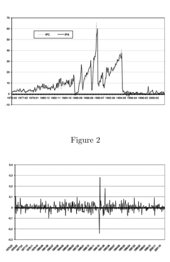
difference between the working capital interest rate and the overnight interest rate. The first series is a lending rate (Capital de Giro) and the second is a series that represents the most traded Treasury Note at the moment.9 The available range is from January 1975, when the industrial production index was first measured, to December 2001. We could estimate the same model using yearly data but the problem is that the range is too short to give accurate results since we depend on asymptotic results provided by the quasi-maximum likelihood estimation.10 The series used in this work are depicted in figures 1 and 2.
Figure 1
-10 0 10 20 30 40 50 60 70
1975:03 1977:02 1979:01 1980:12 1982:11 1984:10 1986:09 1988:08 1990:07 1992:06 1994:05 1996:04 1998:03 2000:02 IPC IPA
Figure 2
-0,3 -0,2 -0,1 0 0,1 0,2 0,3 0,4
1975:031976:021977:011977:121978:111979:101980:091981:081982:071983:061984:051985:041986:031987:021988:011988:121989:111990:101991:091992:081993:071994:061995:051996:041997:031998:021999:011999:122000:112001:10
9This occurs because some securities were changed due to changes of government or due to
a stabilization plan that launched a different Treasury Note. See Cenarios (no date) for more details.
10Nonnormality of residuals also was detected in a preliminary estimation of the model with
4. Empirical Results
4.1 Unit root tests for inflation and growth
The natural result when we test for unit root in growth and inflation is to find a stationary process for both series. In fact, when we apply the traditional ADF and PP (Philips-Perron) unit root tests we get two stationary series as a result. However, Perron et al. (1999) showed that this is not the case for the Brazilian inflation, where we had six stabilization plans in less than ten years. This occurs because ‘we can view the stabilization plans as creating ‘inliers’ whose magnitude is related to the current level of the series. Hence, if the series truly has a stochastic trend or even an explosive path, the magnitude of these inliers are, themselves, non-stationary random variables that have a tendency to increase as inflation increases. Since these shocks plans have failed, the series exhibits a tendency to return to its old (non-stationary) trend path after each episode. This is basically what contaminates the standard statistical measures, since the failures of the shock plans create a kind of spurious mean-reverting aspect to the series’ (Perron et al. (1999, p.28)). The data they used to test for unit root ended in June, 1993, months before the last stabilization plan (Real Plan) and the only one that knocked inflation down permanently. Thus, besides the inliers dummies for the flawed plans we have to add permanent break dummies due to the stabilization plan that worked (the Real Plan).11 The formulation for the ADF test based on the ‘innovational outlier‘ framework presented in their paper is given by:
yt = µ+γt+ p
X
j=1
(kjda(j)t+λjdb(j)t+φjD(j)t) +θ1DUt+θ2DUt (5)
+ θ3D(T B)t+αyt−1+
k
X
i=1
ci∆yt−i+ζt
where j correspond to each one of the five stabilization plans; da(j) = 1 in the first month of the plan and 0 otherwise (pulse dummy); db(j) = 1 for the first
11According to Perron in a previous change of e-mails this addition does not change the results
month after the end of the plan and 0 otherwise (pulse dummy); D(j) = 1 during the plan and 0 otherwise12 (level dummy). Additionally, we add three dummies related to the Real Plan: DUt = 1 if t > TB and 0 otherwise; DTt=t itt > T B
and 0 otherwise and D(T B)t= 1 if t=T B+ 1 and 0 otherwise. This equation is a mix of the equation (14) in Perron’s (1989) paper and equation (15) in Perron et al.’s (1999) paper.
An additive outlier model can also be formulated and it has the following expression:
yt=µ+γt+ k+1
X
i=0
p
X
j=1
φj,iD(j)t−i+θDTt+ϕDLt+αyt−1+
k
X
i=1
ci∆yt−i+ζt (6)
The results in table 1 and 2 are a little mixed with the innovational outlier model pointing to no unit root for PPI. But I will stick with the additive outlier model because the change in inflation process was abrupt and not gradual as supposed by the innovational outlier model. Moreover, the GARCH-M estimated without differencing PPI never presented invertible AR terms and delivered poor results. Thus, I will accept the null hypothesis of one unit root for both series.
Finally, the traditional ADF unit root test performed for the growth rate pointed out an ADF statistic of -10.52, which means that growth rate is sta-tionary at 1%. The same statistic for the default risk measure is -5.47 and it also means that this variable is stationary at 1%.
With these results the GARCH system will have a mean equation for the growth level and a mean equation for the first difference of the inflation rate. This is not really unconformable with our theories because they suppose that not only inflation rate can have the desired impacts we want but the growth rate of inflation too.13
12Perron and Vogelsang (1994) discuss the exact period of each plan and presents a table with
the duration of each plan.
13See particularly the discussion in Friedman (1977). In fact, he puts more influence of the
Table 1
Unit Root Test (ADF-Perron-Cati-Garcia innovational outlier model)
Series t-statistic αˆ lags
CPI -3.52** 0.861 1
PPI -6.21 0.763 1
Note: The decision rule was based on BIC criterion and the general-to-specific rule. Additionally, Ljung-Box tests were performed in the residuals and all showed white noise. ** de-notes one unit root at 5%. The critical value is based on Perron (1989) and de-pends on the break date. In our case we have to divide the number of ob-servations until the break divided by the total number of observations. This givesλ= 245/322≈0.8 and using
ta-ble VI.B in Perron for this value we get a critical value of -4.04 at 5%.
Table 2
Unit Root Test (ADF-Perron-Cati-Garcia additive outlier model)
Series t-statistic αˆ lags
CPI -1.28** 0.949 3
PPI -3.88 0.864 3
Note: The decision rule was based on BIC criterion and the general-to-specific rule. Additionally, Ljung-Box tests were performed in the residuals and all showed white noise. ** de-notes one unit root at 5%. The critical value is based on Perron (1989) and de-pends on the break date. In our case we have to divide the number of ob-servations until the break divided by the total number of observations. This givesλ= 245/322≈0.8 and using ta-ble VI.B in Perron for this value we get a critical value of -4.04 at 5%.
4.2 OLS models for inflation and growth
is fundamental for choosing the method of estimation. Second, the estimation of the single equations allows preliminary diagnose tests on the residuals in order to detect the presence of GARCH terms.
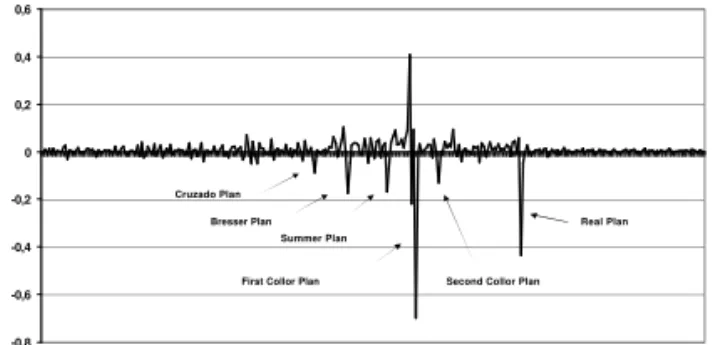
The results show the existence of correlation in the squared residuals in all equations, which is a signal of the presence of ARCH terms. Clearly, this does not mean that the existence of ARCH terms is guaranteed in the bivariate system but it will turn out to be true when I estimate the system. Note that we added dummies to each equation. These dummies have value 1 at the moment of the stabilization plan and zero otherwise and are named after the definition given before. The inclusion of these dummies occurs because when the inflation series are differentiated they show negative spikes due to the implementation of each stabilization plan as is shown in figure 3. Without the dummies the inflation equations presented pour results in terms of Schwartz criterion (SIC) and Ljung-Box test.14 Moreover, these dummies eliminate the spurious increase in volatility caused by the immediate afterwards of each economic plan.
It is interesting to note that the inclusion of the default risk rate turned out to be insignificant in the growth equation as well in the bivariate GARCH and thus will not be considered in the estimations. Note also that the Jarque-Bera test points out to the nonnormality of the residuals, which indeed indicate the necessity of using quasi-maximum likelihood methods.
An alternative modeling was tried. We estimated a VAR to capture bivariate relations between the growth and inflation mean equations.15 Using a sequential modified LR test and SIC criterions a VAR (3) was chosen using CPI16 However, in this case many of the estimated parameters were not significant and the mul-tivariate statistical tests were quite poor17 Similar results were found for PPI for
14It is necessary to note that we used SIC as the decision criterion for the most parsimonious
model throughout the paper. A multivariate version of SIC is used for the bivariate GARCH and it is detailed on the next section.
15It is well known that even if there are MA components in the system we can approximate a
VARMA by a VAR with a reasonable number of lags.
16The sequential modified LR tests as proposed by Lutkepohl (1991) is given by LR =
(T−m){log|Ωl−1| −log|Ωl|} −χ2¡K2¢ wheremis the number of parameters to be estimated in each equation and (T−m) is a small sample modification proposed by Sims (1980). Here we test that the coefficients on lag l are jointly zero using the 2 statistic. It is worthwhile to say that Atkins (AIC) and Hannan-Quinn (HQ) criterions also pointed 3 lags as the best model.
17For instance, a multivariate LM test such as the one proposed by Johansen (1995) points
which a VAR (3) was also identified. But since this is a preliminary view with the sole intention of identifying the presence of heteroskedasticity we must rely on our bivariate GARCH estimation to analyze if there is conditional volatility or not.
Table 3
OLS regressions for inflation and growth - 1975:03 to 2001:12
A: Growth
yt= 0.0001
(0.0001)−(00..3205)yt−1−(00.10
.05)ǫt−3+ 0(0.16
.05)ǫt−9
Log likelihood function = 1331.4 Ljung-BoxQ(4) = 6.82 (0.14) Ljung-BoxQ(12) = 20.03 (0.07) Ljung-BoxQ2(4) = 31.99 (0.00) Ljung-BoxQ2(12) = 46.74 (0.00) Jarque-Bera = 2946.7 (0.00)
B: CPI
πt= 9.06
(3.09)+ 0(0..2506)πt−1+ 0(0..7506)πt−3−(00..1605)πt−5+ 1(0..0207)vt−1 + 0.84
(0.08)vt−2−(00..2806)vt−4−(00..1506)vt−5+ 0(0..1104)vt−9−(13..4683)da(1) 5.70
−(1.83)da(2)−(13..6386)da(3) + 20(3..20)20da(4) + 5(1..2495)da(5)−16(2..00)20D(T B) Log likelihood function = -773.6
Ljung-BoxQ(4) = 6.23 (0.18) Ljung-BoxQ(12) = 10.04 (0.69) Ljung-BoxQ2(4) = 82.18 (0.00) Ljung-BoxQ2(12) = 83.32 (0.00) Jarque-Bera = 1894 (0.00)
C: PPI
πt= 9.48
(3.91)+ 1(0..2705)πt−1−(00.48
.09)πt−2−(00.18
.06)πt−3−(00.20
.06)vt−4
−(00.20
.06)vt−11−(11.72
.90)da(1)−(12..2989)da(2)−(17..3092)da(3) +16.65
(2.96)da(4) + 6(1..8193)da(5)−(11..2193)D(T B) Log likelihood function = -789.8
Ljung-BoxQ(4) = 4.39 (0.182) Ljung-BoxQ(12) = 10.89 (0.620) Ljung-BoxQ2(4) = 59.40 (0.000) Ljung-BoxQ2(12) = 80.64 (0.000) Jarque-Bera = 201.3 (0.00)
Note: standard errors are in parentheses under the coefficients.Q(4) andQ(12) are the Ljung-Box statistics for fourth- and twelfth-order serial correlation in the residuals. Q2(2) and Q2(12) are the same
statistics but it corresponds to the serial correlation in squared resid-uals. Jarque-Bera is the test for normality of residresid-uals. The numbers in parentheses after these statistics are the p-value. BIC was also used as a criterion for decision. The dummiesda(j) andD(T B) correspond
to the definition given before. The first one has 1 at the moment of the stabilization plan and zero otherwise in the first five plans and
D(T B) is 1 for the moment of implementation of the Real Plan and zero otherwise.
Figure 3
-0,8 -0,6 -0,4 -0,2 0 0,2 0,4 0,6
1975:031976:021977:011977:121978:111979:101980:091981:081982:071983:061984:051985:041986:031987:021988:011988:121989:111990:101991:091992:081993:071994:061995:051996:041997:031998:021999:011999:122000:112001:10
Cruzado Plan
Bresser Plan Summer Plan
First Collor Plan Second Collor Plan Real Plan
4.3 Bivariate GARCH(1,1)-M for inflation and growth and
discus-sion
The results presented in Tables 4 and 5 show that the estimated equations correct for the existence of GARCH terms in the residuals and this can be seen by the Ljung-Box test on the squared residuals. It is important to note that a multivariate SIC criterion was used to find the most parsimonious model and it is given by
SIC= ln
¯ ¯ ¯
¯d
X¯¯¯
¯+
lnn
n (number of freely estimated parameters)
18 (7)
wherenis the number of observations andPis the estimated variance-covariance matrix.
Additionally, a multivariate LM test for the residuals was performed. Following Doornik (1996) we test that LM =T nR2
m with aχ2(sn2) asymptotic distribution
whereT is the number of observations,nis the number of equations in the system and R2m is given by
R2m= 1−tr½³Vˆ′Vˆ´ ³V′
0V0
´−1¾
18We considerer Hannan-Quinn criterion as an alternative but it did not change the results.
where V are the residuals of the regressions supposing the residuals are auto correlated andV0are the residuals under the null hypothesis of no autocorrelation. Despite the L-B tests for the growth mean equations be a little disappointing it was the best specification found. Note that I used the conditional standard deviation instead of the variance in the mean equations because the system did not converge when I tried the conditional variance.
The variance-covariance estimates are formatted as presented in equation (4) and all coefficients are significant. When 0 appears instead of one of the coefficients it means that it was not significant and it was dropped of the equations.
In table 4, where I use CPI, the results show that two of the coefficients do not have the expected sign. In fact, only the inflation uncertainty measure (σv)
on the inflation equation and on the growth equation was significant and had the right sign. The growth uncertainty measure (σǫ) presented the wrong sign and
was not significant in both equations. This means that inflation uncertainty had a higher impact than growth uncertainty in this period on both variables. Indeed, inflation was the central economic problem throughout this period and economic agents had a major worry about the impacts of a huge and increasing inflation on growth and on inflation itself.
The results for PPI are a little different in terms of significance but present the same coefficients signs of CPI‘s results and similar magnitudes. Particularly, inflation uncertainty is still significant in the inflation equation but it is not in the growth equation. And nowσǫhas a significant and positive impact on the growth
equation, which contradicts Ramey and Ramey theoretical findings. It should be natural to stick with the alternative interpretation given by Black (1987), which proposes a positive relationship between these two measures based on the impacts of a high-risk technology on the output growth in a business cycle framework. But we can raise other issues to this empirical finding. In fact, following an argument by Varian (1992, p.43), suppose that a firm faces fluctuating prices for its output. Suppose that the firm gets p1 with probabilityq and p2 with probability (1−q). The average price for this firm is ¯p = qp1+ (1−q)p2. Now, let’s compare the profits when the price fluctuates to the profits at the average price. Since the profit function is convex, we get
qπ(p1) + (1−q)π(p2)≥π(qp1+ (1−q)p2) =π(¯p)
is worthwhile to say that in a similar calculation made with US data Grier and Perry (2000) results accepted only Friedman’s hypothesis in all the samples they estimated.
An estimation considering a VAR(3) as identified in the last section also was applied. However, the multivariate SIC pointed out to our model as the best one instead of the VAR(3) for both CPI and PPI.
Table 4
Bivariate GARCH : CPI and Growth - 1975:3 to 2001:12
πt= 0.15
(0.06)−(00..4206)vt−1−(00.21
.058)vt−2+ 0(0.07
.02)vt−9−(19.44
.08)da(1)−14(7..83)23da(2)
−15.34
(1.31)da(3)−24(5..13)57da(4)−(25..8519)da(5)−35(3..25)97D(T B)−(00..9062)σǫt+ 0(0..1605)σvt
yt= 0.005
(0.12)−(00..3504)yt−1+ 0(0.18
.06)ǫt−1+ 0(0.15
.06)ǫt−9+ 0(0.36
.40)σǫt−(00..0505)σvt · σ2 y,t 0 σ2 πy,t σ 2 π,t ¸ =
(00..1002) 0
−0.12 (0.11) (00..3908)
(00..1002) −(00..1211) 0 0.39
(0.08) +
(00..3405) −(00..007004) 0 0.84
(0.06)
· vt2−1 ǫt−1vt−1 vt−1ǫt−1 ǫ
2
t−1
¸
(00..3405) 0 0.007 (0.004) (00..8406)
+
(00..8903) 0 0 0.66
(0.04)
· σπ,t2 −1 σ
2
πy,t−1 σ2
πy,t−1 σ
2
y,t−1
¸
(00..8903) 0 0 0.66
(0.04)
Residual Diagnostics Tests CPI Growth Ljung-Box Q(12) 18.00(0.054) 13.75(0.18) Ljung-Box Q(24) 30.12(0.12) 56.33(0.00) Ljung-Box Q2(12) 6.28(0.79) 18.46(0.04) Ljung-Box Q2(24) 14.71(0.87) 29.86(0.12) LM test = 3.84
Note: πt is the first difference of the inflation rate, yt is the growth rate
of industrial production,da(1) toda(5) are dummies for the first five eco-nomic plans with value 1 in the moment of implementation of the stabiliza-tion plan and zero otherwise, d(T B) is the same thing for the Real Plan (these dummies are better specified in the text). The values in parentheses for the diagnose tests are p-values. Standard errors are calculated using the consistent variance-covariance matrix proposed by Bollerslev and Wooldridge (1992). The residuals are standardized, i.e., we make all analysis based on
ǫt/σt whereσtis the conditional variance. LM test is estimated as specified
Table 5
Bivariate GARCH : PPI and Growth - 1975:3 to 2001:12
πt= 0.05
(0.15)+ 0(0..6812)πt−1−(00.18
.08)πt−2−(01.08
.13)vt−1+ 0(0.32
.12)vt−2−(18.76
.73)da(1)
−7.46
(3.40)da(2)−(17..3500)da(3)−(36..7616)da(4)−(15..2267)da(5)−18(2..80)11D(T B)−(00..5456)σǫt+ 0(0..0903)σvt
yt=−0.07
(0.06)−(00..3105)yt−1+ 0(0.14
.04)ǫt−3+ 0(0.27
.03)ǫt−9+ 0(0.43
.16)σǫt−(00..006008)σvt · σ2 y,t 0 σ2 πy,t σ 2 π,t ¸ =
(00..2401) 0
−0.14 (0.12) (00..3111)
(00..2401) −(00..1412) 0 0.31
(0.11) +
(00..7505) −(00..7237) 0 0.57
(0.06) ·
v2
t−1 ǫt−1vt−1 vt−1ǫt−1 ǫ
2
t−1
¸ −
0.75 (0.05) 0
−0.72
(0.37) (00..5706) +
(00..1016) 0 0 0.84
(0.02) ·
σ2
π,t−1 σ
2
πy,t−1 σ2
πy,t−1 σ
2
y,t−1
¸
(00..1016) 0 0 0.84
(0.02)
Residual Diagnostics Tests CPI Growth Ljung-BoxQ(12) 5.61(0.77) 16.88(0.07)
Ljung-BoxQ(24) 13.92(0.87) 66.36(0.00) Ljung-BoxQ2(12) 6.78(0.65) 9.53(0.48) Ljung-BoxQ2(24) 11.91(0.94) 21.82(0.47) LM test = 2.01
Note:πtis the first difference of the inflation rate,ytis the growth rate of industrial production,da(1) toda(5) are dummies for the first five economic plans with value 1 in the moment of implementation of the stabilization plan and zero otherwise,d(T B) is the same thing for the Real Plan (these dummies are better specified in the text). The values in parentheses for the diagnose tests are p-values. Standard errors are calculated using the consistent variance-covariance matrix proposed by Bollerslev and Wooldridge (1992). The residuals are standardized, i.e., we make all analysis based onǫt/σt where σt is the conditional variance. LM test is estimated as specified in
the text. The iterative method used was BHHH and the estimations were made in RATS 4.2.
5. Conclusion
that growth uncertainty should increase inflation and, finally, Ramey and Ramey proposed a negative connection between growth uncertainty and growth. Only Cukierman and Meltzer‘s hypothesis was accepted for all the estimations.
Some of the other theories were not rejected in the estimations. Indeed, when using CPI as the inflation measure we found a significant negative connection between inflation uncertainty and growth and when using PPI we found a result that contradicts Ramey and Ramey and for which there are few alternative and plausible explanations as far as I know.19
Besides new theoretical research we could estimate a Markov switching model where Brazil goes from stability to explosive growth in prices and then back again. But this will be done in another paper.20
References
Ball, L. (1992). Why does high inflation raise inflation uncertainty? Journal of Monetary Economics, 29:371–388.
Barro, R. J. (1996). Inflation and growth. Federal Reserve Bank of St. Louis Review, 78(3):450–467.
Barro, R. J. & Gordon, D. B. (1983). Rules, discretion and reputation in a model of monetary policy. Journal of Monetary Economics, 12:101–121.
Berndt, E., Hall, B., Hall, R., & Hausman, J. (1974). Estimation and inference in nonlinear structural models. Annals of Economic and Social Measurement, 3:653–665.
Black, F. (1987). Business Cycle and Equilibrium. Basil Blackwell, New York.
Bollerslev, T., Engle, R., & Nelson, D. (1994). ARCH models. In Engle, R. F. & McFaden, D., editors,Handbook of Econometrics.
Bollerslev, T., Engle, R., & Wooldridge, J. M. (1988). A capital asset pricing model with time varying covariances. Journal of Political Economy, 96:116–131.
19Black’s hypotheses of high risk technology increasing growth does not seem to fit in an
economy that was closed in almost the entire period of analysis and Varian’s explanation is clearly rough.
Bollerslev, T. & Wooldridge, J. M. (1992). Quasi-maximum likelihood estimation and inference in dynamic models with time varying covariances. Econometric Reviews, 11:143–172.
Bruno, M. & Easterday, W. (1998). Inflation crises and long run growth. Journal of Monetary Economics, 41:3–26.
Cukierman, A. & Meltzer, A. H. (1986). A theory of ambiguity, credibility, and inflation under discretion and asymmetric information. Econometrica, 54:1099– 1128.
De Gregorio, J. (1993). Inflation, taxation and long run growth. Journal of Monetary Economics, 31:271–298.
Deveraux, M. (1989). A positive theory of inflation and inflation variance. Eco-nomic Inquiry, 27:105–116.
Doornik, J. (1996). Testing vector error autocorrelation and hetereroskedasticity. http://www.nuff.ox.ac.uk/Users/Doornik/papers/vectest.pdf.
Dotsey, M. & Sarte, P.-D. (2000). Inflation uncertainty and growth in a cash-in-advance economy. Journal of Monetary Economics, 45:631–655.
Engle, R. F. & Kroner, K. (1995). Multivariate simultaneous GARCH. Econo-metric Theory, 11:122–150.
Fisher, S. (1993). The role of macroeconomic factors in growth. Journal Of Monetary Economics, 32:485–512.
Friedman, M. (1977). Nobel lecture: Inflation and unemployment. The Journal of Political Economy, 85:451–472.
Grier, K. B. & Perry, M. J. (2000). The effects of real and nominal uncertainty on inflation and output growth: Some GARCH-M evidence. Journal of Applied Econometrics, 15:45–58.
Hamilton, J. & Li, G. (1996). Stock market volatility and the business cycle.
Journal of Applied Econometrics, 11:573–593.
Issler, J. V., Reis, E. J., Blanco, F., & L., C. (1998). Renda permanente e poupanca precaucional: Evidencias empiricas para o Brasil no passado recente. Ensaios Economicos da EPGE/FGV 338.
Johansen, S. (1995). Likelihood-Based Inference in Cointegrated Vector Autore-gressive Models. Oxford University Press, Oxford.
Jones, L. & Manuelli, R. (1995). Growth and the effects of inflation. Journal of Economic Dynamic and Control, 19:1405–1428.
Lucas, R. E. (1973). Some international evidence on output-inflation trade-offs.
American Economic Review, 63:326–334.
Lutkepohl, H. (1991). Introduction to multiple time series analysis. Berlin: Springer.
Orphanides, A. & Judson, R. (1996). Inflation, volatility and growth. Finance and Economics Discussion Series. Board of Governors of the Federal Reserve System. 96-19.
Ozcicek, O. & McMillin, D. (1999). Lag length selection in vector autoregressive models: Symmetric and asymmetric lags. Applied Economics, 31:517–524.
Perron, P. (1989). The great crash, the oil price shock and the unit root hypothesis.
Econometrica, 57:1361–1401.
Perron, P., Cati, R. C., & Garcia, M. G. P. (1999). Unit root in the presence of abrupt governmental interventions with an application to brazilian data.Journal of Applied Econometrics, 14:27–56.
Perron, P. & Vogelsang, T. (1994). Additional tests for a unit root allowing for a break in the trend function at an unknown time. Working Paper n. 9422, Universite de Montreal.
Pio, C. (2000). The political construction of a market
econ-omy: Stabilization and trade liberalization in Brazil (1985-95). http://www.unb.br/ipr/rel/Pio/anpocs2000.htm.
Ramey, G. & Ramey, V. (1991). Technology commitment and the cost of economic fluctuation. NBER Working Paper, n. 3755.
Varian, H. (1992). Microeconomic Analysis. W. W. Norton & Company, New York, third edition.