ISSN 0101-8205 www.scielo.br/cam
The global Arnoldi process for solving the
Sylvester-Observer equation
B.N. DATTA1, M. HEYOUNI2 and K. JBILOU2
1Department of Mathematical Sciences Northern Illinois University, DeKalb, IL 60115, U.S.A. 2L.M.P.A., Université du Littoral, 50 rue F. Buisson BP 699, F-62228 Calais Cedex, France
E-mails: [email protected] / [email protected]
Abstract. In this paper, we present a method and associated theory for solving the multi-input Sylvester-Observer equation arising in the construction of the Luenberger observer in control theory. The proposed method is a particular generalization of the algorithm described by Datta and Saad in 1991 to the multi-output. We give some theoretical results and present some numerical experiments to show the accuracy of the proposed algorithm.
Mathematical subject classification: 65F10, 65F30.
Key words:global Arnoldi, eigenvalue assignment, Sylvester-Observer equation.
1 Introduction
Consider the time-invariant linear control system (
˙ˆ
x(t)= ATxˆ(t)+Buˆ(t), xˆ(0)= ˆx0, ˆ
y(t)=CTxˆ(t), t≥0, (1.1)
where A ∈ Rn×n is a large nonsymmetric matrix, B ∈ Rn×p, C ∈ Rn×q,
ˆ
x(t)∈ Rn, anduˆ(t)∈
Rp. In many practical situations, the initial statex0ˆ and the statesxˆ(t)fort>0 are not explicitly known.
To implement the state-feedback control law for basic control design and analysis, such as state feedback stabilization, eigenvalue and eigenstructure as-signment, the LQR, and the state-feedback H-infinity control, etc. (see [12] for
details), one needs to explicitly know the state variables. Thus the unmeasured state variables must be estimated. There are two closely related approaches for state estimation: State-estimation via eigenvalue assignment and the Sylvester-Observer equation approach (see Chapter 12 of [12]). This paper deals with nu-merical solutions of large-scale Sylvester-Observer equation, suitable for large and sparse problems.
The Sylvester-Observer equation is a variation of the classical Sylvester equa-tion. It has the following form:
A X−XHˆ =C G, (1.2)
where the state matrix A and the output matrix C are known. The matrices X ∈Rn×qHˆ ∈Rq×qandG∈Rq×qare to be found. Note that, the matrixHˆ can
be chosen to be asymptotically stable (that is every eigenvalue ofHˆ has negative real part) and in that case it can be shown that the vectore(t)=x(t)−XTxˆ(t) converges to zero astincreases, wherex(t)is the solution of
˙
x(t)= ˆH x(t)+GT yˆ(t)+XT Buˆ(t). (1.3)
A conventional way to solve (1.2) is to choose the matricesHˆ andGin a suitable manner. For example, Hˆ can be chosen as a real-Schur matrix and G can be chosen to be equal to the identity matrixIq. In this case, the Hessenberg-Schur
algorithm [15] is a natural choice for solving (1.2). Another widely used method for solving this equation is due to Van Dooren [27, 28]. The method is based on the reduction of the observable pair(A,C)to an observer-Hessenberg pair (H,Cˆ). That is, an orthogonal matrix P is computed such that H = PT A P is a block upper Hessenberg matrix andCˆ =C P has the following formCˆ =
(0, . . . ,0,C1).
Note that if the matrices A and Hˆ have disjoint spectra then the Sylvester equation (1.2) has a unique solution X [12, 19]. Sylvester equations play an important role in control and communication theory, model reduction, image restoration and numerical methods for ordinary differential equations; see [4, 7, 12, 13, 20] and the references therein.
In the remainder of the paper, we chooseG= Iqand suppose that the matrix
of full rank,q =m r and withr ≪n. So, letting EmT =(0n×r, . . . ,0n×r,Ir)∈
Rn×mr, the Sylvester-Observer equation (1.2) becomes
A X−XHˆ =(0r, . . . ,0r,C˜)= ˜C EmT. (1.4)
where A ∈ Rn×n,C˜ ∈ Rn×r are given and arbitrary, while Hˆ ∈ Rmr×mr and
X ∈Rn×mr are to be determined such that
• Hˆ is stable, i.e., all its eigenvalues have negative real parts,
• the spectrum of the matrix Hˆ is disjoint from that of A,
• the pair(HˆT,GT)is controllable, i.e., the matrix[GT,HˆT −λI
q]is full
rank for everyλ∈R.
We consider the case when Ais large and sparse, so that the standard techniques such as the Hessenberg-Schur method, for solving a Sylvester equation cannot be applied. Based on the Arnoldi process, a solution method, suitable for large and sparse computation, was proposed for the Sylvester-Observer equation (1.4) by Datta and Saad [9]. The Datta-Saad method is, however, restricted to the single-output case only ; that is when the right-hand side matrixCis of rank one, i.e.,r =1. The matrix A is used only in matrix-vector product evaluations and this makes the method well-suited for the solution of large and sparse Sylvester-Observer equations.
an mr ×mr block upper Hessenberg matrix Hˆ having a set of m eigenval-ues with multiplicityr and an F-orthonormal matrix X solving the Sylvester-Observer equation. When dealing with multiple eigenvalues then instead of using the global Arnoldi process, it would be interesting to apply the block Arnoldi algorithm for solving these Sylvester-Observer equations but this needs new properties (to be done) of the algorithm. The numerical experiments show that both the solution matrix X and the assigned eigenvalues are accurate up to computational precisions. Furthermore, the matrixXhas low condition number. The accuracy in both cases were measured by the corresponding relative residual norms.
The remainder of the paper is organized as follows. We review, in Section 2, some properties of the⊗-product and the⋄-product introduced in [3]. In Section 3, we show how to apply the global Arnoldi process for solving the multi-output Sylvester-Observer equation. Section 4 is devoted to some numerical experiments.
2 Background and notations
We use the following notations. ForXandY two matrices inRn×r, we consider the Frobenius inner product defined byhX,YiF =tr(XTY), where tr(Z)denotes
the trace of a square matrix Z. The associated norm is the Frobenius norm denoted byk.kF. The notation X⊥FY means thathX,YiF =0.
The Kronecker product of two matricesAandBis defined byA⊗B := [ai,jB]
and satisfy the following properties
(A⊗B)(C⊗D)=(AC ⊗B D), (A⊗B)T = AT ⊗BT,
(A⊗B)−1= A−1⊗B−1, if AandBare invertible.
In the following, we recall the⋄-product defined in [3] and list some properties that will be useful later.
Definition 2.1 [3]. Let A = [A1,A2, . . . ,Ap]and B = [B1,B2, . . . ,Bl]be
matrices of dimensionn×prandn×lr, respectively, where the blocks Ai and
Bj,(i = 1, . . . ,p;j = 1, . . . ,l)are n×r matrices. Then the p ×l matrix
AT ⋄Bis defined by: AT ⋄B =hAi,BjiF
We notice that
• Ifr =1 then AT ⋄B = AT B.
• The matrix A = [A1,A2, . . . ,Ap]is F-orthonormal if and only if AT ⋄
A= Ip, i.e.,
hAi,AjiF =δi,j =
(
0 if i6= j
1 if i= j for i, j =1, . . . ,m.
• If p = l = 1, then AT ⋄ B =< A,B >F, (note that if A = B then
AT ⋄ A= kAk2
F).
and that the following properties hold for the⋄-product.
Proposition 2.2 [3]. Let A, B, C ∈Rn×pr, D∈Rn×n, L∈Rp×pandα ∈R.
Then we have
1. (A+B)T ⋄C = AT ⋄C+BT ⋄C.
2. AT ⋄(B+C)= AT ⋄B+AT ⋄C.
3. (αA)T ⋄C =α (AT ⋄C)= AT ⋄(αC).
4. (AT ⋄B)T = BT ⋄ A.
5. (D A)T ⋄B= AT ⋄(DT B).
6. AT ⋄[B(L⊗Ir)]=(AT ⋄B)L.
3 The global Arnoldi process for the Sylvester-Observer equation
The global Arnoldi process [21], and other global processes such as the global Lanczos [17] and the global Hessenberg process [16], were recently used in the context of iterative methods for large sparse matrix equations. Combined with a Galerkin orthogonality condition or with a minimizing norm condition, these algorithms were applied for large sparse linear systems with multiple right-hand sides and related problems [2, 17, 22, 23].
Let A∈Rn×n,V ∈ Rn×r andma fixed integer. The matrix Krylov subspace Km(A,V) =span{V,A V, . . . ,Am−1V}is the subspace spanned by the vec-tors (matrices)V,A V, . . . ,Am−1V. LetK
mbe then×mrblock matrix whose
j-th block is Aj−1V,(j =0, . . . ,m−1), then
Z ∈Km(A,V) ⇔ Z = m
X
i=1
αiAi−1V, αi ∈R,i =1, . . .m, ⇔ Z =Km(α⊗Ir), α =(α1, . . . , αm)T ∈Rm.
3.1 The global Arnoldi process
Given an n ×n matrix A, an n ×r starting block vector V and an integer m ≤ n, the global Arnoldi process applied to the pair (A,V)is described as follows:
Algorithm 1. The modified global Arnoldi process.
• Inputs: Aann×nmatrix,V ann×r matrix andman integer.
• Step 0. V1=V/kVkF;
• Step 1.For j =1, . . . ,m
˜
V = A Vj;
fori =1, . . . , j hi,j = hVi,V˜iF;
˜
V = ˜V −hi,jVi;
endfor
hj+1,j = k ˜VkF;
Vj+1= ˜V/hj+1,j;
end For.
The above process computes simultaneously a set of F-orthonormal block vectorsV1,V2, . . . ,Vm,Vm+1, i.e.,
VT
whereVj is then× jr matrixVj = [V1, . . . ,Vj](j = 1, . . . ,m+1) and an
(m+1)×mupper Hessenberg matrix H˜m whose nonzero entries are thehi,j
defined in Algorithm 1. We also have the following relations
AVm = Vm+1(H˜m⊗Ir), (3.2)
= Vm(Hm ⊗Ir)+hm+1,mVm+1ET
m, (3.3)
where
Em =(em ⊗Ir)= [0r, . . . ,0r,Ir]T with em =(0, . . . ,0,1)T ∈ Rm
and the matrixHm is an upper Hessenberg matrix obtained from H˜m by
remov-ing its last row.
Notice that the global Arnoldi process breaks down at step j, i.e.,Vj+1 =0, if and only if the degree of the minimal polynomial of V is exactly j. More-over, it is easy to establish the following result.
Proposition 3.1. Apart from a multiplicative scalar, the polynomial pm such
that Vm+1= pm(A)V1is the characteristic polynomial of the Hessenberg matrix
Hm. Moreover, this polynomial minimizes the normkq(A)V1kF over all monic
polynomials of degree m.
Proof. The proof is similar to the one given in [26] for the caser = 1 with
the classical Arnoldi process.
3.2 Application of the global Arnoldi process to Solution of the Sylvester-Observer equation
We start by rewriting the equation (3.3) as
AVm−Vm(Hm⊗Ir)=(0r, . . . ,0r,hm+1,mVm+1), (3.4)
Hessenberg matrix Hm to Hˆm such that the eigenvalues of Hˆm: Sp(Hˆm) = {μ1, . . . , μm}, where μ1, . . . , μm are some given scalars. In particular, these
scalars can be chosen as numbers with negative real parts, if desired. We can take in (1.4), Hˆ = ˆHm ⊗ Ir, and observe that Sp(Hˆ) = {μj}mj=1 where each eigenvalue of Hˆ is of multiplicityr.
To find the block vectorV1, we will use the result of Proposition 3.1. In fact, since the matrix Hm given by the global Arnoldi process must be transformed
by an eigenvalue assignment algorithm [8] toHˆmto have the pre-assigned
spec-trum{μ1, . . . , μm}, we obtainV1 = kYYk
F whereY is the solution of the block linear system
qm(A)Y = ˜C, (3.5)
and
qm(t)= m
Y
j=1
(t−μj), (3.6)
is the characteristic polynomial ofHˆm. Note that, the partial approach suggested
in [9] can be used to solve (3.5). It consists in decomposing the above block system intomlinearly independent systems
(A−μi In)Yi = ˜C, i =1, . . . ,m. (3.7)
The solutionY is then obtained as the following linear combination; (see [9])
Y = m
X
i=1
λiYi, (3.8)
where
λi =
1 qm′ (μi)
and qm′ (μi)= m
Y
j=1,j6=k
(μi −μj).
For more details about obtaining (3.7) and (3.8), we refer to [9].
In order to solve the m multiple linear systems (3.7), we can apply l steps of the global GMRES algorithm [21]. In this case, we construct an F -ortho-normal matrixVl = [V1, . . . ,Vl] whose blocks form an F-orthonormal basis
(H˜l −μi Il). The bulk of the work is in generating Vl, and this is done only
once [9].
When the solutionY of the block linear system (3.5) is obtained, we applym steps of the global Arnoldi process to the pair(A,Y)to get an F-orthonormal matrixVm and an upper Hessenberg matrix Hm. We then have to modify the
last column of Hm in such a way that the resulting Hessenberg matrix Hˆm has
a desired set of eigenvalues{μ1, . . . , μm}. To achieve this task, we will use a
variant of the pole-assignment method proposed in [8].
LetHm = [hi,j]be anm×munreduced upper Hessenberg matrix, and define
the following quantities:
s =qm(Hm)e1 = m
Y
j=1
(Hm−μj I)e1 (3.9)
α =
m−1 Y
j=1
h−j+11,j, (3.10)
whereqm is defined by (3.6). If the parametersμ1, . . . , μmform a set of distinct
complex numbers and are such that Sp(Hm)∩ {μj}j=1,...,m = ∅, we can show,
using Theorem 5.1 in [9], that
Sp(Hˆm)= {μj}j=1,...,m, whereHˆm = Hm−αsemT. (3.11)
Moreover, if the set{μj}j=1,...,m is invariant under complex conjugation, then
the matrixHˆm is real [5].
Next, we give some results that will be used later.
Lemma 3.2. Suppose thatVm,Hm are obtained after applying m steps of the
global Arnoldi process to the pair(A,V)and let p be a polynomial of degree less than m. Then
VT
m ⋄(p(A)V1)= p(Hm)e1. (3.12)
Proof. By induction, it is clear thatAjV1=Vm(Hmje1⊗Ir), for 0≤ j<m,
wheree1 =(1,0, . . . ,0)T ∈ Rm. Hence, for any polynomial pof degree less
thanm, we have
and we get (3.12) by pre-multiplying, with the⋄-product, the previous equality on the left byVT
m and by using the relation 6 of Proposition 2.2.
Lemma 3.3 [5]. Let Hm+1 = [Hi,j]i,j=1,...,(m+1) ∈R(m+1)×(m+1)be an upper
Hessenberg matrix and p a monic polynomial of degree m. Then
em+T 1p(Hm+1)e1=
m
Y
j=1
hj+1,j. (3.14)
Now, let{μj}j=1,...,mbe a set of distinct complex numbers, such that Sp(A)∩ {μj}j=1,...,m = ∅. LetY be the unique solution of the block-linear system of
equations (3.5). The following results show how to combine the global Arnoldi process with the assignment procedure in order to solve the Sylvester-Observer equation (1.4).
Proposition 3.4. LetVm+1= [Vm,Vm+1]and Hmbe the F -orthonormal
ma-trix and the upper Hessenberg mama-trix obtained after applying m steps of the global Arnoldi process to the pair(A,Y), respectively. Define
βm =
hm+1,m
tr(Vm+T 1C˜) and f =βm VT
m ⋄ ˜C.
Then
AVm −Vm Hm− f eT m
⊗Ir
=βmC E˜ mT. (3.15)
Moreover
Sp Hm− f emT
= {μj}j=1,...,m. (3.16)
Proof. As the starting block vectorY ensures thatVm+1is equal toC˜ up to a scaling factor, thenC˜ ∈ Km+1(A,V1). Now, since the block vectorsV1, . . . ,
Vm+1, form a basis of Km+1(A,V1), it follows that there exist g ∈ Rm and λ∈Rsuch that
˜
C =Vm(g⊗Ir)+λVm+1. (3.17)
Pre-multiplying (3.17) on the left byVT
m, Vm+T 1respectively, and using the fact thatVm+1=Vm,Vm+1
is an F-orthonormal matrix, we get
VT
m ⋄ ˜C =V T
and
Vm+T 1⋄ ˜C =Vm+T 1⋄Vm(g⊗Ir)+λVT
m+1⋄Vm+1=λ. (3.19) Using (3.17), the fact that f =βmg and Vm+T 1⋄ ˜C =tr(Vm+T 1C˜), we obtain
βmC˜ = Vm(f ⊗Ir)+βmtr(Vm+T 1C˜)Vm+1
= Vm(f ⊗Ir)+hm+1,mVm+1,
which gives
βmC˜(eTm⊗Ir)=Vm(f eTm⊗Ir)+hm+1,mVm+1 (emT ⊗Ir)
| {z }
=ET m
.
Finally, combining this last equality with (3.3), we get (3.15). Now, since V1 = kYYk
F, then using (3.5), property 3 of Proposition 2.2 and Lemma 3.2 we get
f = βmVmT ⋄(qm(A)Y) = βmkYkFVmT ⋄(qm(A)V1) = βmkYkFqm(Hm)e1,
Thus f =βmkYkFs, wheres is defined by (3.9). Moreover, we have
βmkYkF =
hm+1,m
tr(Vm+T 1C˜)kYkF
= hm+1,m
tr(Vm+T 1qm(A)Y) kYkF
= hm+1,m
tr(VT
m+1qm(A)V1)
,
and by using (3.13) and Lemma 3.3, we get
tr(Vm+T 1qm(A)V1) = Vm+T 1⋄(qm(A)V1)
= Vm+T 1⋄Vm+1(qm(Hm+1)e1⊗Ir)
= (Vm+T 1⋄Vm+1) (qm(Hm+1)e1)
= eTm+1qm(Hm+1)e1
= m
Y
where the parameter α is defined by (3.10). Hence α = βmkYkF, and we
obtain (3.16) by using (3.11).
Next, we give a new expression for the scaling factor βm given in
Proposi-tion 3.4. Let D be the last block column of AVm −Vm(Hˆm ⊗ Ir), we have
D=βmC˜ and so
βm =
tr(C˜T D) k ˜Ck2
F
. (3.20)
We note that the new expression (3.20) gives better numerical results than the one given in Proposition 3.4.
Finally, the solution X of the Sylvester-Observer equation (1.4) is defined by
X = Vm
βm
. (3.21)
In the single input case, i.e. r = 1, the solution obtained by the Datta-Saad method is orthonormal, while in the multiple-output case the obtained solution isF-orthonormal.
Using the previous results, we summarize the global Arnoldi process for multiple-output Sylvester-Observer equation as follows
Algorithm 2. The global Arnoldi algorithm for multiple-output Sylvester-Observer equation.
• Inputs: A an n×n matrix, C˜ an n×r matrix and m parameters μ1, . . . , μm equation.
• Step 1. Solve the linear systemq(A)Y = ˜C, whereq is given by (3.6); i.e.,
solve themlinear independent systems
(A−μi In)Yi = ˜C, i =1, . . . ,m.
Get the solutionY as the linear combinationY = m
X
i=1 λiYi.
where λi =
1 qm′ (μi)
and qm′ (μi)= m
Y
j=1,j6=k
• Step 2. Applymsteps of the global Arnoldi process to the pair(A,Y)to generate
Vm+1= [V1, . . . ,Vm+1]andHm;
• Step 3.Change the last column ofHmto getHˆm such that
Sp(Hˆm)= {μj}mj=1, i.e.,
compute f =αswhereαands are given by (3.10) and (3.9); set Hˆm =Hm− f eTm;
• Step 4.ComputeDthe last block-column of AVm −Vm(Hˆm ⊗Ir);
setβm =
tr(C˜T D)
k ˜Ck2
F
.
• Step 5.SetX = Vm
βm
andHˆ = ˆHm.
4 Numerical experiments
The numerical tests were run using Matlab 7.1, on an Intel Pentium workstation, with machine precision equal to 2.22×10⁻¹⁶. In all our experiments, then×r matrixC˜ is generated randomly using the Matlab functionrand. Themlinear systems, in Step 1 of Algorithm 2 are solved using the global GMRES and a maximum of 50 iterations was allowed in the global Arnoldi process. The initial guess was(Yi)0 = 0n×r. The relative tolerance used when solving (3.7) was
ǫ=10−10.
Example 1. The matrix A = gearmat used in this first example is of size n=10000. It is the tridiagonal matrix given by
A=
1 1 0 . . . 0
1 0 1 . .. ...
0 . .. ... ... ... ... ..
. . .. ... ... ... 0 ..
. . .. ... ... 1 0 . . . 0 1 0
For a detailed description of the Gear matrix, we refer the readers to [14] and to [18]. We chooseμk = −4k, for k = 1, . . . ,m. The obtained results for
different values ofr andmare given in Table 4.1.
(r,m) k(A Xm−XmH)ˆ −CkF/kCkF kλ(Hm− f emT)−μk/kμk κ(X)
(2,10) 5.12 10−10 1.67 10−10 10.18
(5,10) 5.14 10−10 3.91 10−10 16.2
(10,20) 8.84 10−10 3.71 10−6 26.9
Table 4.1 – Results for Example 1. The approximation Xm =
Vm
βm was computed with the parameterβm as given by (3.20).
Example 2. In this second experiment, we consider the following matrix of sizen =2pwith p=4000.
A= 0p Ip
L D
! ,
whereLandDare diagonal matrices of sizep×p. LettingL =diag(l1, . . . ,lp)
and D = diag(d1, . . . ,dp), the eigenvalues of Aare given by the solutions of
the quadratic equations
x2−dkx−lk, k =1, . . . ,p.
Hence, if dk = 2αk and lk = −(α2k + βk2) then Sp(A) = {λk,λˉk}k=1,...,p,
whereλk = αk +ıβk. In this example, we tookr = 4 and the parameters
αk, βk were random values uniformly distributed in [–1, 0] and [0, 1]
respec-tively. In order to show the influence of the parameters{μ1, . . . , μm}, we give the results for two choices: We consider the set{μ1, . . . , μm}, invariant under
complex conjugation, and such that the real and imaginary parts ofμ1, . . . , μm
are uniformly distributed in [–2, –1] and [0, 1] respectively in the first choice (Table 4.2). For the second choice (Table 4.3), the real and imaginary parts of μ1, . . . , μm are uniformly distributed in [–4, –3] and [0, 1], respectively. To
show that the formula (3.20) gives better numerical results than the one de-fined in Proposition 3.4, we set Xm =
Vm
˜
Xm = Vm
βm, whereβm is given in Proposition 3.4. The obtained results with different values ofmare listed in Table 4.2 and Table 4.3.
m k(A Xm−XmHˆ)−CkF/kCkF kλ(Hm− f eTm)−μk/kμk
4 6.78 10−9 5.42 10−16
8 3.85 10−8 1.94 10−13
12 5.45 10−6 3.50 10−12
Table 4.2 – Results obtained for the first choice in Example 2.
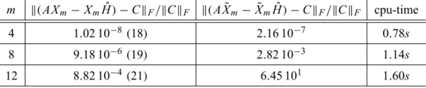
In Table 4.3, we reported the Frobenius norms of the residuals corresponding to the approximations Xm and X˜m for different values of the parameterm, the
total number of iterations (in parentheses) and the required cpu-time.
m k(A Xm−XmHˆ)−CkF/kCkF k(AX˜m− ˜XmH)ˆ −CkF/kCkF cpu-time
4 1.02 10−8(18) 2.16 10−7 0.78s
8 9.18 10−6(19) 2.82 10−3 1.14s
12 8.82 10−4(21) 6.45 101 1.60s
Table 4.3 – Results obtained for the second choice in Example 2.
As can be seen from Table 4.3, the results obtained withXmare more accurate
than those given by the approximation X˜m.
Example 3. The last example describes a model of heat flow with convec-tion in the given domain. The matrix A, is obtained from the centered finite difference discretization of the operator
L(u)=1u− y ∂u ∂x −2x
∂u ∂y −x y
2 u,
on the unit square[0,1] × [0,1]with homogeneous Dirichlet boundary condi-tions. The dimension of the matrixAisn=n2
0wheren0=70 is the number of inner grid points in each direction. As the eigenvalues ofAare large, we divided the matrix AbykAk1. For this experiment, we usedμi = −i; i =1, . . . ,m
(r,m) k(A Xm−XmH)ˆ −CkF/kCkF λ(Hm− f emT)−μk/kμk cpu-time
(2,8) 8.39 10−15(271) 1.01 10−11 17.8s (4,10) 2.90 10−14(273) 5.96 10−10 28.3s (7,13) 2.52 10−14(272) 5.27 10−8 43.5s,
Table 4.4 – Results for Example 3.
5 Conclusion
A global Arnoldi method, suitable for large and sparse computing, is proposed for the solution of the multi-output Sylvester-Observer equation arising in state-estimation in a linear time-invariant control system. The method can be con-sidered to be a generalization of the Arnoldi-method proposed earlier by Datta and Saad in the single-output case. The proposed method is developed by ex-ploiting an interesting relationship between the initially chosen block-row vector and the block-row vector obtained aftermsteps of the global Arnoldi method. This relationship holds for the standard Arnoldi method but does not seem to hold, in general, for the standard block Arnoldi method. The method has the additional feature that the solution produced is F-orthonormal and in the single-output case the obtained solution is the same as the one obtained by the standard Arnoldi method. A numerical stability analysis of the method, as is done in the single-output case by Calvetti, Reichel and the co-authors earlier, is in order.
REFERENCES
[1] C. Bischof, B.N. Datta and A. Purkyastha, A parallel algorithm for the Sylvester-Observer matrix equation. SIAM Journal on Scientific Computing,17(1996), 686–698.
[2] A. Bouhamidi and K. Jbilou, Sylvester Tikhonov-regularization methods in image restora-tion. JCAM,206(1) (2007), 86–98.
[3] R. Bouyouli, K. Jbilou, R. Sadaka and H. Sadok, Convergence properties of some block Krylov subspace methods for multiple linear systems. J. Comp. Appl. Math.,196(2006), 498–511.
[4] D. Calvetti and L. Reichel, Application of ADI iterative methods to the restoration of noisy images. SIAM J. Matrix Anal. Appl.,17(1996), 165–186.
[6] J. Carvalho and B.N. Datta, A block algorithm for the Sylvester-Observer equation arising in state estimation. Proc. IEEE Conf. Dec. Control, Orlando, Florida (2001).
[7] B.N. Datta and K. Datta,Theoretical and computational aspects of some linear algebra prob-lems in control theory, in: C.I. Byrnes, A. Lindquist (Eds.), Computational and Combinatorial Methods in Systems Theory, Elsevier, Amsterdam, pp. 201–212 (1986).
[8] B. N. Datta, An algorithm to assign eigenvalues in a Hessenberg matrix: single-input case. IEEE, Trans. Autom. Contr.,AC-32(1987), 414–417.
[9] B.N. Datta and Y. Saad, Arnoldi methods for large Sylvester-like observer matrix equa-tions, and an associated algorithm for partial spectrum assignment. Linear Algebra and its Applications,154-156(1991), 225–244.
[10] B.N. Datta and C. Hetti,Generalized Arnoldi methods for the Sylvester-Observer equation and the multi-input pole placement problem, in Proceedings of the 36thIEEE Conference on Decision and Control, IEEE, Piscataway, pp. 4379–4383 (1997).
[11] B. N. Datta and D. Sarkissian,Block algorithms for state estimationand functional observers, in Proceedings IEEE Conf. Control Appl. Comput. aided Control Syst., pp. 19–23 (2000). [12] B.N. Datta,Numerical Methods for Linear Control Systems Design and Analysis, Academic
Press (2003).
[13] M. Epton, Methods for the solution of A X D− B X C = E and its applications in the numerical solution of implicit ordinary differential equations. BIT,20(1980), 341–345. [14] C.W. Gear,A simple set of test matrices for eigenvalue programs. Math. Comp.,23(1969),
119–125.
[15] G.H. Golub, S. Nash and C. Van Loan, A Hessenberg-Schur method for the problem A X+X B=C. IEEE Trans. Autom. Control, AC,24(1979), 909–913.
[16] M. Heyouni, The global Hessenberg and global CMRH methods for linear systems with multiple right-hand sides. Numer. Alg.,26(2001), 317–332.
[17] M. Heyouni and K. Jbilou,Matrix Krylov subspace methods for large scale model reduction problems. Applied Mathematics and Computation,181(2) (2006), 1215–1228.
[18] N.J. Higham,The Matrix Computation Toolbox. http://www.ma.man.ac.uk/∼higham/mctoolbox.
[19] R.A. Horn and C.R. Johnson,Topics in Matrix Analysis. Cambridge Univ. Press, Cambridge (1991).
[20] C. Hyland and D. Bernstein, The optimal projection equations for fixed-order dynamic compensation. IEEE Trans. Contr.,AC-29(1984), 1034–1037.
[21] K. Jbilou, A. Messaoudi and H. Sadok, Global FOM and GMRES algorithms for matrix equations. Appl. Num. Math.,31(1999), 49–63.
[23] K. Jbilou, An Arnoldi based algorithm for large algebraic Riccati equations. Applied Mathematics Letters,19(5) (2006), 437–444.
[24] T. Kailath,Linear Systems. Prentice-Hall, Englewood Cliffs (1980).
[25] D.G. Luenberger, Observers for multivariable systems. IEEE Transactions on Automatic Control,AC-11(1966), 190–197.
[26] Y. Saad and M.H. Schultz, GMRES: A generalized minimal residual algorithm for solving nonsymmetric linear systems. SIAM J. Sci. Statis. Comput.,7(1986), 856–869.
[27] P. Van Dooren, The generalized eigenstructure problem in linear system theory. IEEE Transactions on Automatic Control,AC-26(1981), 111–129.
[28] P. Van Dooren,Reduced order observers: A new algorithm and proof. System Control Lett.,