Estud. Econ. vol.33 número2

Factor Productivity

Arilton Teixeira

Associate Professor. Ibmec, Department of Economics

RESUMO

Este artigo analisa se políticas comerciais podem explicar diferenças na produtividade total dos fatores (PTF). É construído um modelo dinâmico com dois setores e com comércio internacional onde a adoção de novas tecnologias é decidida por uma coalizão de trabalha-dores. Os resultados mais importantes são os seguintes:

( )

i com livre comércio ou tarifa

a melhor tecnologia é sempre usada e a PTF está sempre no máximo nível. Com quota, isto não ocorre e a PTF está geralmente abaixo de seu ponto máximo;

( )

ii ainda controlando

para diferenças de habilidade do trabalho (nível de capital humano), trabalhadores na economia com quota têm produtividade menor do que na economia com livre comércio ou tarifa.

PALAVRAS-CHAVE

coalizão, comércio, tecnologia, adoção

ABSTRACT This paper examines if trade policy can account for the difference in total factor productivity (TFP) across countries. A two-sector dynamic international-trade model is developed where technological progress is neutral and a coalition of workers can stop the adoption of new technologies. The key findings are the following: ( )i With free trade, or

tariff, the best technology is always used and TFP is always at its highest value. Under a quota, this is not always the case and TFP is generally below its highest value;

( )

ii even

controlling for difference of skilled labor (or human capital), workers from the quota economy have smaller productivity than workers from the free trade economy.

KEY WORDS Coalition, trade, technology, adoption

INTRODUCTION

It has been well documented that the technological level (TFP - total factor productivity) differs over time and across countries at the industry level or at the national level.1 _{In this paper we develop a dynamic international} trade model to try to account for this persistent difference in TFP. We assu-me that the knowledge that is being used by the workers of the most productive countries are available to be used by the workers of any country, in particular by the workers of the less productive countries.2

We combine two factors to explain the TFP difference across countries: institutional arrangements and trade policies.3 _{On the one hand, the} institutional arrangement allows a group to stop the use of new technologies. On the other hand, the trade policy determine if it is optimum for this group to stop or not the adoption of new technologies.

We construct a two sector growth model with international trade. In both sectors there is exogenous technological progress. In every period a new and more productive technology is available. Also in both sectors the firms behave competitively. But the technology used in these sectors differs. One sector uses skilled and unskilled labor. The productivity of skilled workers is higher, since we assume that only them have the skills to use the newest technology available. In this sector unskilled workers just can use technologies that have been used and abandoned before. Therefore, we assume that only the skilled workers have the power, as group, to decide if the new technology will be used or not. The other sector uses unskilled labor. We assume that every worker can supply unskilled labor and, as a consequence, that workers of this sector cannot block the adoption of new technologies.

1 See PRESCOTT (1998), HARRIGAN (1996;1997) and DOLLAR & WOLF (1993). 2 BAILY & GERSBACH (1995) and BAILY (1993) did not find evidences to justify differences

in productivity by differential access to proprietary technology.

Given this environment we study the effects of three different trade policy: free trade, tariff and quota. The results are the following: ( )i the TFP of

the sector intensive in skilled labor is higher under free trade and tariff than under quota;

( )

ii even controlling for difference of skilled labor (or human capital), workers from the quota economy have smaller productivity than workers from the free trade economy. The intuition for this results is the following. Under free trade and tariff the domestic prices are determined in the international market. Besides, domestic firms are in direct competition with productivity leaders. Skilled workers do not stop the adoption of technology, since given the price for the good that they produce, if they use the most productive technology they maximize their income (and their utility). On the other hand, under quota, prices are determined internally. Stopping the adoption of new technologies increases the relative price of the good that skilled workers produce, increasing their income (and their utility). Since under the quota arrangement the best technology generally is not used, the TFP of the quota economy is smaller. Besides, since the best technology generally is not used the skilled workers are not as productive as the skilled workers of the free trade economy.

occur. In the second there will be no resistance. In this respect, our model show that these different policies have very different outcomes. Last but not least, our generalizations allow us to compute TFP time series under these different trade arrangements and compare them with the data.

This paper is divided into five sections (including this introduction). In Section 1, we develop a model that studies the adoption of technology. First we study an economy under free trade, that is, there are no barriers to trade with other countries. Then, we study the same economy with tariffs. Finally, we study this economy with quota. Section 2 we make a comparison between the equilibrium results of the free trade economy, the tariff economy and the quota economy. Section 3 offers some quantitative results from computer simulations of the models developed in section 1. Last Section concludes.

1. THE ECONOMY

There are two types of agents, i = 1,2 and the measures of the type i are

o

i >

λ

. A type

( )

i agent is endowed with one unit of time of labor of type

( )

i . We assume that the labor of type 1 is unskilled and the labor of type 2 is skilled. At each date, there are two goods y and z.

There is no borrowing and lending and no capital accumulation. The only dynamics of the model is the equilibrium selection of policies (that is, the selection of technologies that will be used). As we will see, to solve the dynamic policy selection problem, it is necessary to determine the competitive outcome within the period given the selected technology.

The period commodity space is

L

=

R

5 with a point in L being

(

y

,

z

,

l

y

,

l

z1

,

l

z2

)

x

=

. y and z are the total amount of each of these goods, y

l is the amount of labor used to produce good y and

l

zi the total amount

uses the labor. The reason why we have these differences will become clear when we specify the technology sets and the policy arrangement.

The consumption set of a type 1 is

{

}

1 : y z1 1, z2 0

X = ∈x L₊ l + ≤l l =

(1)

The consumption set of type 2 is

{

}

2 : y z1 z2 1, z1 0

X = ∈x L₊ l + +l l ≤ l =

(2)

y

l is the amount of labor supplied by a worker to industry y and

l

zi is the amount of labor supplied to industry z by a worker of type i= 1,2. We

should notice that there is no difference between type 1 and type 2 in the y industry. The reason is that we are assuming that this industry just uses unskilled labor and any worker can supply it. Clearly, in equilibrium is not optimum for a type 2 to supply unskilled labor for the z industry.

Preferences

The period utility function for both types is

( )

,

(

y z

1

)

u y z

ρ α α

ρ

−

=

(3)

where y,z≥0 and

ρ

≤1. Besides, we are assuming that preferences are time separable. In a dynamic environment preferences are represented by

(

)

1

0

t t t t

y z

α α ρ

β

ρ

− ∞

=

Technologies

There are three technologies. The first technology produces good y. Its production set is

( )

{

}

3 : , 0

t y

X t = ∈x L₊ y≤

π

l z=

(5)

where

π

>1. An implication of Equation

( )

5

is that there is an exogenous technological progress in the yproduction sector.

The second technology produces good z.Its production set is

( )

{

}

4 , : 1 2, 0

a b

z z

X a b = ∈x L₊ z≤

γ

l +

γ

l y=

(6)

where

γ

>1. Elements a<b are integers that index the z-production in a period. These elements are determined by past policy selections. We are assuming that

γ

>

π

. We should notice that in the z industry workers are different. A Type 2 worker, the skilled type, is more productive and a type 1, the unskilled type.

The third is a foreign trade technology that transforms one good into the other at a rate *

zt

p in period t. Its technology set is

( )

{

*

}

5 : zt 0, ,y z1, z2 0

X t = ∈x L y+ p z= l l l ≥

(7)

The implications of this technology assumption are that there are no borrowing or lending and no transportation cost.

The rate at which z can be transformed into y with international trade is

*

t zt

p

n

π

γ

 

=  

We are treating the rest of the world as a competitive environment. That is, all agents are price takers. Therefore, the relative price of good z(in units of good y) is equal to the ratio of the marginal cost of z and y. Since we have technological progress the path of this ratio is given by the ratio of the technological progress

(

π

over

γ

)

in both sectors. The constant n

represents the constant part of the ratio of the marginal costs in sectors z

and y.

The reason why ownership of technologies is not considered is that all technologies displays constant return to scale. Therefore, profits in equilibrium must be zero.

Policy Arrangement

The integers a and b, where a<b index the technology set

X

₄

( )

a

,

b

, which produces good z. These integers a and b at date t belong to the set

{

0

,...,

t

−

1

,

t

}

.

During the period t, type 2 decides what technology to use next period; that is, type 2 chooses

b

′

∈

{

b

,...,

t

,

t

+

1

}

. If b′>b, that is a better technology is selected, then

a

′

=

b

. If, however, b′=b, then

a

′

=

a

. Thus, if the type 2 choose a better technology the type 1 gain access to the technology that the type 2 were using. If the type 2 choose to continue using the b technology, type 1 does not get access to the b technology.4

Definition

We will say that the group of type 2 is blocking the adoption of new technologies or there is blocking of technologies if

b

<

t

.

1.1 Period Competitive Equilibrium

To facilitate the understanding of the definition of equilibrium, we can divide it in two parts. One part is static and competitive. We will call it period competitive equilibrium. In this part, agents take the prices as given to maximize their objective functions. The other part is dynamic. The period competitive equilibrium can be determined as a function of the state variables

s

=

(

a

,

b

,

t

)

, since there is no borrowing or lending and no capital accumulation.5

A period competitive equilibrium is a price system p =

(

py,pz,wy,wz1,wz2

)

, allocations

{ }

x

ˆ

i 5_i=1, imports and exports

{

y

ˆ

*

( ) ( )

s

,

z

ˆ

*

s

}

such that, given

( )

*

, 1pz , the external prices of the goods y and z

(i) For

i

x

i

=

1

,

2

,

ˆ

maximizes

u

(

y

,

z

)

s.t.

i _i

X

x ∈

y+ pzz ≤wylyi +wzilzi

(ii) For

j =3,4,5

{

j

}

j z z z z y y z y j

X

x

l

w

l

w

l

w

z

p

y

p

x

ˆ

∈

arg

max

+

−

−

_{1 1}

−

_{2 2}

:

∈

(iii) Market Clearing

2 3 4 5

2 1

1xˆ +

λ

xˆ = xˆ +xˆ +xˆ

λ

1.2 Dynamic Equilibrium

Now, let us study the dynamic part of our equilibrium. Type 2 collectively chooses whether to shift to a better technology or not.6

5 In the subsequent definition of equilibrium the

s

argument is implicit for all the equilibrium elements.

The dynamic programming of this group can be written as

( )

max

{

( )

( )

}

b

v s

U s

β

v s

′

′

=

+

s.t.

b

≤

b

′

≤

t

+

1







=

′

>

′

=

′

b

b

if

a

b

b

if

b

a

,

,

(9)

(

′

,

′

,

+

1

)

=

′

a

b

t

s

where U

( )

s ∈R is the period equilibrium utility of a type 2.7

Dynamic Recursive Equilibrium

A dynamic recursive equilibrium is a set of price functions

( ) ( ) ( ) ( ) ( )

{

p s p s w s w s w s

}

p = _y , _z , _y , _z1 , _z2 , a value function v

( )

s , allocations

functions for consumers

{

y

₁

( ) ( ) ( ) ( )

s

,

y

₂

s

,

z

₁

s

,

z

₂

s

}

,

{

l_y1

( ) ( ) ( ) ( )

s,l_z1 s,l_y2 s,l_z2 s

}

,

allocations functions for firms

{

ly

( ) ( ) ( )

s ,l1 s,l2 s

}

, a transition dynamics

function g(s) and imports and exports

{

y

*

( ) ( )

s

,

z

*

s

}

, such that: consumers maximize utility, firms maximize profits, markets clear. In addition, function

( )

s

v satisfies (9).

1.3 The Economy With Free Trade

In this section we will study the equilibrium path for this economy. We are assuming the Home Country, is a small open economy8 _{and there is no}

7 For the case of the parametric class of economies considered here the period equilibrium exists, is unique and

U

( )

s

is a function.

transportation cost or any other cost to trade with the rest of the world. The state variable s determines the available technologies. Consequently the endogenous variables are function of

s

. In the following exposition this function dependency is implicit, unless it can create some misunderstanding.

To study the equilibrium path of this economy we have to find the optimum decision rule for the type 2 group, that is, we need to specify

s

′

=

g

( )

s

. Given

g

( )

s

the other choice variables can be determined. The specification of

g

( )

s

is introduced in Proposition 1. The rest of the proof of the existence of Dynamic Recursive Equilibrium is presented in Proposition 2.

Before we go any further we should explain one point. Since both types of workers can work in both sectors, in equilibrium we could have different distribution of workers across sectors. In what follows, we will look for an equilibrium path where there is a complete specialization of workers. That is, workers of type 1 work in the production of good y and workers of type 2 work in the production of good z. This approach facilitates our proofs but our results do not depend on this specialization. We will prove the existence and uniqueness of an equilibrium for this case, since we will focus our analysis in this segregated equilibrium (the same proof can be extended to the other cases).9

The next proposition shows that under free trade, workers of type 2 will not block the adoption of new technologies. The intuition for this result is the following. First, the higher is the income of a type 2 agent, the higher is his consumption and his utility. The income of a type 2 is equal to the marginal productivity of labor of type 2 times the price. With free trade, the internal price is exogenous since it is given by the price in the rest of the world. Therefore, the higher is the marginal productivity of labor of type 2 the higher is his income. Given the production function, the group of type 2 has to pick the highest possible value for b, that is

b

=

t

.

Proposition 1: If there is free trade, that is the agents have access to the

X

₅

( )

t

technology and 1≤n≤

γ

, then the best strategy for workers of type 2 is not

blocking the adoption of the new technology. That is,

b

=

t

, for all t.

Next proposition will conclude the proof of the existence of a dynamic recursive equilibrium under free trade. The intuition is straightforward once we understand Proposition 1. That is, since there is no blocking there is technological progress and growth. We define

β

~

≡

β

(

γ

1−α

π

α

)

ρ_.

Proposition 2: If 1≤n≤

γ

,

β

~∈

( )

0,1 and there is free trade, then there is a

unique dynamic recursive equilibrium where all of type 2 work in the z industry

(that is,

l

_z1

=

0

,

l

_z2

=

λ

₂) and

* *

1 1 1

t it t

t it t

y

y

y

y

₋

=

y

₋

=

y

₋

=

π

(10)

* *

1 1 1

t it t

t it t

z

z

z

z

₋

=

z

₋

=

z

₋

=

λ

(11)

By a balance growth path we mean an equilibrium where all variables are growing at a constant growth rate. From Proposition 2, more specifically, from Equations

( ) ( )

10 − 11 we see that in equilibrium the free trade economy is in a balance growth path.

2.4 The Economy With a Tariff

In this subsection we will introduce a tariff on the imports of good z. Then we will analyze what happens in this economy with respect to adoption of technology.

z were not imported when the tariff was zero, nothing would change if a tariff is imposed on the imports of z. Let

α

α

α

λ

λ

λ

λ

λ

n

and

+

−

−

≡

′

+

≡

1

1

2 1

2

Proposition 3: If 1≤n≤

γ

, there is no borrowing or lending and there is no

barriers to trade among countries then:

( )

i

If

λ

>

λ

′

, the Home Country will export good z;

( )

ii If

λ

<

λ

′, it will import good z;

( )

iii If

λ

=

λ

′, there is no trade.

The intuition of the proposition above is as follows. Given the relative prices and the preferences, the larger is

λ

, the larger is the production of good z. Therefore, if

λ

is very high the Home Country would export good z. On the other hand, given

λ

, if

α

is small, that is, if

λ

is big, then the proportion of the income spend on consumption of good z is big and the Home Country will be an importer of good z.

It should be noted that the results given by Proposition 3 is in agreement with the Heckscher-Ohlin Theorem. That is, if

λ

is high, the country tends to be an exporter of good z.

Now, suppose that the government imposes a tariff τ on imports of good

z. In this case, without any transportation cost or any cost to trade between countries, we have

(

)

*

1

zt zt

p

= +

τ

p

(12)

where * zt

With the introduction of a tariff the definition of a equilibrium will change. But, I will not repeat the definition here, since we just need to introduce a sequence

{ }

τ

t ∞_t=o of tariffs and the fact that pzt is given by Equation (12). Moreover, I am assuming that the government throws away the income that it collects from the tax over the imports. Therefore, the market clearing conditions will not change.

Given the linearity of the production functions used here, the introduction of a tariff can have big effects in the internal production of goods y and

z. The following proposition show these changes.

Proposition 4: If

( )

i 1≤n≤

γ

;

( )

ii

λ

<

λ

′;

( )

iii transportation costs are

zero; and

( )

iv

the government introduces a tariff in the imports of good z

then in equilibrium

( )

i

If

γ

<

(

1

+

τ

)

n

then, there is no production of good y. In this case, the growth rate of the production of good z in period T is

1

1 2

t t

z z

λ

γ

λ

−

= +

₍₁₃₎

and for

t

>

T

,

z

t

/

z

t₋1

=

γ

( )

i

If

γ

< +

(

1

τ

)

n

, there is no reallocation of workers between sec-tors. The growth path of the variables of this economy is still given by Equations (10) — (11).

In any case given by Proposition, after the introduction of a tariff we still have some effects over the relative wages. This is shown in the corollary below.10

Corollary 1: Take all the assumptions of Proposition 4. If there is an introduction of a tariff in the imports of good y, then there is an increase in the relative wage of the workers of type 2 with respect to the workers of type 1.

With the wedge that the tariff creates between the internal and the external prices, there is room for the group of the workers of type 2 to block the adoption of new technologies. But, as we will see below, the introduction of a tariff is not sufficient to make the workers of type 2 to block the adoption of the new technology in the sector that produces good

z

. The intuition is the same given for Proposition 1. That is, since the internal price is defined by Equation (12), any resistance to new technologies will just reduce the marginal productivity of labor of type 2, reducing the income of workers of type 2.

The above ideas are the intuition behind the next proposition. Remember that we define β~_≡β

(

γ1−απα

)

ρ_.

Proposition 5: If

( )

i 1≤n≤

γ

;

( ) (

ii

β

~∈ 0,1

) ( )

; iii

λ

<

λ

′;

( )

iv trans-portation costs are zero; and

( )

v

the government introduces a tariff in the imports of good z, then there is a dynamic recursive equilibrium where workers of type 2 do not block the adoption of new technologies.

Proposition 5 shows that as long as the internal price of good z is linked with the external price as in Equation (12), then it is never an optimal choice for workers of type 2 to block the new technology. In this case, the block of new technologies will just have the effect of reducing the marginal productivity and the income of a type 2 worker. The important conclusion here is that in our model, for any level of tariff, the connection between internal and external prices is not broken.11

One way to break the linkage between the external and the internal price is through the introduction of non-tariff barriers such as quotas. Therefore, in the next section we will try to see how the introduction of a quota in the international trade can interfere in the technology adoption.

2.5 The Economy With a Quota

Suppose now that the government in the Home Country introduces a quo-ta

Q

zt in the imports of good z.12 I will assume that only the government has the right to import and export. The income that the government collects, given by the difference between internal and external prices, is thrown away.13

The introduction of a quota changes our previous framework. First, since we do not have borrowing or lending, from the equilibrium condition of the Balance of Payment we get

zt yt zt

t

Q

p

p

y

_















−

=

_**

*

Second, we should define

Q

zt. To be effective, that is, to reduce the imports

of good z,

Q

zt has to be smaller than the amount that would be imported if we had a free trade. From Equations (10) — (11), in a balance growth path, zt /zt

*

is constant. Defining * *

/ t ≡Λ t z

z , we will define a quota as a proportion of the domestic production, that is

12 Clearly, this discussion makes sense only if the Home Country is an importer of good z. Therefore, in this section we are assuming that the Home Country is an importer of good z. Following the notation developed in the section before, we are assuming that λ<λ′.

zt zt

Q

= Λ

(15)

where

(

*

)

,

0 Λ

∈

Λ .

Finally, since a quota breaks the link between the internal an the external price, we need to determine the internal price of good z (price of good y

is taken as numeraire). The production of z will increase in the Home Country with the introduction of a quota. This increment is made through switching labor of type 1 from the y sector to the

z

sector. But, in equilibrium it can not exist any wage differential between type 1 in the y

and in the

z

sector. That is, in equilibrium we would have

1

y z

w =w

(16)

From Equation

( )

16 and the firm’s problem

t zt a

p

π

γ

=

(17)

Given the above changes, now I will show that with the introduction of a quota, the workers of type 2 will be better off if they block the adoption of the new technologies. In the next proposition,

d

≡

b

−

a

is the difference of age between the technology used by workers of type 2 and the technology used by workers of type 1 working in the production of good z. In equilibrium this difference will be constant.

Once a quota is introduced the linkage between internal and external prices are broken. But, we still have a maximum number of periods that workers of type 2 could block the new technology. First, because the opportunity cost of not using the newest technologies available increases as the sector

z falls behind the frontier. Second, because we are assuming that the coalition of type 2 has to treat each type 2 equally and therefore it will keep every type 2 working in the z sector.14 _{Therefore, if z is very far from the}

frontier pzt is too high and the quantity demanded of good z is smaller

than the amount produced by the type 2 workers. The upper limit generated by the last assumption is given by the equilibrium in the domestic market of good z. Using the market clearing condition for good z and Equation (15) we get an upper bound for

d

.

(

)

(

)

1 2

log

1

log

log

d

λ

α

λ α

d

γ

−

−

+ Λ

















≤

≡

(18)

It is straightforward from Equation (18) how

α

and

Λ

affect d. But, Equation (18) also shows two other important relations. First is the relation between the size of the group that can block

( )

λ

₂ and the size of the rest of the country

( )

λ

₁ in the decision whether to resist or not to new technologies. As we will see in Proposition 6, a group finds better to resist new technologies the bigger is d. In Equation (18), given

λ

₂, the bigger is

λ

₁ the bigger is d. In this case, it is better for type 2 to resist new technologies. The intuitive reason for this result is as follows. It is good for type 2 to block the adoption of new technologies because the blocking increases the price of good

z

, transferring income from the rest of society

( )

λ

1 to type 2 group

( )

λ

2 . If the rest of society

( )

λ

1 is small this transfer is very small. In this case it is not optimum blocking since the increment of

ρ

zt harms any type 2 as a consumer.

The second relation showed by Equation (18) is between the rate at which the technology is advancing

( )

λ

and the decision to resist new technologies. As we can see in Equation (18), if the technology is advancing very fast it is not optimal for the type 2 group to resist (since d is very small). The intuition is that the bigger is

( )

λ

, the bigger is the opportunity cost to resist to new technologies.

Proposition 6:

If

0,1 ,

β

%

∈

( )

λ λ′

<

, and that the government introduces a

quota in the imports of good

z

then for d,

α

and

β

~

sufficient large the workers

of type 2 will block the adoption of the new technology for any value of

ρ

.

We could state the maximization problem of type 2 group using a Bellman equation. In this case we would have (define

=

1

−

d

)

( )

(

( )( )

)

( )

















′

+

=

− − + +

′

s

s

v

_v

d a t d

b 2

~

max

1

2

β

ρ

γ

α α ρ

(19)

s

.

t

.

d

₋

≤

d

≤

d

Clearly, type 2 group would block if

α

,

β

~

and

d

are large enough.

We should stress some points. First, once a quota is introduced the country will have less trade. That is, the ratio of export plus imports over GDP reduces. Second, Equation (18) shows that big groups of small countries, independent of the institutional arrangements of these countries, have less incentive to block the adoption of new technologies. On the other hand, small groups of large countries will demand much more protection from the external competitors.

2. COMPARISONS OF FREE TRADE, TARIFF AND QUOTA

Generally there is an equivalence between tariff and quota. That is, for a given tariff, there is a quota that generates the same amount imported and the same internal price. Besides, equivalent to a quota equal to zero, there is a minimum level of a tariff above which there is no international trade and the internal price is set independent of the external price.15

Let us check if there is a tariff that generates the same price level of the quota economy (and therefore the same consumption of both goods). That is, is there a

τ

such that

(

)

t

a t

n









+

=

γ

π

τ

γ

π

1

_{? To answer this question, just rearrange the above}

expression to get

1

−

=

−

n

a t

γ

τ

In the above expression

τ

is a function of time, since

t

−

a

is not constant. Under the economy with quota

a

is constant for many periods and

t

is varying. Therefore, for the case studied here where

τ

is constant, there is no equivalence between the economy with quota and the economy with tariff.

Finally, a quota equal to zero shuts down the international trade in the Quota economy. As we saw, there is no tariff (finite number) that can shut down international trade in the economy with tariff. As tariff increases the economy moves from importer of good

z

to exporter of good

z

and trade still happens.

In our model, there is no equivalence between tariffs and quotas with respect to the adoption of new technologies. As we saw in Proposition 4 with tariff there is a linkage between internal and external prices. For

τ

=0 the Home Country imports good

z

. Once we start raising

τ

the domestic price of

z

also starts increasing

(

p

z

=

(

1

+

τ

)

p

z*

)

, reducing domestic consumption of

z

. We can keep raising

τ

, reducing consumption of

z

, until domestic production and domestic consumption of good

z

are equal (that is, there is no trade). After this point new increments in

τ

will have no effect on the domestic price of

z

. To see this notice that if the domestic price of

z

would increase above the value for which domestic supply equal domestic consumption the Home Country would become an exporter of

than the international price. Therefore all producers would try to sell in the domestic market, reducing the domestic price until supply is equal demand. In any case, since for any value of

τ

the coalition of workers cannot affect domestic prices, the best strategy for any level of tariffs is to use the best technology available.

On the other hand, after the introduction of a quota the internal and the external prices of good

z

differ since the quota breaks the connection between them. The reason for this change in prices is the following. To move workers of type 1 from the

y

_{sector to}

z

_{sector the wage paid to a}

type 1 must be equal among these sectors. Since a quota has to reallocate the workers the internal price of

z

is set in a way to guarantee this equalization. In this case, workers of type 1 are indifferent between where to work. Since they are indifferent, in equilibrium they are allocated across sectors to satisfy the demand for both goods.

3 COMPUTER SIMULATION

In this section we will analyze the results from the computer simulation of the model under the free trade policy and under the quota policy.16

Before we start the analysis, we want to explain some points. First, we are not doing a calibration exercise. Instead, we just want to show the potential of the model to explain persistent quantitative differences in TFP. The values of the parameters were chosen to satisfy the assumptions of the propositions proved before. To have a more rigorous analysis we would need data that unfortunately are not available.17 _{Second, we just carry sensitive analysis}

16 Since the conclusions of the tariff arrangement is the same as the free trade arrangement I will not repeat then here.

for changes in

Λ

because the results are not very sensitive for changes in the other parameters.

Third, the TFP for the

z

sector of our model economy is computed in the following way. It is a weight average of

γ

a _and

γ

b_{. That is,}

(

)

b a

TFP

=

ξγ

+

1

−

ξ

γ

(01)

where

2 1

1

z z

z

l

l

l

+

=

ξ

. The TFP, as computed above, is the product per worker

in the z sector. We can see this looking at the production set of good

z

.

Third, after each variable we introduce a letter

f

or

q

_{indicating that the}

value of the variable is from the free trade economy or the quota economy, respectively. For example, TFP

f

( )

t

is the value of the TFP of the

z

sector in the free trade economy in period

t

.

Using the above notation and the parameter values shown in Table 1, we get the following results:

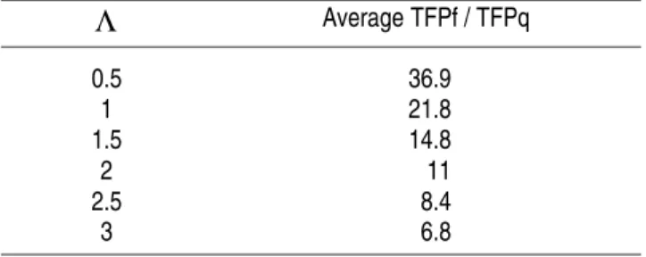
1) The TFP of the

z

sector is smaller in the quota economy than in the free trade economy. This difference increases with the level of protec-tion. The smaller is

Λ

(more protection) the bigger is the difference in TFP between the quota and the free trade economy (see Table 2).

2) Even controlling for difference in the skill levels, workers in the quota economy are less productive than workers in the free trade economy (see Table 3).

The intuition behind these results is the following. With free trade, the price is determined in the international market. Domestic producers are in competition with foreigner producers that are using the best technology available. In this case skilled labors do not stop the adoption of new technologies, since given the prices, producing with the most productive technology available maximizes their income and their utility.

With quota, the domestic price is set independent of the international price. Skilled workers can increase the relative price of the good that they produce, stopping the use of new technologies. In this way, they increase their income and their utility.

CONCLUSIONS

In this paper we try to explain why the TFP differs over time and across countries. To answer this question we used institutional arrangements and international trade.

The institutional arrangement would allow groups to stop the adoption of new technologies. The trade policy would make it optimum or not to exercise this power. International trade (free trade) would generate competition among firms independently of the country where they are producing.

In our model economy, the TFP of free trade economies would be higher than TFP of closed economies. The reason is that firms operating under free trade policy would always use the most productive technology available. Under free trade the workers would not stop the adoption of new technologies. The same is also true for economies with tariff.

On the other hand, under the quota arrangement the skilled workers can increase the relative price of the good that they produce if they stop the adoption of new technologies. In this case, firms will be using old and less productive technologies. Therefore, under the quota arrangement the TFP of the protected sector is always smaller than the TFP of this sector under the free trade (and tariff) arrangement.

Finally, even controlling for difference in the skill level of workers the productivity is smaller under the quota agreement than under the free trade agreement. That is, the skilled workers are less productive under the quota agreement than under the free trade agreement. The reason is the use of old technology by the skilled workers when new and more productive technologies were already available. This result is in line with the well documented difference in productivity across countries, even when we control for differences in human capital.

Finally for future research we should add capital in the model. Clearly, this would add another constraint for the coalition of workers. With capital, resistance to new technologies would reduce marginal productivity of ca-pital, reducing investment and the capital labor ratio. Therefore, we should expect that with capital, the resistance should reduce (the distance from the frontier d, should be smaller for the same levels of trade barriers).

REFERENCES

BAILY, M. Competition, regulation and efficiency in service industries.

Brookings Papers on Economic Activity, Microeconomics, p. 71-103,1993. BAILY, M.; GERSBACH, H. Efficiency in manufacturing and the need for global competition. Brookings Papers on Economic Activity, Microeconomics, p. 307-347, 1995.

CUNHA, Alexandre; TEIXEIRA, Arilton. The impacts of trade blocks and tax reforms on the Brazilian economy. In: Anais do Encontro Brasileiro de Econometria, volume 1. Sociedade Brasileira de Econometria, 2002.

DEBREU, G.; SCARTF, H. A limit theorem on the core of an economy.

DOLLAR, David; WOLFF, Edward N. Competitiveness, convergence, and

international specialization. MIT Press, 1993.

HARRIGAN, James. Cross-country comparisons of industry total factor productivity: theory and evidence. Federal Reserve Bank of New York, 1996. Mimeo.

_______. Estimation of cross-country differences in industry production functions. Working Paper 6121, NBER, 1997.

HOLMES, T.; SCHMITZ, J. Resistance to new technology and trade between areas. Federal Reserve Bank of Minneapolis Quarterly Review, 19, p. 2-17, 1995.

LUZIO, Eduardo. The microcomputer industry in Brazil. Praeger Publishers, 1996.

PARENTE, S.; PRESCOTT, E. Barriers to technology adoption and development. Journal of Political Economy, 102, p. 298-321, April 1994. _______. Monopoly rights: a barrier to riches. American Economic Review,

89, p. 1216-33, 1999.

PRESCOTT, E. Needed: a theory of total factor productivity. International

Economic Review, 39, p. 525-52, 1998.

WOODLAND, A. D. International trade and resource allocation. North Holland, 1982.

TABLE 1 - PARAMETERS

Parameters Values

α 0.7

ρ 0.5

β 0.96

δ 0.05

γ 1.02

π 1.015

η 1.01

λ1 98

TABLE 2 - TFPF / TFPQ FOR DIFFERENT LEVELS OF PROTECTION

Λ

Average TFPf / TFPq

0.5 36.9 1 21.8 1.5 14.8

2 11 2.5 8.4

3 6.8

TABLE 3 - DIFFERENCE OF PRODUCTIVITY FOR TYPE 2 FOR DIFFERENT LEVELS OF PROTECTION

Λ

Average Difference in Productivity for Type 2

0.5 4.4 1 3.5 1.5 2.9 2 2.6 2.5 2.3 3 2.1

APPENDIX

Proof of Proposition 1: We are assuming that the Home Country is a small open economy. In this case, the Home Country and the rest of the world will have the same prices (the star indicates the value of a variable in the rest of the world)

*

1

yt yt

p

=

p

=

(20)

* zt zt

p

Since

1

≤

η ≤

γ

it follows that

w

z1

≤

w

y

≤

z2 and

l

z1

=

0

and

l

z2

=

λ

2. Therefore, the income of any labor of type 2 is

p

z

( )

s

λ

b

.

Since

( )

* zt z

s

p

p

=

is exogenously given, the best that workers of type 2 can do is to increase their productivity choosing the most efficient technology, making b =t.

Proof of Proposition 2: With the notation previously defined, the standard techniques to prove existence and uniqueness of equilibrium do not work, since we do not have bounded functions. Therefore, we will redefine the variables making possible to use the bounded return techniques. This proof will follow these steps. First, we will show that the consumers and firms demand functions calculated for the period economy satisfy the market clearing conditions (since they clearly solve the firms and consumers problem of maximization). Then I will show that there exists a unique value function that solves the group 2 dynamic problem, given those functions of the period equilibrium (as before, the functional dependency of

s

is implicit).

Define t t t t t t

z

z

and

y

y

γ

π

=

=

~

~

(22)

t t t t t t

z

z

and

y

y

γ

π

* * * *

~

~

₌

₌

(23)

and for

i

=

1

,

2

t it it t it it

z

z

and

y

y

γ

π

=

=

~

~

(24)

By assumption,

1

≤

η ≤

γ

. But, if

η ≤

γ

, then

w

z1

≤

w

yand the type 1 work in the production of good

y

_{. On the other hand, if}

η

≥

1

then

w

z2

≥

w

y and the type 2 just work in the production of good

z

. This shows that

0

1

=

z

From the technologies defined for production of goods

y

_and

z

and Equations (22) – (24), since

1

≤

η ≤

γ

.

2 1

~

~

₌

_λ

₌

_λ

t t

and

z

y

(25)

Now, let us show that the market clearing condition is satisfied. It is easy to see that the labor markets are in equilibrium. We need to verify for other goods. For good

y

we get

* 1 2 2 1

1

y

y

y

t

+

=

+

λ

λ

π

λ

(26)

Dividing Equation (26) by

π

t, using the definitions given by Equations (24) – (25) and the consumer maximization problem, we get

(

)

b t

y

*

=

−

1

−

α

λ

₁

+

αηλ

₂

γ

−

~

₍₂₇₎

Repeating the some steps for good

z

we get

(

)

b t

z

=

−

α

λ

+

αηλ

γ

−

η

1 2

*

1

~

₍₂₈₎

Adding up Equations (27) – (28), we get from the technological set

X

₅

( )

t

0

0

~

~

*

+

*

=

⇔

*

+

* *

=

z

p

y

z

y

η

_z

(29)

Equations (27) – (29) conclude the proof that markets clear.

From Equations (25), (27) – (29) and the demand functions of the consumers we get the growth rates given by Equations (10) – (11).

(

)

_∑

(

)

∑

∞ = − ∞ = −

=

0 1 2 2 0 1 2

2

~

~

~

t t t t t t t

t

y

z

y

z

ρ

β

ρ

β

ρ α α ρ α α

(30)

where

β

~

∈

( )

0

,

1

by assumption.

From the period equilibrium we get the demand functions for consumer of type 2

y

2t

~

_{and .}

t

z

₂

~

_{Substituting these period demand functions into}

Equation (30) we get

(

_{α α}

)

ρ ρ

γ

β

ρ

β

=

Ψ

∞

_



₋

_



= ∞

=

−

∑

∑

t b

t t

t

t t

t

y

~

z

~

~

1

~

0 0 1 2 2

(31)

where

Ψ

=

[

α

α

(

−

α

)

1−α

]

ρ

1

/

( )

ρ

Define

b

ˆ

=

t

−

b

,

a

ˆ

=

t

−

a

and

t

ˆ

=

0

. The consumers of type 2 problem can be written as

( )

( )

















′

+









Ψ

=

′

v

s

s

v

b b

ˆ

ˆ

1

max

ˆ

_ˆ

ˆ

γ

β

ρ

(32)

Where

b

ˆ

′

∈

X

ˆ

=

{

b

−

t

,...,

t

+

1

−

t

}

=

{

−

b

ˆ

,...,

1

}

. But from Proposition (1),

{ }

0

,

1

ˆ

₌

X

, since b=t.

To prove existence and uniqueness we will work with the convex hull of

X

ˆ

, that we call

X

=

[ ]

0

,

1

. Clearly, X is convex. Now, define

Γ

:X → X

Define, A=

{

( )

bˆ,bˆ′∈X×X_Mbˆ′∈Γ

( )

bˆ

}

and F:A→R₊where F

( )

bˆ,bˆ 1_ˆ F

( )

.,. b ⋅

   Ψ = ′

ρ

γ is continuous and bounded. Therefore, X,

Γ

and F satisfy the assumptions of Theorem 4.6 of Stokey and Lucas (1989). It Follows that there exists a unique value function

v

( )

s

that solves the type 2 problem.

It just remains to be shows that this solution satisfies our original problem, since we use

X

=

[ ]

0

,

1

, instead of

X

ˆ

=

{ }

0

,

1

. But, this comes straightforward, since by Proposition 1, b=t and

Γ

( ) { }

X

=

0

.

Proof of Proposition 3: From the equilibrium condition in the market of good

y

, no trade requires

1 2

2 1

1

λ

π

λ

λ

t

t t

y

y

+

=

The demand for type 1, that is,

y

1t, is t

απ

and the demand

y

2tis t zt

p

γ

α

.

Substitution above yields

(

1

−

λ

)

απ

t

+

λα

p

_zt

γ

t

=

π

t

(

1

−

λ

)

Further transformation with the use of Equation (8)

λ

αη

α

α

λ

≡

′

+

−

−

=

1

1

(33)

Proof of Proposition 4: We will give the following steps in this proof. First, we will show that it is not a optimum strategy for the type 2 to block the adoption of new technologies. Then, given that there is no block, we will show that there exist an equilibrium.

Suppose the government introduces a tariff

τ

in the imports of good

z

in period

T

. To see if the workers of type 2 are better off if they block the new technology we just need to compare the utility from period

T

on.

Call

U

N2 the utility of a representative a gent with labor of type 2 from

period

T

on, when there is no block of the upcoming technology. In the same way, 2

B

U

is the utility of workers of type 2, for the same period, if they block the new technology. Now, since

(

1−

)

<

1

,

y

*t

>

0

ρ α α

_π

γ

β

it follows

that both 2 N

U

and 2 B

U

are finite.

The price of good

z

is given by

(

)

_T T

γ

π

η

τ

+

1

. If the workers of type 2 block

or not the adoption of new technology, the falling in the relative price of good

z

is not affected. On the other hand, the productivity of workers of type 2 will be smaller if they block the new technology. Therefore, the income of workers of type 2 will be smaller in each period if they block the new technology. Since the marginal utility is positive, it is easy to see that workers of type 2 will be better off it they do not block the adoption of the new technology, that is,

U

N2

−

U

B2

<

0

. This concludes the proof that is it

not an optimum strategy to block the adoption of new technologies. Given that there is not block, the proof of the existence of an equilibrium follows the same steps given in the proof of Proposition 2 (therefore, I will not repeat it here). To understand that, notice that we just multiplied the external price by a constant and repeat the same steps.

know that there is an equilibrium for each case where there is no block. Now, suppose that the government introduces a tariff

τ

in the imports of good

z

. If

(

1

+

τ >

)

η

γ

, then

(

)

γ

η

τ

+

<

1

1

and after some manipulations,

(

)

1

1

t

t

π

t

π

τ η

γ

γ

−

 

< +

_{ }

 

Since

w

y

=

π

tand

(

)

1

1

1

−









−

=

t

t

z

w

γ

γ

π

η

τ

it follows that

w

z1

>

w

y. Therefore,

l

_z1

=

λ

₁ and

y

=

0

. Clearly, the reallocation of workers toward the

z

sector from period

T

on explain the growth rate of the

z

sector.

Following the same steps we can show that if

(

1

+

τ ≤

)

η

γ

, then y

z

w

w

₁

≤

_and

_l

_z1

=

₀

_{. That is, in this case the tariff does not effect the}

allocation of workers across sectors.

Proof of Proposition 6: By hypothesis, the Home Country is an importer of good

y

_{and at period}

T

the government introduces a quota. To see if the workers of type 2 are better off if they block the new technology we just need.

This paper is based on my PhD dissertation. I an specially grateful to my adviser Ed Prescott and to Jim Schmitz and berthold Herrendorf. I am also in debt to J. C. Conessa, Carlos Diaz, Ron Edwards and Tim Kehoe. I also thank two anonymous referees for helpful comments and Opencadd for providing a Matlab license. As usual, the remaining mistakes are mine.

Email: [email protected]