Neutrino Mixing as a Source for Cosmological Constant
M. Blasone
♭♯, A. Capolupo
♭, S. Capozziello
♭, S. Carloni
♮, and G. Vitiello
♭♯ ♭Dipartimento di Fisica “E.R. Caianiello” and INFN, Universit `a di Salerno, I-84100 Salerno, Italy♯Unit`a INFM, Salerno, Italy
♮Department of Applied Mathematics, University of Cape Town, South Africa
Received on 19 December, 2004
We report on recent results showing that neutrino mixing may lead to a non-zero contribution to the cosmolog-ical constant. This contribution is of a completely different nature with respect to the usual one by a massive spinor field. We also study the problem of field mixing in Quantum Field Theory in curved space-time, for the case of a scalar field in the Friedmann-Robertson-Walker metric.
1
Introduction
The problem of cosmological constant is currently one of the most challenging open issues in theoretical physics and cos-mology. The main difficulty comes from the fact that, when estimating its value as a gravitational effect of vacuum en-ergy, the numerical results are in strong disagreement with the accepted upper boundΛ<10−56cm−2[1].
We show here that a new contribution to the vacuum en-ergy and therefore to the cosmological constant may arise from neutrino mixing [2]. The contribution we find comes from the specific nature of the field mixing and is therefore of completely different origin with respect to the ordinary vac-uum energy contribution of a massive spinor field.
Indeed, it has been shown [3]-[13] that the vacuum for fields with definite masses is not invariant under the field mix-ing transformations and in the infinite volume limit, it is uni-tarily inequivalent to the vacuum for the fields with definite flavor. In the case of neutrinos, this results in a condensate of neutrino-antineutrino pairs, with a density related to the mixing angle(s) and mass difference(s) among the different generations. Phenomenological consequences of such a non-trivial condensate structure of the flavor vacuum have been studied for neutrino oscillations [8] and for beta decay [9].
In this paper we consider the case of two flavors and Dirac neutrino fields, although the conclusions we reach can be eas-ily extended to the case of three flavors and Majorana neutri-nos [11, 12].
We also include a preliminary study of mixed (bosonic) fields in a curved background, for the case of FRW metric.
In Section 2, we shortly summarize the main results for neutrino mixing in QFT. In Section 3, we compute the neu-trino contribution to the cosmological constant and estimate its value by using the natural scale of neutrino mixing as a cut–off. The result turns out to be compatible with the cur-rently accepted upper bound on Λ. In Section 4, quantum fields and mixing relations are analyzed in expanding uni-verse. Section 5 is devoted to conclusions.
2
Neutrino mixing in Quantum Field
Theory
The main features of the QFT formalism for the neutrino mix-ing are summarized below. For a detailed review see [13]. For sake of simplicity, we consider the two flavor case and we use Dirac neutrino fields. The Lagrangian density describing the Dirac neutrino fields with a mixed mass term is:
L(x) = ¯Ψf(x) (i6∂−M) Ψf(x), (1)
whereΨT
f = (νe, νµ)andM =
µ
me meµ
meµ mµ
¶
. The re-lation between Dirac fieldsΨf(x), eigenstates of flavor, and
Dirac fieldsΨm(x), eigenstates of mass, is given by
Ψf(x) =UΨm(x), (2)
withΨT
m= (ν1, ν2).U is the mixing matrix
U =
µ
cosθ sinθ
−sinθ cosθ
¶
(3)
beingθthe mixing angle. Using Eq.(3), we diagonalize the quadratic form Eq.(1), which then reduces to the Lagrangian for the Dirac fieldsΨm(x), with massesmi,i= 1,2:
L(x) = ¯Ψm(x) (i6∂−Md) Ψm(x), (4)
whereMd =diag(m1, m2). The mixing transformation (2)
can be written as [3]
νσ(x)≡G−θ1(t)νi(x)Gθ(t), (5)
where(σ, i) = (e,1),(µ,2), and the generatorGθ(t)is given
by
Gθ(t) = exp
h
θ
Z
d3x³ν1†(x)ν2(x)−ν†2(x)ν1(x)
´ i
The free fields νi (i=1,2) are given, in the usual way, in
terms of creation and annihilation operators (we uset≡x0):
νi(x) =
X
r
Z d3k
(2π)32
h
urk,i(t)αrk,i +v−rk,i(t)β r† −k,i
i
eik·x,
(7) withi= 1,2,
ur
k,i(t) =e−iωk,iturk,i, vkr,i(t) =eiωk,itvkr,i (8)
andωk,i=
p
k2+m2 i.
The mass eigenstate vacuum is denoted by |0im:
αr
k,i|0im = βkr,i|0im = 0. The anticommutation relations,
the wave function orthonormality and completeness relations are the usual ones (cf. Ref. [3]).
The flavor fields are obtained from Eq. (5): νσ(x) =
X
r
Z d3k
(2π)32
h
urk,i(t)αrk,σ(t)
+ v−rk,i(t)β r† −k,σ(t)
i
eik·x, (9) with(σ, i) = (e,1),(µ,2),with the flavor annihilation oper-ators defined as
αrk,σ(t) ≡ G−θ1(t)α r
k,iGθ(t) (10)
βr
−k,σ(t) ≡ G−θ1(t)β r†
−k,iGθ(t). (11)
They annihilate the flavor vacuum|0(t)if given by
|0(t)if ≡ Gθ−1(t)|0im. (12)
In the infinite volume limit, the vacuum |0(t)if for the
flavor fields and the vacuum|0imfor the fields with definite
masses are unitarily inequivalent vacua [3, 4].
One further remark is that the use of the vacuum state
|0im in the computation of the two point Green’s functions
leads to the violation of the probability conservation [8]. The correct result is instead obtained by the use of the flavor vac-uum|0if, which is therefore the relevant vacuum to be used
in the computation of the oscillation effects. We will thus use
|0if in our computations in the following.
The explicit expressions for the flavor annihila-tion/creation operators in the reference framek= (0,0,|k|)
are [3]: αr
k,e(t) = cosθαrk,1+ sinθ
³
U∗
k(t)αrk,2
+ǫrV
k(t)β−r†k,2
´
αr
k,µ(t) = cosθαrk,2−sinθ
³
Uk(t)αrk,1
−ǫrV
k(t)β−r†k,1
´
βr
−k,e(t) = cosθβ−rk,1+ sinθ
³
U∗
k(t)β−rk,2
−ǫrVk(t)αrk†,2
´
β−rk,µ(t) = cosθβ−rk,2−sinθ
³
Uk(t)βr−k,1
+ǫrVk(t)αrk†,1
´
(13)
1 10 100 1000
0.1 0.2 0.3 0.4 0.5
|Vk|2
Log|k|
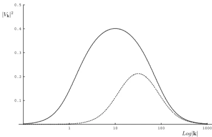
Figure 1. Fermion condensation density|Vk|2as a function
of|k|and for sample values of the parametersm1andm2.
Solid line:m1= 1,m2= 100; Long dashed line: m1= 10,
m2= 100; Short dashed line:m1= 10,m2= 1000.
whereUkandVkare Bogoliubov coefficients given by:
Vk(t) = |Vk|ei(ωk,2+ωk,1)t, (14)
Uk(t) = |Uk|ei(ωk,2−ωk,1)t, (15)
|Uk| =
µω
k,1+m1
2ωk,1
¶12µω
k,2+m2
2ωk,2
¶12
×
µ
1 + |k|
2
(ωk,1+m1)(ωk,2+m2)
¶
,
|Vk| =
µ
ωk,1+m1
2ωk,1
¶12µω
k,2+m2
2ωk,2
¶12
×
µ
|k|
(ωk,2+m2)−
|k|
(ωk,1+m1)
¶
, (16)
with
|Uk|2+|Vk|2= 1. (17)
The function|Vk|is related to the condensate content of the flavor vacuum [3] as:
e,µh0|αrk†,iαrk,i|0ie,µ = sin2θ|Vk|2, i= 1,2 (18)
with the same result for antiparticles.
In Fig.1, we plot the fermion condensation density|Vk|2
in function of |k| and for sample values of the parameters m1 andm2. |Vk|2 is zero for m1 = m2, it has a
maxi-mum at |k| = √m1m2 and, for |k| ≫
√m
1m2, it goes
like|Vk|2≃(m2−m1)
2/(4|k|2).
From the study of the current algebra, we obtain the flavor charge operators that, in terms of flavor operators, are:
Qσ(t) =
X
k,r
³
αrk†,σ(t)αr
k,σ(t)−β r†
−k,σ(t)βr−k,σ(t)
´
withσ=e, µ.
At time t = 0, the vacuum state is |0ie,µ and the one
electron neutrino state is defined as:
|νei ≡αrk†,e|0ie,µ
Considering the flavor charge operators, defined as in Eq.(19). We then have (in the Heisenberg representation)
e,µh0|Qe(t)|0ie,µ =e,µ h0|Qµ(t)|0ie,µ= 0, (20)
Qe
k,e(t) =hνe|Qe(t)|νei (21)
=¯¯ ¯ n
αrk,e(t), α r†
k,e(0)
o¯ ¯ ¯ 2 +¯¯ ¯ n
β−r†k,e(t), αrk†,e(0)o¯¯ ¯
2
,
Qe
k,µ(t) =hνe|Qµ(t)|νei (22)
=¯¯ ¯ n
αrk,µ(t), α r†
k,e(0)
o¯ ¯ ¯ 2 +¯¯ ¯ n
β−r†k,µ(t), αrk†,e(0)o¯¯ ¯
2
.
Charge conservation is obviously ensured at any time:
Qe
k,e(t) +Qek,µ(t) = 1. (23)
The oscillation formula for the flavor charges are then [8]:
Qek,e(t) = 1−sin2(2θ)
h
|Uk|2sin2
µ
ωk,2−ωk,1
2 t
¶
+ |Vk|
2
sin2
µω
k,2+ωk,1
2 t
¶ i
, (24)
Qek,µ(t) = sin2(2θ)
h
|Uk|
2
sin2
µω
k,2−ωk,1
2 t
¶
+ |Vk|2sin2
µω
k,2+ωk,1
2 t
¶i
. (25)
This result is exact. There are two differences with re-spect to the usual formula for neutrino oscillations: the am-plitudes are energy dependent, and there is an additional os-cillating term.
For|k| ≫√m1m2we have|Uk|
2
−→1and|Vk|2 −→
0and the traditional formula is recovered.
Similar results are obtained in the case of boson fields [10]. For theη−η′system, the correction may be as large as
20%.
3
Neutrino mixing contribution to the
cosmological constant
The connection between the vacuum energy density hρvaci
and the cosmological constant Λ is provided by the well known relation
hρvaci=
Λ
4πG, (26)
whereGis the gravitational constant.
The energy–momentum tensor densityTµνis obtained by
varying the action with respect to the metricgµν:
Tµν =
2
√ −g
δS
δgµν(x), (27)
where the action is S=
Z √
−gL(x)d4x. (28) In the present case, the energy momentum tensor density is given by
Tµν(x) =
i
2
³
¯
Ψm(x)γµ(x)←D→νΨm(x)
´
, (29)
where←D→νis the covariant derivative:
Dν=∂ν+Γν, Γν=
1 8ω
ab
ν [γa, γb], γµ(x) =γcecµ(x),
(30) beingγcthe standard Dirac matrices, andΨ¯←D→
νΨ = ¯ΨDΨ−
(DΨ)Ψ¯ . Let us consider the Minkowski metric, we have
T00(x) =
i
2 :
³
¯
Ψm(x)γ0←→∂ 0Ψm(x)
´
: (31) where:... :denotes the customary normal ordering with re-spect to the mass vacuum in the flat space-time.
In terms of the annihilation and creation operators of fieldsν1andν2, the energy-momentum tensor
T00=
Z
d3xT00(x) (32)
is given by T00(i)=
X
r
Z
d3kωk,i
³
αrk†,iαrk,i+β r† −k,iβ
r
−k,i
´
, (33)
withi= 1,2.
Note thatT00(i)is time independent.
The expectation value ofT00(i)in the flavor vacuum|0if
gives the contribution hρmix
vaciof the neutrino mixing to the
vacuum energy density is:
fh0|
X
i
T00(i)(0)|0if =hρmixvaciη00. (34)
Within the QFT formalism for neutrino mixing, we have
fh0|T00(i)|0if =fh0(t)|T00(i)|0(t)if (35)
for any t. We then obtain
fh0|
X
i
T00(i)(0)|0if =
X
i,r
Z
d3kωk,i
³
fh0|αrk†,iα r
k,i|0if
+ fh0|βrk†,iβrk,i|0if
´
. (36)
By using Eq.(18), we get
fh0|
X
i
T00(i)(0)|0if = 8 sin2θ
Z
d3k(ωk,1+ωk,2)|Vk|2
i.e.
hρmixvaci= 32π2sin2θ
Z K
0
dk k2(ωk,1+ωk,2)|Vk|2, (38)
where the cut-offKhas been introduced. Eq.(38) is our re-sult: it shows that the cosmological constant gets a non-zero contribution induced from the neutrino mixing [2]. Notice that such a contribution is indeed zero in the no-mixing limit when the mixing angleθ = 0and/orm1 =m2. Moreover,
the contribution is absent in the traditional phenomenological (Pontecorvo) mixing treatment.
We may try to estimate the neutrino mixing contribu-tion by making our choice for the cut-off. If we choose the cut-off proportional to the natural scale appearing in the mixing phenomenon k0 ≃ √m1m2 [3]: using K ∼ k0,
m1 = 7×10⁻³eV,m2 = 5×10⁻²eV, andsin2θ ≃0.3
[14] in Eq.(38), we obtain
hρmix
vaci= 0.43×10−47GeV4 (39)
Using Eq.(26), we are in agreement with the upper bound forΛ:
Λ∼10−56cm−2,
(40) Another possible choice is to use the electro-weak scale cut-off:K≈100GeV. We then have
hρmixvaci= 1.5×10⁻¹⁵GeV4 (41)
and
Λ∼10−24cm−2,
(42) which is, however, beyond the accepted upper bound.
In a recent paper [15], it was suggested the cut-off scale given by the sum of the two neutrino masses,K=m1+m2.
For hierarchical neutrino models, for which m2≫m1,
we have, in this case,K≫√m1m2,and thus, if we assume
that the modes near the cut–off contribute mainly to the vac-uum energy, and take into account the asymptotic properties ofVk:
|Vk|2≃
(m2−m1)2
4k2 k≫
√
m1m2 (43)
we obtain:
hρmixvaci ∼ 8πsin2θ(m2−m1)2(m2+m1)
2
×
×
µ√
2 + 1 +O
µ
m2 1
m2 2
¶¶
(44)
and then
hρmix vaci ∝sin
2θ(∆m2)2
(45) in the limitm2≫m1.
In Ref.[15], the corresponding∆m2is given by the solar
neutrino data: ∆m2 ≃10−5eV2, resulting in a contribution
of the right order.
4
Quantum fields and mixing in
ex-panding universe
In this Section we present a preliminary study of mixed fields on a time–dependent gravitational background. For simplic-ity, we consider the case of neutral scalar fields, the case of fermionic fields and neutrino oscillations will be considered elsewhere.
4.1
Free fields in expanding universe
We start by quantizing a free neutral scalar field φ in the Friedmann–Robertson–Walker (FRW) space-time with flat spatial sections, characterized by metrics of the form
ds2=gµνdxµdxν =dt2−a2(t)dx2, (46)
wherea(t)is the scale factor.
A flat FRW space-time is a conformally flat space-time. Indeed, by replacing the coordinatetby the conformal time η,
η(t) =
Z t
t0
dt
a(t), (47)
wheret0is an arbitrary constant, the line element takes the
form
ds2=a2(η)[dη2−dx2], (48) wherea(η)is the scale factor expressed through the new vari-ableη. Introducing the auxiliary fieldχ = a(η)φ, it is pos-sible to show that the evolution of a scalar fieldφin a flat FRW metric is mathematically equivalent to the dynamics of the auxiliary fieldχ in the Minkowski metric [16]. The in-formation about the influence of gravitational field onφis contained in the time-dependent massmeff(η)defined by
m2eff(η) =m2a2−
a′′
a , (49)
where the prime′denotes the derivative with respect toη.
The fieldχcan be quantized in the standard fashion by introducing the equal time commutation relations
[χ(x, η), π(y, η)] =iδ3(x−y), (50) whereπ=χ′is the canonical momentum.
The Hamiltonian of the quantum fieldχis
H(η) =1 2
Z
d3x£
π2+ (∇χ)2+m2eff(η)χ2¤
. (51)
Note that the energy of the fieldχis not conserved; this leads to the possibility of particle creation in the vacuum. The en-ergy for new particles is supplied by gravitational field.
The fieldχis expanded as
χ(x, η) =
Z d3k
(2π)32
eikx
√
2
³
vk∗(η)ak+vk(η)a†−k
´
where the mode functionsvk(η)obey the equations
v′′k+ωk2(η)vk = 0, ωk(η) =
q
k2+m2
eff(η) (53)
and satisfy the following normalization condition v′
kv∗k−vkvk′∗= 2i. (54)
We have vk(η) = v−k(η) as follows from the relation
(χk)∗=χ
−kand(ak)∗=a†k, where
χk(η) =
1
√
2
³
v∗k(η)ak+vk(η)a†−k
´
. (55)
The annihilation operators are given in terms ofχk(η)
andvk(η)by:
ak=
√
2 v
′
kχk−vkχ′k
v′
kv∗k−vkvk′∗
. (56)
Note thatakis time–independent; the commutation relations
are:
[ak, a†k′] =δ
3(k
−k′), [ak, ak′] = [a†k, a†k′] = 0. (57)
The vacuum state annihilated byakis denoted by|0(η)i:
ak|0(η)i= 0.
4.2
The instantaneous vacuum
The Hamiltonian Eq.(51) is time dependent, then we can define an “instantaneous” vacuum by selecting an arbitrary timeη0and defining the vacuum|0(η0)ias the lowest energy
eigenstate of the Hamiltonian H(η0) computed at the time
η0.
The mode functionsvk(η0), corresponding to the vacuum
|0(η0)i, are obtained by computing the expectation value
h0(η)|H(η0)|0(η)iin the vacuum state|0(η)idetermined by
arbitrary chosen mode functionsvk(η)and then minimizing
that expectation value with respect to all possible choice of vk(η)[16].
The Hamiltonian Eq.(51) expressed through the annihi-lations operatorsak defined by the arbitrary mode functions
vk(η)is
H(η) = 1 4
Z
d3kh³v′2
k(η) +ω2k(η)v2k(η)
´∗
aka−k
+ ³v′2
k(η) +ωk2(η)vk2(η)
´
a†ka†−k
+ ³|vk′(η)|2+ω2k(η)|vk(η)|2
´³
2a†kak+δ3(0)
´i
.
(58) Sinceak|0(η)i= 0, we have
h0(η)|H(η0)|0(η)i =
1 4δ
3(0)Z d3k³
|v′k(η)|2
+ ωk2(η)|vk(η)|2
´
η=η0
and the density energy is ρ= 1
4
Z
d3k³|v′
k(η)|2+ωk2(η)|vk(η)|2
´
η=η0
. (59)
At fixed value of the momentumk, ifω2
k(η0) >0, it is
possible to show that the mode functionsvk(η)that minimize
ρsatisfy the following initial conditions atη=η0[16]:
vk(η0) = p 1
ωk(η0)
, v′k(η0) =i
p
ωk(η0). (60)
The mode functions satisfying the Eq.(60) define the an-nihilation operatorsa0
kof the vacuum|0(η0)i:a0k|0(η0)i= 0
through which the HamiltonianH(η0)at timeη0is expressed
as
H(η0) =
Z
d3kωk(η0)
³
a0k†a0k+1 2δ
3(0)´.
(61)
The zero point energy density of quantum field in the vac-uum state|0(η0)iis
ρ0=
1 2
Z
d3kωk(η0). (62)
This quantity is time dependent, but, considering the prob-lem of particle oscillations in the present time, since the time scale of mixing phenomena are much smaller than the cos-mological time scale, we can neglect the particle creation in the vacuum due to the gravitational field and we may consider ρ≃constantat the present time and then we renormalize in usual way.
For further analysis of the vacuum structure in a curved background see refs.[17].
4.3
Mixed fields in expanding universe
The boson mixing relations in FRW space-time are general-ized as
χA(x, η) =χ1(x, η) cosθ+χ2(x, η) sinθ
χB(x, η) =−χ1(x, η) sinθ+χ2(x, η) cosθ(63)
We now proceed in a similar way to what has been done in Ref.[10] for bosons in flat space-time and recast Eqs.(63) into the form:
χA(x, η) =G−θ1(η)χ1(x, η)Gθ(η)
χB(x, η) =G−θ1(η)χ2(x, η)Gθ(η) (64)
and similar ones forπA(x, η),πB(x, η). Gθ(η)denotes the
operator which implements the mixing transformations (63): Gθ(η) = exp[θS(η)], (65)
with
S(η) = −i
Z
d3x³π1(x, η)χ2(x, η)
− π2(x, η)χ1(x, η)
´
We have, explicitly
S(η) =
Z
d3k³Uk∗(η)a†k,1ak,2−Vk∗(η)a−k,1ak,2
+ Vk(η)a†−k,1a
†
k,2−Uk(η)ak,1a†k,2
´
(67) whereUk(η)andVk(η)are Bogoliubov coefficients given by
Uk(η) ≡ i
£
v′∗
k,1(η)vk,2(η)−vk,2′ (η)vk,1∗ (η)
¤
, (68) Vk(η) ≡ −i£vk,1′ (η)vk,2(η)−vk,2′ (η)vk,1(η)¤.(69)
and satisfy the relation
|Uk|2− |Vk|2= 1. (70)
Similar results can be obtained in the case of fermion mixing.
4.4
The de Sitter space-time
The de Sitter space-time is characterized by a scale factor of the form
a(t)∼eHt, (71)
whereH = ˙a/a >0is the Hubble constant. The conformal timeη, the scale factora(η)and the effective frequency are given by
η=−H1e−Ht, a(η) =− 1
Hη, (72) ω2
k(η) =k2+
³m2
H2 −2
´1
η2. (73)
The conformal timeηranges from−∞to0when the proper timetgoes from−∞to∞. The origin ofηis chosen so that the infinite future corresponds toη= 0.
For this space-time, the general solution of Eq.(53) is vk(η) =
p
k|η|hAJn(k|η|) +BYn(k|η|)
i
, (74)
withn = q9 4 −
m2
H2, A and B constants, and Jn(k|η|)and
Yn(k|η|)Bessel functions.
In the de Sitter space-time, a suitable vacuum state is the Bunch-Davies vacuum, defined as the Minkowski vacuum in the early time limit (η→ −∞):
vk(η) =
1
√ω
k
eiωkη, η→ −∞. (75)
In this case, the mode functions are
vk(η) =
r
π|η|
2
h
Jn(k|η|)−iYn(k|η|)
i
, (76)
withn=q94−m2
H2.
Assuming for the present time, i.e. the actual time relative to the observer,
t= 0 ⇒ η=−1
H ⇒ a(η) = 1, (77)
the mixing transformations in the flat space-time are good approximation of those in FRW space-time Eqs.(63), since the time scale of mixing phenomena are much smaller than the cosmological time scale. The results obtained in Section III describe the contribution to the value of the cosmological constant given by the neutrino mixing at present time.
5
Conclusions
The neutrino mixing is a possible source for the cosmologi-cal constant. Indeed, the non–perturbative vacuum structure associated with neutrino mixing leads to a non–zero contribu-tion to the value of the cosmological constant [2]. The value of Λ consistent with its accepted upper bound is found by using the natural scale of the neutrino mixing cut–off. The origin of the contribution here discussed is completely differ-ent from that of the ordinary contribution to the vacuum zero energy of a massive spinor field: it is themixingphenomenon which provides the vacuum energy contribution discussed in this paper.
Acknowledgments
We thank MURST, INFN, INFM and ESF Program COSLAB for financial support.
References
[1] Ya. B. Zeldovich, I. D. Novikov,Structure and evolution of the universe(Izdatel’stvo Nauka, Moscow, 1975); V. Sahni and A. A. Starobinsky, Int. J. Mod. Phys. D9, 373 (2000).
[2] M. Blasone, A. Capolupo, S. Capozziello, S. Carloni, and G. Vitiello, Phys. Lett. A323, 182 (2004); [hep-th/0410196].
[3] M. Blasone and G. Vitiello, Annals Phys.244, 283 (1995) [Erratum-ibid.249, 363 (1995)].
[4] K. C. Hannabuss and D. C. Latimer, J. Phys. A 33, 1369 (2000); J. Phys. A36, L69 (2003).
[5] M. Binger and C. R. Ji, Phys. Rev. D60, 056005 (1999); C. R. Ji and Y. Mishchenko, Phys. Rev. D64, 076004 (2001); Phys. Rev. D65, 096015 (2002).
[6] K. Fujii, C. Habe, and T. Yabuki, Phys. Rev. D59, 113003 (1999) [Erratum-ibid. D 60 (1999) 099903]; Phys. Rev. D
64, 013011 (2001); K. Fujii, C. Habe, and M. Blasone, [hep-ph/0212076].
[7] M. Blasone and G. Vitiello, Phys. Rev. D60, 111302 (1999); M. Blasone, P. Jizba, and G. Vitiello, Phys. Lett. B517, 471 (2001);
[8] M. Blasone, P. A. Henning, and G. Vitiello, Phys. Lett. B451, 140 (1999); M. Blasone, P. P. Pacheco, and H. W. C. Tseung, Phys. Rev. D67, 073011 (2003).
[9] M. Blasone, J. Magueijo, and P. Pires-Pacheco, [hep-ph/0307205].
[11] M. Blasone, A. Capolupo, and G. Vitiello, Phys. Rev. D66, 025033 (2002).
[12] M. Blasone and J. Palmer, Phys. Rev. D69, 057301 (2004).
[13] A. Capolupo, Ph.D. thesis (2004), [hep-th 0408228];
[14] G.L. Fogli, E. Lisi, A. Marrone , A. Melchiorri, A. Palazzo, P. Serra, and J. Silk, [hep-ph/0408045].
[15] G. Barenboim and N. E. Mavromatos, [hep-ph/0406035]; N. E. Mavromatos, [gr-qc/0411067].
[16] V. F. Mukhanov, S. Winitzki,Introduction to Quantum Fields in Classical Backgrounds, Lecture notes - 2004