doi: 10.1590/0101-7438.2017.037.02.0387
QUALITY ANALYSIS FOR THE VRP SOLUTIONS USING COMPUTER VISION TECHNIQUES
Silvely S. N´eia
1*, Almir O. Artero
2and Cl´audio B. da Cunha
3Received November 25, 2016 / Accepted July 14, 2017
ABSTRACT.The Vehicle Routing Problem (VRP) is a classical problem, and when the number of cus-tomers is very large, the task of finding the optimal solution can be extremely complex. It is still necessary to find an effective way to evaluate the quality of solutions when there is no known optimal solution. This work presents a suggestion to analyze the quality of vehicle routes, based only on their geometric prop-erties. The proposed descriptors aim to be invariants in relation to the amount of customers, vehicles and the size of the covered area. Applying the methodology proposed in this work it is possible to obtain the route and, then, to evaluate the quality of solutions obtained using computer vision. Despite considering problems with different configurations for the number of customers, vehicles and service area, the results obtained with the experiments show that the proposal is useful for classifying the routes into good or bad classes. A visual analysis was performed using the Parallel Coordinates and Viz3D techniques and then a classification was performed by a Backpropagation Neural Network, which indicated an accuracy rate of 99.87%.
Keywords: Vehicle Routing Problem, Shape Analysis, Pattern Recognition.
1 INTRODUCTION
The vehicle routing problem (VRP) has important applications in many areas with different char-acteristics. The best known problem in this class is the Traveling Salesman Problem, an NP-hard problem, presented in 1934 by the mathematician Karl Menger (Garey & Johnson, 1979 [15]), which consists in finding the sequence of cities to be visited by a traveling salesman, so that all cities must be visited exactly once and the total distance traveled must be minimized. Since then, new problems and formulations have been proposed, with new necessities, including capabilities
*Corresponding author.
1Departamento de Estat´ıstica, Universidade Estadual de S˜ao Paulo, 19060-900 Presidente Prudente, SP, Brasil. E-mail: [email protected]
2Departamento de Matem´atica e Ciˆencia da Computac¸˜ao, Universidade Estadual de S˜ao Paulo, 19060-900 Presidente Prudente, SP, Brasil. E-mail: [email protected]
of vehicles, hours of operation, the maximum length of routes (time or distance), the size and composition of the fleet, the vehicle types that can meet certain customers, the precedence among customers, etc. Bodin & Golden (1981) [5], Christofides (1985) [10], Assad (1988) [3] and Ro-nen (1988) [24] and more recently by Eksioglu et al. (2009) [13] presented taxonomies, which have a more complete classification. Laporte (2009)[20], Kumar & Pannerselvam (2012) [19] and Jaegere et al. (2014) [18] provide very current surveys of the area. More recently, Miranda-Bront et al. (2015) [22] studied the swap body vehicle routing problem (SB-VRP) that is a generaliza-tion of the classical VRP.
Due to computational complexity of the issue, many methods proposed to solve this problem can be found in the scientific literature (Chaoji et al., 2008 [7]). According the taxonomy of Eksioglu et al. (2009) [13], it can be considered as cost, the travel time, the total distance traveled, the number of vehicles used, or the delay.
The VRP is an NP-hard problem, thereby if the number of costumers is too large, it is very dif-ficult to find the best solution, either by heuristic methods as exact methods. The exact methods has a computational cost usually very high. In heuristics methods, it is necessary to use a method to guarantee that the found solution will be satisfactory, that is, optimal or nearly optimal. So, it is still necessary to find an effective way to evaluate the quality of solutions when there is no known optimal solution to the problem.
This work presents a proposal to analyze the quality of vehicle routes, based only on their geo-metric shapes analysis. The other sections of this paper are organized as follows: in Section 2 are presented some works that treat the expected forms for routes in routing problems. This section shows the main shape descriptors found in the literature and evaluated in this work to analyze the routes. In this section also are presented the techniques of information visualization, used in visual analysis of data, and a technique for attributes selection, based on analysis of variance; Section 3 presents the methodology, proposed in this work, to evaluate the quality of solutions for the vehicle routing problem, based on the geometric analysis of the route shapes; In Section 4 are presented some results using the instances type “A” from Augerat et al. (1998)[4]; Finally, Section 5 presents the conclusions and future works.
2 RELATED WORKS
Cerd´a (2013) [11] present a sweep-heuristic based formulation for the VRP with cross-docking. Also in the literature, it is stand out the works of Ryan et al. (1993) [26], Vidal et al. (2014) [29] and Laporte et al. (2014) [21].
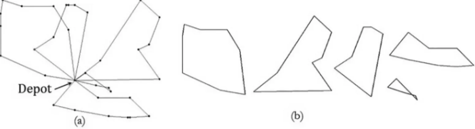
Accordingly the shape of petals seems to be one that has a good solution. Figure 1 (a) shows the routes obtained for instanceA-n33-k5, where it is observed a petal-shaped structure. In (b) shows the shapes of the five routes for this solution.
Figure 1–a) Solution for theA-n33-k5instance; b) Shape of the five routes.
2.1 Shape Analysis of Routes
Many problems in computer can be reduced to a shape analysis of images, finding important applications in many fields such as biology, medicine, visual arts and security (Takemura & Cesar Junior, 2002 [28]). However, the main difficulty is to find measures (descriptors) that are invariant to changes made by the forms, such as scale changes, rotations, translations and projections. This paper proposed and evaluated some descriptors to accomplish this task. These descriptors are described below.
Total Cost– The total cost is the total distance traveled by all vehicles.Cost Min, Cost Max
andCost Aver age, are the minimum, the maximum and the average route lengths.
Overlap– The overlap between the routes can be an indicative of bad quality of the solution found, indicating that better solutions can be obtained, combining the customers in these routes. The Figure 2 shows examples of overlap between two routes.
Perimeter – The perimeter P of a shape is defined by the sum of the length of its edges. In the case of objects in an image, can be obtained adding the distances between the pixels of its frontier, noting that the distance among pixels in the vertical and horizontal direction is 1.0 and the distance between two pixels on diagonal direction is√2. Although the perimeter may be a very simple descriptor, it has been widely used to obtain more interesting descriptors.
Area– The area of a shape Ais another descriptor very simple. In the case of a contour in an imageI, the area can be obtained by counting all pixels inside the contourICas in 1.
A=
W
i=1
H
j=1
k (1)
where:W is the image width;His the image height;k=1 if pixel(i,j)∈ ICandk=0
other-wise. In the case of a convex region, determined by itsnvertices(x1,y1), (x2,y2), . . . , (xn,yn),
the area of the convex hull is given by Equation 2.
A=(x1+x2)(y1−y2)+(x2+x3)(y2−y3)+ · · · +(xn+x1)(yn−y1) (2)
Compacity– The compacityC(Costa and Cesar (2001) [9]) is a measure defined by Equation 3, wherePis the perimeter and Ais the area of the form. The lowest compacity is obtained with a circle, which has a very large area compared to its perimeter.Compacit y Min,Compacit y Max
and Compacit y Aver age are the minimum, the maximum and the average compacity of the routes.
C= P
2
A (3)
Centroid – It is the location of the central point of the shape. From the centroid, important descriptors can be obtained, such as the minimum, maximum and average distance from the centroid to the edge. The centroid is obtained as the averages of vertices coordinates of the shape.
Diameter– The diameterDis the longest distance between any two points of the shape.
Convex Hull– The determination of the convex hull of a shape, its areaAH and its perimeterPH
are very useful to characterize shapes and also to obtain other descriptors. The convex hull of a route is the smallest convex polygon that contains the route.
Fractal Dimension– The Fractal DimensionF Dis a value that describes how irregular an object is and how much of the space it occupies. The basic principle to estimate F Dis based on the concept of self-similarity. The F D of a bounded set S in Euclidean n-space is defined as in Equation 4.
F D= lim
r→0
log(Nr)
log(n1) (4)
whereNr is the least number of copies ofSin the scaler. The union ofNr distinct copies must
an object in an image is the Box-counting method, which creates square boxes, with the image was resized to a square dimension such that the length, measured in number of pixels, was of a power of 2. This allows for the square image to be equally divided into four quadrants and each subsequent quadrant can be divided into four quadrants, and so on. The number of boxes containing black pixels was noted as a function of the box-size, length of box. The natural log of all these points were calculated and plotted and the fractal dimension will be the angular coefficient of the diagram.
Temperature– The temperatureT is a measure defined by Equation 5, where Pis the perime-ter and PH is the perimeter of the convex hull. The contour temperature is defined based on
thermodynamics formalism. The authors that proposed this feature argues that is bear strong re-lationships with the fractal dimensions (Costa & Cesar (2001) [9] and DuPain et al., 1986 [12]).
T =
log2
2P P−PH
−1
(5)
Curvature– The curvature is one of the most important descriptors that can be extracted from a contour. Given a parametric curveS(t)=(x(t),y(t)), the curvaturek(t)is defined by Equa-tion 6.
k(t)= x
′
(t)y′′(t)−x′′(t)y′(t)
x′2(t)
+y′2(t)32
(6)
Bending Energy– The bending energyB Eis obtained by integrating the squared curvature values along the contour and dividing the result by curve perimeter, as Equation 7.
B E = 1 P
k(t)2dt (7)
3 TECHNIQUES FOR MULTIDIMENSIONAL VISUALIZATION INFORMATION
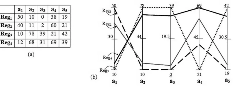
Due to the large number of descriptors used in this work, it is necessary to use information visualization techniques (Card et al., 1999 [6]) to display the high dimensional data, such as Parallel Coordinates (Inselberg, 1985 [17]), which allows visualizing all attributes in A 2D chart. In parallel coordinates, a space of dimension n is mapped to a two-dimensional space using equidistant n and parallel axes to principal axes. Each axis represents an attribute, and normally, the interval of values for each attribute is linearly mapped on the corresponding axis. Each data item is showed as a polygonal line that intercepts each axis at the point corresponding to the value of the associated attribute, as shown in Figure 3.
Each axis is labeled with the name, the lowest and highest value of each attribute, and the inter-pretation is facilitated by the immediate estimation of the attribute values along the axes. Other structures can be identified, such as data distribution and functional dependencies, correlations between attributes (Wegman & Luo, 1996 [30]) and clusters.
cylin-Figure 3–a) Set of data with four records of dimension five, b) Visualization using parallel coordinates of the set showed in (a).
der, whose base consists in system of radial axes which represent the attributes of the records. Given the data matrixDm×n, the Viz3D maps the n-dimensional coordinates of m records di of
D in 3D coordinates(xi,yi,zi)according to Equation 8.
xi =xC+n1nj=1
di,j−minj
maxj−minjcos
2πj n
yi =yC+1n
n j=1
di,j−minj
maxj−minjsin
2πj n
zi =zC+n1nj=1
di,j−minj
maxj−minj
(8)
with: i = 1, . . . ,n; j =1, . . . ,m; (xc,yc,zc)is the origin of the 3D radial system;maxj =
maximum(dk,j)andminj =minimum(dk,j), fork=1, . . . ,m.
Figure 4 illustrates the Viz3D projection and Artero and Oliveira (2004)[1] argue that the views obtained with this projection are similar to those obtained using Principal Component Analysis (PCA) when used to reduce dimensionality of data to the dimensional of the space.
4 ATTRIBUTES SELECTION
Figure 4–Projection in the Viz3D (Artero and Oliveira, 2004[1]).
a sample ofk(classes) groups, withn registers, the critical value of SnedecorF is determined by Equation 9.
F =
c
j=1nj(x¯j− ¯x)2(n−k)
c j=1
nj
i=1(xi,j − ¯xj)2(k−1)
(9)
where:cis the number of class j;n is the total number of samples in the set;nj is the number
of samples in the class j;x¯jis the mean of samples in class j;x¯is the mean of all samples in the
data set;kis the degree freedom;xi,j is the samplei in the class j.
When the calculated value ofFis greater than the critical value in the Snedecor distribution, the analyzed attribute is considered relevant for separating classes and therefore should be retained in the analysis.
5 ANALYSIS OF SOLUTIONS FOR VEHICLE ROUTING PROBLEM USING
TECHNIQUES OF COMPUTATIONAL GEOMETRY
The total cost of the solution is an obvious indicator on the quality of the route, however, only an-alyzing this attribute is not possible to classify the solution as good or bad, because for problems with multiple nodes (costumers) to be serviced is natural that the total cost is high, even for the optimal solution, since the total cost depends on the area covered by us. Two simples possibilities to evaluate the quality of a solution, independent of the quantity and area covered by the nodes, would be the ratiosQ1andQ2, given in Equations 10 and 11, which are two new attributes.
Q1= Cost T ot al
ConvH ull Ar ea (10)
Q2=
T emperat ure
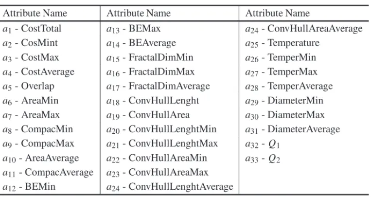
In this work, we propose that the descriptors presented in Subsection 2.1 and descriptors in Equations 10 and 11 may be applied to assess the quality of the solutions to the vehicle routing problem by means of a geometrical analysis of routes. These descriptors are applied individually to the routes traveled by the vehicle, and total path traveled by all vehicles in this manner, the descriptors are predicted minimum, maximum and average of each solution, yielding a total of 34 attributes in the next Table 1.
Table 1–Attribute Names.
Attribute Name Attribute Name Attribute Name
a1- CostTotal a13- BEMax a24- ConvHullAreaAverage a2- CosMint a14- BEAverage a25- Temperature
a3- CostMax a15- FractalDimMin a26- TemperMin
a4- CostAverage a16- FractalDimMax a27- TemperMax a5- Overlap a17- FractalDimAverage a28- TemperAverage
a6- AreaMin a18- ConvHullLenght a29- DiameterMin
a7- AreaMax a19- ConvHullArea a30- DiameterMax a8- CompacMin a20- ConvHullLenghtMin a31- DiameterAverage
a9- CompacMax a21- ConvHullLenghtMax a32-Q1 a10- AreaAverage a22- ConvHullAreaMin a33-Q2 a11- CompacAverage a23- ConvHullAreaMax
a12- BEMin a24- ConvHullLenghtAverage
In addition to these attributes, the records (solutions) also receive, according to the cost of the solution (sum of the solution routes) a last attribute corresponding to Class 1 for good routes and Class 2 for bad. Figure 5 shows the ideal solution and a poor solution for instanceA-n36-k5, which is small andA-n80-k10, which is large.
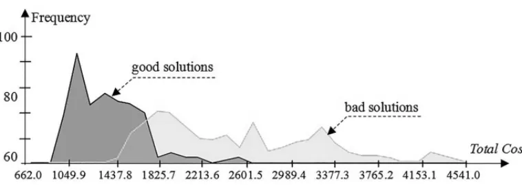
Looking at Figure 6, which shows the distribution of total costs in classes good and bad, it is observed that the total cost of the optimal solution instanceA-n80-k10is often greater than the total cost of bad solution in the instanceA-n33-k5, showing that the total cost is not a useful measure to separate the good and bad solutions.
Figure 5– Solutions for the instanceA-n33-k5: a) Optimal (total cost = 662.76); b) Poor (total cost = 1,522.10). Solutions for the instanceA-n80-k10: c) Optimal (total cost = 1,766.50); d) Poor (total cost = 4,539.76).
Figure 6–Distribution of attribute values CostTotal for the classes good and bad.
6 EXPERIMENTS
A-n45-k7, A-n46-k7, A-n48-k7, A-n53-k7, A-n54-k7, A-n55-k9, A-n60-k9, A-n61-k9, A-n62-k8, A-n63-k9, A-n63-k10, A-n64-k9, A-n65-k9, A-n69-k9andA-n80-k10. The study was constructed generating 70 solutions for each one of the 27 instances of Augerat et al. (1998) [4], (accumulat-ing 1,890 solutions), us(accumulat-ing the Clarke and Wright heuristics (Clark & Wright, 1964 [8]), and then the 15 best solutions and the 15 worst solutions we selected, were adopted 405 good solutions (total cost low) and 405 bad (high total cost), resulting in 15 good and 15 bad solutions for each one of the 27 instances, always considered the capacity maximum limit vehicle.
6.1 Visual Data Analysis
The visualization in parallel coordinates of all the attributes is shown in Figure 7, where the polygonal matching to the good solutions are presented in black, while the polygonal matching to the bad solutions are displayed in gray.
Figure 7–Parallel Coordinates Visualization of the 34 attributes (descriptors). Black polylines for the 405 good solutions and gray polylines for the 405 bad solutions.
Sorting the axes with the values of F-Snedecor it is easy to identify the most relevant attributes for the separation of the two classes, as illustrated in Figure 8.
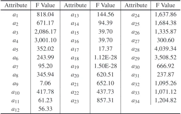
TheFvalues for these 34 attributes are shown in Table 2.
Table 2–Values of F for the 34 attributes (descriptors) a1, a2,. . . ,a34.
Attribute F Value Attribute F Value Attribute F Value
a1 818.04 a13 144.56 a24 1,637.86
a2 671.17 a14 94.39 a25 1,684.38 a3 2,086.17 a15 39.70 a26 1,335.87
a4 3,001.10 a16 39.70 a27 300.60
a5 352.02 a17 17.37 a28 4,039.34 a6 243.99 a18 1.12E-28 a29 3,508.52
a7 95.20 a19 1.50E-28 a30 666.92
a8 345.94 a20 620.51 a31 237.87
a9 7.06 a21 652.10 a32 1,095.26
a10 417.78 a22 437.73 a33 1,071.12
a11 61.23 a23 857.31 a34 1,204.82 a12 56.33
The ten attributes with the higher values (better) of theFof Snedecor, all above than 1,000 are shown in Table 3.
Table 3–Attributes with the 10 higher values (best) ofF.
Attribute Attribute Name F Value
a28 TemperMax 4,039.34
a29 TemperAverage 3,508.52
a4 CostAverage 3,001.10
a3 CostMax 2,086.17
a25 ConvHullAreaAverage 1,684.38
a24 ConvHullLenghtAverage 1,637.86
a26 TemperTotal 1,335.87
a34 Q2 1,204.82
a32 DiameterAverage 1,095.26
a33 Q1 1,071.12
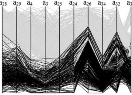
The visualization, using parallel coordinates, of the 10 attributes with the highest values (best values) of F is shown in Figure 9. In this view, it is clear that there is a good separation between the two classes, with lower values for these attributes in Class of good solutions and higher values in the class of bad solutions.
Figure 9–Visualization in parallel coordinates of the records good and bad, using only the 10 attributes with the highest values of F. Black polylines for the 405 good solutions and gray polylines for the 405 bad
solutions.
The visualization of these registers in Viz3D is shown in Figure 10, where it is possible to observe a reasonable separation between the markers in the two classes (good solutions in black and bad solutions in gray).
It is noted that four of ten attributes are obtained from the temperature information, which in-dicates that this measure can be very useful to obtain a reasonable attribute to distinguish good from bad solutions routing solutions for the problem of routing.
Figure 10–Viz3DVisualization of the records good and bad, using only the 10 attributes with the highest values of F. Black markers for the 405 good solutions and gray markers for the 405 bad solutions.
The distribution of the values in the two classes for the attribute with the highest value F
(T emper Max) (maximum temperature) is presented in Figure 11, which indicates a better separation between the two classes (Good solutions,T emper Max <0.38 and bad solutions,
Figure 11–Distribution of the attribute valuesTemperMaxin the two classes good and bad. Black color for the 405 good solutions and gray color for the 405 bad solutions.
Using theT emper Max attribute, it is possible to see in Figure 12 that regardless of the number of customers in the instances and the size of the area covered by the customers, the classes have a good separation regardless of the number of nodes (customers).
Figure 12–Good (Black) and Bad (Gray) solutions.
As the optimal costs of instances of Augerat et al. (1998) [4] are known, it is possible to deter-mine an optimality index of other solutions obtained for these instances, given by the relation in 12.
O pt imalit y = Total Solution Cost
Optimal Solution Cost (12)
the Optimality values are presented in Table 4. Again, the attributes obtained from the tempera-ture appear among the best.
Table 4–The six attributes with the highest correlation with the Optimality.
Attribute Attribute Name Correlation with the Optimality
a28 TemperMax 0.944
a29 TemperAverage 0.942
a25 ConvHullAreaAverage 0.860
a34 Q2 0.857
a32 ConvHullLenghtAverage 0.844
a33 Q1 0.834
6.2 Classification using a Neural Network Backpropagation
Using a backpropagation neural network (Rumelhart et al., 1986 [25]; Artero, 2009 [2]), this section presents the results of a classification using the same 10 previously selected attributes, aiming to evaluate the effectiveness of these ten attributes with higher values of F, to classify Solutions as good or bad. The neural network used has ten neurons in the input layer; Five in the dark and two on the way out. Logistics transfer function and learning rate 0.5 was adopted (Rumelhart et al., 1986 [25], Artero, 2009 [2]). After 2,000 training iterations, consuming a time of only four seconds, the maximum error of the network was 3.19E-14, indicating a great convergence of the network, resulting in a success rate of 99.87% (809 hits). The confusion matrix obtained by classification using the neural network is presented in Equation 13.
C M =
405 1 0 404
(13)
7 CONCLUSIONS
It is not a simple task to find optimal solutions to the vehicle routing problem, when there are a large number of customers and vehicles, as well as different sizes and shapes of the assisted areas. Heuristic methods can obtain solutions in an acceptable time, however, when the optimal solution is unknown, it is hard to discern how good is the solution with respect to the optimality, without running lower bound methods.
de-scriptor TemperMax (maximum temperature) stood out in the discrimination of the two classes (Figure 11), as well as other temperature changes. In future works, other descriptors need to be evaluated, for example, descriptors based on moments, Fourier, etc.
REFERENCES
[1] ARTEROAO & OLIVEIRAMCF. 2004. Viz3D: Effective Exploratory Visualization of Large Multi-dimensional Data Sets. In:Proc. of the Computer Graphics and Image Processing Symposium,Vol.? 340–347.
[2] ARTEROAO. 2009. Inteligˆencia Artificial – Te ´orica e Pr´atica. S˜ao Paulo: Editora Livraria da F´ısica.
[3] ASSADAA. 1988. Modeling and implementation issues in vehicle routing. In: GOLDENB & ASSAD AA (Eds). Vehicle Routing: methods and studies, North-Holland, Amsterdam, Elsevier Sciencies Publishers, pp. 7–45.
[4] AUGERATP, BELENGUERJ, BENAVENTE, CORBERAN´ A & NADDEFD. 1998. Separating capacity constraints in the CVRP using tabu search.European Journal of Operations Research,106(2,3): 546– 557.
[5] BODINLD & GOLDENB. 1981. Classification in vehicle routing and scheduling.Networks,11(2): 97–108.
[6] CARD SK, MACKINLAYJD & SHNEIDERMANB. 1999. Readings in Information Visualization, Using Vision to Think. Morgan Kaufmann.
[7] CHAOJIV, HASANMA, SALEMS, BESSONJ & ZAKIMJ. 2008. ORIGAMI: A novel and effective approach for mining representative orthogonal graph patterns.Statistical Analysis and Data Mining, 1(2): 67–84.
[8] CLARKEG & WRIGHTJW. 1964. Scheduling of vehicles from a depot to a number of delivery points.Operations Research,12(4): 568–581.
[9] COSTALF & CESARJRRM. 2001. Shape Analysis and Classification. Boca Raton: CRC Press.
[10] CHRISTOFIDESN. 1985. Vehicle routing. In: LAWEREL, LENSTRAJK, RINNOOYKANAHG & SHMOYSDB (Eds.). The Traveling Salesman Problem: A Guided Tour of Combinatorial Optimiza-tion, J. Wiley & Sons, pp. 431–448.
[11] DONDOR & CERDA´ J. 2013. A sweep-heuristic based formulation for the vehicle routing problem with cross-docking.Computers and Chemical Engineering,48: 293–311.
[12] DUPAINY, KAMAET & MENDES` FRANCEM. 1986. Can One Measure the Temperature of a Curve? Arch. Rational Mech. Anal.,94(2): 155–163.
[13] EKSIOGLUB, VURALAV & REISMANA. 2009. The vehicle routing problem: A taxonomic review. Computers & Industrial Engineering,57(4): 1472–1483.
[14] FOSTERBA & RYANDM. 1976. An Integer Programming Approach to the Vehicle Scheduling Problem.Operational Research Quarterly,27(2): 367–384.
[15] GAREYMR & JOHNSONDS. 1979. Computers and Intractability: A Guide to the Theory of NP Completeness. W.H. Freeman.
[17] INSELBERGA. 1985. The Plane with Parallel Coordinates,The Visual Computer,1(2): 69–91.
[18] JAEGEREND, DEFRAEYEM & NIEUWENHUYSEIV. 2014. The vehicle routing problem: state of the art classification and review. FEB Research Report KBI1415, Leuven, Belgium.
[19] KUMARSN & PANNEERSELVAMR. 2012. A Survey on the Vehicle Routing Problem and Its Vari-ants.Intelligent Information Management,4: 66–74.
[20] LAPORTEG. 2009. Fifty Years of Vehicle Routing,Transportation Science,43(4): 408–416.
[21] LAPORTEG, ROPKES & VIDALT. 2014. Heuristics for the vehicle routing problem. In: TOTH P & VIGOD (Eds.). Vehicle routing: Problems, methods and applications, MOS-SIAM series in optimization, Philadelphia, pp. 87–116.
[22] MIRANDA-BRONTJJ, CURCIOB, M ´ENDEZ-D´IAZI, MONTEROA, POUSAF & ZABALAP. 2012. A cluster-first route-second approach for the Swap Body Vehicle Routing Problem.Annals of Opera-tions Research,253(2): 935–956.
[23] RENAUDJ, BOCTORFF & LAPORTEG. 1996. An Improved Petal Heuristic for the Vehicle Routeing Problem.Journal of the Operational Research Society,47: 329–336.
[24] RONEND. 1988. Perspectives on practical aspects of truck routing and scheduling.European Journal of Operational Research,35(2): 137–145.
[25] RUMELHART DE, HINTON GE & WILLIAMS RJ. 1996. Learning representations by back-propagating errors.Nature,323(6088): 533–536.
[26] RYANDM, HJORRINGC & GLOVERF. 1993. Extension of the petal method for vehicle routing. Journal of Operational Research Society.,44: 289–296.
[27] SNEDECORGW & COCHRANWG. 1967. Statistical Methods (7th ed.): Iowa State.
[28] TAKEMURACM & CESARJR RM. 2002. Shape Analysis and Classification using Landmarks: Polygonal Wavelet Transform. In: Proc. 15th European Conference on Artificial Intelligence ECAI2002., 726–730.
[29] VIDALT, CRAINICTG, GENDREAUM & PRINSC. 2014. Implicit depot assignments and rotarions in vehicle routing heuristics.European Journal of Operational Research.,237(1): 15–28.
[30] WEGMAN & LUO. 1996. Implicit depot assignments and rotations in vehicle routing heuristics.
![Figure 4 – Projection in the Viz3D (Artero and Oliveira, 2004[1]).](https://thumb-eu.123doks.com/thumbv2/123dok_br/18871440.420200/7.1063.335.793.158.474/figure-projection-viz-d-artero-oliveira.webp)