This paper presents a numerical analysis of prestressed hollow core slabs under long term loading. The model considers the time dependence of material and rheological properties in order to predict the actual stage of displacements, strains and stresses. It also takes into account load changes. For the analysis, each slab is divided in a inite number of bar elements, in which the cross section is described in concrete elements, parallel to the lexural axis, and prestressed steel elements. For the results evaluation, the effective concrete area is considered. The numerical results are compared with experimental tests performed on two series of prestressed hollow core slabs. Each series had a different geometry, rate and distribution of prestressing strands. Mid-span displacements were evaluated up to 127 days after initial loading. Good correlation was achieved with both series at and below the service load level.
Keywords: numerical analysis, prestressed concrete, hollow core slabs, long term loading.
Este artigo apresenta os resultados de uma análise numérica de lajes alveolares protendidas extrudadas submetidas a carregamentos de longa duração. O modelo numérico considera os efeitos do tempo nas propriedades mecânicas dos materiais bem como nas propriedades reológicas, de modo a prever lechas, deformações e tensões. O modelo leva em conta também variações no carregamento. Para a análise, cada laje é sub -dividida em um número inito de elementos de barra cuja seção transversal é discretizada em elementos de concreto paralelos ao eixo de lexão, e elementos de armadura passiva. Para avaliação dos resultados é considerada a área líquida de concreto. Os resultados do modelo numérico foram comparados com valores medidos em ensaios de duas séries distintas de lajes alveolares protendidas. Cada série de lajes possuía dife -rentes geometrias, taxa e distribuição de cordoalhas. Deslocamentos no meio do vão de cada laje foram avaliados até a idade de 127 dias após o carregamento inicial. Boa correlação foi obtida com o modelo numérico para cargas menores ou iguais as de serviço.
Palavras-chave: análise numérica, lajes alveolares protendidas, carregamentos de longa duração.
Numerical analysis of prestressed hollow core slabs
under long term loading
Análise numérica de lajes alveolares protendidas
submetidas a carregamentos de longa duração
S. R. PEREIRA a [email protected]
J. M. CALIXTO a [email protected] T. P. BORTONE a [email protected]
a Escola de Engenharia - Universidade Federal de Minas Gerais. Belo Horizonte, MG. Brasil 31270-090
Received: 24 Feb 2013 • Accepted: 23 Jul 2013 • Available Online: 12 Aug 2013
Abstract
1. Introduction
A hollow core slab is a precast, prestressing concrete member with con-tinuous voids provided to reduce weight and cost. They are primarily used as a loor deck system in residential and commercial buildings as well as in parking structures because they are economical, have good ire resistance and sound insulation properties, and are capable of spanning long distances with relatively small depths. Hollow core slabs can make use of prestressing strands, which allow slabs with depths between 150 and 260 mm to span over 9 meters.
When used in buildings, several hollow core slabs are placed next to each other to form a continuous loor system. The small gap that is left between each slab is usually illed with a non-shrink grout. To give the loor a smooth inished surface, a topping slab overlay is poured on the top surface of the hollow core slabs. This topping slab is typically 5 cm deep. The voids in a hollow core slab may be used for electrical or me-chanical runs. For example, routing of a lighting circuit through the cores can allow ixtures in an exposed slab ceiling without unsightly surface mounted conduit.
Structurally, a hollow core slab provides the eficiency of a prestressed member for load capacity, span range, and delection control. In addition, a basic diaphragm is provided for resisting lateral loads by the grouted slab assembly provided proper connections and details exist (PCI [1]). The basic manufacturing method currently in use for the production of hollow core slabs is a dry cast or extrusion system where a very low slump concrete is forced through the machine. The cores are formed with augers or tubes with the concrete being compacted around the cores. In this scenario, the objective of this paper is to present a numerical analy -sis of prestressed hollow core slabs under long term loading. The model-ling considers not only the load history of hollow core slabs but also the effects of time in the mechanical properties of the concrete. The slabs are divided in a number of elements each having different material proper-ties as well as load histories. The results of the numerical analysis are compared to experimental tests performed on two series of prestressed hollow core slabs. Each series had a different geometry and rate and distribution of strands as well as material properties. Loads and mid-span displacements were evaluated up to 127 days after initial loading.
2. The numerical model
2.1 Assumptions
In the development of the numerical modelling [2], the following assumptions are introduced:
1. The hollow core slab, the applied loads and the deformations lie in a plane; the plane of loads is a plane of symmetry for the slab. 2. The slab is slender, that is, its length is much larger than its
lateral dimensions.
3. Transverse and longitudinal displacements are ininitesimal. 4. Only normal strains parallel to the axis of the slab are considered. 5. The geometry of the slab can vary with respect to time as well
along the length.
6. The material properties, in each section, can be different in each element.
7. The effect of shrinkage, creep and cracking as well as the evo-lution of the mechanical properties of the concrete with time are taken into account.
8. The losses due to steel relaxation in the strands are also considered.
9. The applied loads vary along time.
2.2 Formulation
In the derivation of the model, the slab is divided in a number of sections, each of one composed of elements. These elements can have different geometrical and material properties as well load his-tories. It is assumed that at a generic time tu the total strain in a concrete element i is known and given by:
(1)
( )
( )
( ) ( )
cs[
s( ) ( )
u s s]
t
t c28
u c 0 u
ci
t
t,
E
1
E
t
,
d
d
d
t
t
u 0
b
b
e
t
t
t
s
t
j
t
e
+
-÷÷ø
ö
ççè
æ
+
=
ò
¥The total strain in this case includes the effects of the applied loads as well creep and shrinkage. These effects correspond to the irst, second and third terms respectively of the right hand side in the equation above. The expression for the shrinkage strain and creep coeficient as well as the concrete tangent modulus of elasticity at time τ are the ones presented in NBR 6118 [3]. If a generic time in -terval (tu+1 – t0) is divided in a number of time steps, the total strain of each concrete element i in each section of the slab becomes:
(2)
( )
(
) ( )
( ) ( ) ( )
ci j j1u
1
j c28
1 j 1 u j 1 u 1 j c j c 0 1 u
ci
E
t
t,
t,
t
t,
t
t
E
1
t
E
1
2
1
t,
t
-= -+ +-+
å
÷
÷
ø
ö
ç
ç
è
æ
+
+
+
=
j
j
sD
e
( ) ( )
(
) ( ) ( )
ci u1 u u1
j c28
u 1 u 1 u 1 u u c 1 u
c
E
t
t,
t,
t
t,
t
t
E
1
t
E
1
2
1
+ = + + + +å
ççè
æ
+
+
+
÷÷ø
ö
+
j
j
sD
( ) ( )
[
s u1 s s]
cs
b
t
b
t
e
-+
¥ +From equation (2) it can be seen that each concrete element can have different material and load history at every time step. It is important to point out that the creep effects are considered to the time step (tu+1) and ϕ
(
tu+1,tu+1)
=0.In equation (2) the incremental stress in each concrete element
∆σci (tu+1,tu) can be explicitly determined if one rewrites the equation
after splitting the second summation. Thus:
(3)
( )
[
( ) ( )
]
÷÷
ø
ö
çç
è
æ
+
+
-=
+ + + ¥ + + 28 c u 1 u u c 1 u c s s 1 u s cs 0 1 u ci u 1 u ciE
)
t,
t(
)
t(
E
1
)
t(
E
1
2
1
t
t
)
t,
t(
t,
t
j
b
b
e
e
s
D
÷÷
ø
ö
çç
è
æ
+
+
÷
÷
ø
ö
ç
ç
è
æ
+
+
+
-+ + = -+ +-å
28 c u 1 u u c 1 u c u 1j c28 ci j j1
with
0 pri r 0
pri
t
t,
x
D
s
t
t,
s
D
=
W
x
( 6.7 5.32)r
=
e
- +)
t
(
0 pi ) r s c ( pi pris
s
D
s
D
W
=
-
+ +; if
W
<
0
, adopt
W
=
0
In this case, Dspi(c+s+r) should be determined by iterative pro-cess. For the irst attempt, consider ξr=1.
Then, the stress and strain at a strand element i at time tu+1are given by:
(9)
(
t
u 1t,
p)
E
s pit(
u 1t,
p)
pi(c s r)t(
u 1t,
p)
pi +
=
e
++
D
s
+ + +s
(10)
(
u 1 p)
pi(
u 1 p)
spi
t
+t,
= s
t
+,
t
/
E
e
For each strand element i, the maximum tensile stress is equal to
the steel yield strength.
The internal axial force and bending moment in each cross section are determined as follows:
(11)
( )
å
( )
å
( )
= + = + +
=
+
c 1 i p 1i pi u 1 p pi pi
ci 0 1 u ci 0 1 u
R
t
t,
t
t,
A
t
t,
cos(
)
A
N
s
s
a
(12)
( ) ( )
å
å
( )
= + = + +
=
+
c 1 i p 1i pi u1 p pi pi pi ci ci 0 1 u ci 0 1 u
R
t
t,
t
t,
y
A
t
t,
cos(
y)
A
M
s
s
a
The equilibrium between external and internal forces in every cross-section of the hollow core slab is given by:
(13)
EXT RN
N
=
(14)
EXT RM
M
=
The correct state of strain and the corresponding equilibrium posi -tion of the slab at each time step are obtained when both equa -tions (13) and (14) are satisied at every cross-section. If this is With this incremental stress, the inal stress in each concrete ele
-ment at time tu+1 can be obtained as:
(4)
( )
å
+(
)
=
-+
=
1 u
1
j ci j j 1
1 u
ci
t
D
s
t
t,
s
D
This final stress, in each time step, has to be compared to the concrete strength. For case of concrete in tension the limit is defined by the concrete tensile strength fctm. If this ten-sile strength is exceeded, the contribution of this element is neglected.
For the stress evaluation in each element of a prestressed strand is necessary to compute the losses of stress due to the combination of the concrete shrinkage and creep effects as well as the steel relaxation. According to Trevino and Ghali [4], the stress loss due to the steel relaxation in a strand element i is given by:
(5)
days
41
)
t
t(
0
for
1
240
t
t
ln
16
1
)
t,t
(
0 0pr 0
pri
ú
£
-
£
û
ù
ê
ë
é
÷÷ø
ö
ççè
æ
-
+
=
D
s
¥s
D
(6)
days
10
12
)
t
t(
41
for
10
12
t
t
)
t,t
(
6 0 2, 0 6 0 pr 0pri
£
-
£
´
ú
ú
û
ù
ê
ê
ë
é
÷÷ø
ö
ççè
æ
´
-=
D
s
¥sD
(7)
days
10
12
)
t
t(
for
)
t,
t(
6 0 pr 0pri
=
D
s
¥-
>
´
s
D
where:4
.
0
for
)
4
.
0
(
f
ptk 2pr¥
=
-
h
¥l
-
l
³
s
D
s
pr¥=
0
for
l
<
0
.
4
D
ptk 0 pi
f
)
t
(
s
l =
¥
=
2
.
0
for
normal
relaxation
steel
h
steel
relaxation
low
for
5
.
1
=
¥h
Thus, the stress loss in a strand element i including the concrete shrinkage and creep effects can be evaluated by:
(8)
( )
0[
cci( )
0 csi( )
0]
s pri ) r s c (pi
D
s
t
t,
e
t
t,
e
t
t,
E
s
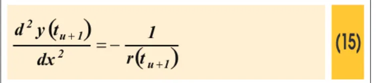
relationship is given by:
(15)
( )
( )
u 1 21 u 2
t
r
1
dx
t
y
d
+ +
=
-The rotations are obtained by integrating the above equation. Thus:
(16)
( ) ( )
ò
( )
+ +
+
=
+
x
x u 1
1 u 1 1 u
1
dx
t
r
1
t
t
q
q
not achieved a new strain state is introduced and the procedure is repeated.To ensure convergence of the iterative search process for the state of strain which satisies the equations (13) and (14), one must con -sider the compressive strength of concrete and steel stress unlim-ited. The value of these stresses should be checked at the end of the analysis. Stresses levels above usual values for service state level indicate insuficient cross-section dimensions.
After the equilibrium conditions are satisied at each cross section, the hollow core slab delected shape can be determined. With the strain of each concrete (equation 2) and strand (equation 10) ele -ment in every section, the curvature in each section along the slab is calculated. In this case the transverse displacement curvature
Figure 1 – Details of the slabs cross-sections
Series 1
A
Series 2
The transverse displacements are calculated then by:
(17)
( ) ( ) ( )
t
y
t
t
(
x
x
)
( )
t
1
dx
y
xx u 1
1 u 1 1 u 1 1 u
1
ò
+
+
-+
=
+ ++
q
q
Since each slab has been divided in sections and considering the number of the irst section equal to 1, the above equation is re -placed by:
(18)
( ) ( )
( )
( ) ( )
( )
ú
ú
û
ù
ê
ê
ë
é
-÷
÷
ø
ö
ç
ç
è
æ
+
-+
=
+ + +
+
+
)
y
t
t
x
x
1
4
r
t
1
r
t
1
i2
1
t(
y
1 u i 1 u 1 2 1 1 u 1 1 u 1 1 u
i
q
D
( )
( )
ú
ú
û
ù
ê
ê
ë
é
+
-
å
å
å
-= +
-=
-= +
1 j
1 k k u1 1 i
1 j 1 i
1 j j u1 2
t
r
1
t
r
1
2
1
D
It is important to point out that equation (18) has to satisfy the slab cinematic conditions.
3. Experimental program
In order to verify the numerical model an experimental program was carried on. It consisted on the testing of two series of hol-low core slabs. Each series had three specimens. In series 1, the hollow core slabs were 1245 mm in width and 260 mm in depth with constant hollow cores of 199 mm in diameter. They were 10 m long and pre-tensioned with 4 seven-wire low relax -ation strands (12.7 mm in nominal diameter) and 6 seven-wire low relaxation strands (11.1 mm in nominal diameter). Both strands were placed with a 30 mm bottom cover. Slabs of se-ries 2 had the same width and length as of sese-ries 1 but with a total depth of 210 mm; the hollow cores were 152 mm in diameter. They had 8 seven-wire low relaxation strands of 12.7 mm in nominal diameter placed with a 30 mm bottom cover. Both series were pre-tensioned to 75% of the ultimate strength fpu = 1900 MPa, before the concrete was cast using dry mix extrusion procedures. The applied prestressing force was transferred to the concrete 20 hours after casting. The details of the slabs cross-sections are shown in figure 1.
The concrete was produced using Brazilian type V cement and limestone as coarse aggregate. Its concrete compressive strength was evaluated employing the impact hammer. The im-pact hammer is a practical method for determining the concrete strength of slabs cast using dry mix extrusion procedures and considerably more precise than test cylinders. This is because the compaction of the machine cannot be accurately duplicated in making the cylinders. The concrete strength was evaluated at the age of 30 days for slabs of series 1 and 35 days for series 2. These ages correspond to the initial testing time in which a uniform distributed live load was applied to each slab. The av-erage concrete compressive strength at this age was 40.6 and 28.3 MPa for series 1 and 2 respectively. Both of these values correspond to an average of 9 readings taken with the impact hammer in the horizontal position on the side of each slab. The correlation to compressive cylinder strengths was made with the
use of curves printed on a plate attached to the instrument. This compressive strength was the only concrete mechanical prop-erty measured throughout the study.
The hollow core slab tests were conducted in an open area at Precon Industrial in Pedro Leopoldo, Minas Gerais. The test set-up is shown in figure 2. The specimens were subjected to a uniformly distributed load on a simple span. The clear span between the supports was 9.9 m Cement bags, with a nominal weight of 0.5 kN each, were used for the uniformly distributed load (figure 2b). A dial-gage placed at mid-span was used to measure the deflection.
The uniform distributed live load was applied incrementally af-ter each slab had been placed over supports. During the first four days, loads were incrementally applied daily. Each live load increment corresponded to 1.52 and 1.01 kN/m for series 1 and 2 respectively. These loads were kept for approximately 114 days. After that period additional loads were applied up to each slab series service live load (8.875 and 6.65 kN/m for se-ries 1 and 2 respectively). Before each live load increment and during the period of 127 days, mid-span deflections were mea-sured. These readings were always taken early in the morning to avoid temperature effects.
The temperature and relative humidity were measured daily (also early in the morning) during the testing period. Their average values were calculated and correspond to 25°C and 40% respectively.
Figure 2 – Details of the test set-up
q (kN/m)
9.9 m
Test set-up
Detail of the live load scheme
A
4. Comparative study
A comparison of the numerical and experimental results is present -ed herein. The mid-span delection for each series was select-ed for this study since it represents the overall behavior the hollow core slabs. It is important to point out that the comparison is carried out during a 4-month loading period in which the values of the loads were at or below service level.
In the numerical model, the concrete properties including shrinkage and creep effects were derived from the compressive strength mea-sured at the initial testing time and from the temperature and rela-tive humidity average values shown before. For a proper evaluation of the needed parameters, the formulation prescribed in NBR 6118 sections 8.2.8, 12.3.3, A.2.2.3 and A.2.3.2 was used. For each slab,
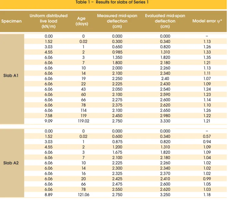
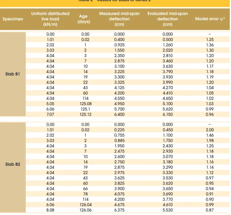
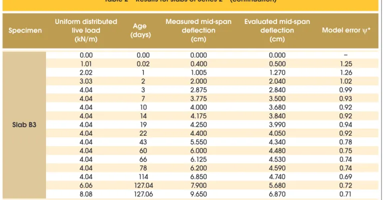
10 cross-sections along the span were analyzed at each time step with 50 concrete elements in every cross-section. The number of strand elements in every cross-section corresponded to the number of strands for each slab series: 10 for series 1 and 8 for series 2. The results of the comparative study are presented both in tabu-lar and graphical form. Table 1 shows the results for slabs of Se-ries 1 while the values correspondent to slabs of SeSe-ries 2 are in table 2. The comparison between the actual and predicted overall behavior can be quantiied based on the model error y deined as the ratio between the evaluated mid-span delection and the measured value. Values of y (last columns of tables 1 and 2) smaller than the unity indicate a stiffer behavior predicted by the numerical model. Each graph, on the other hand, shows an overall visual comparison. The comparative study for slabs of Series 1 is well represented in igure 3 which shows the load versus the midspan delection
Table 1 – Results for slabs of Series 1
Specimen
Slab A1
Slab A2
Uniform distributed
live load
(kN/m)
Age
(days)
Measured mid-span
deflection
(cm)
Evaluated mid-span
deflection
(cm)
Model error
y
*
0.00
1.52
3.03
4.55
6.06
6.06
6.06
6.06
6.06
6.06
6.06
6.06
6.06
6.06
6.06
7.58
9.09
0.00
1.52
3.03
4.55
6.06
6.06
6.06
6.06
6.06
6.06
6.06
6.06
8.89
–
1.13
1.26
1.33
1.35
1.21
1.13
1.11
1.07
1.09
1.24
1.23
1.14
1.10
1.26
1.22
1.21
–
0.57
0.94
1.09
1.09
1.04
1.02
1.02
1.02
0.99
1.05
1.03
1.18
0
0.02
1
2
3
7
10
14
19
22
43
60
66
78
114
119
119.02
0
0.02
1
2
3
7
10
14
16
20
66
78
121.06
0.000
0.300
0.650
0.985
1.350
1.800
2.000
2.100
2.250
2.225
2.050
2.100
2.275
2.375
2.100
2.450
2.750
0.000
0.600
0.875
1.200
1.675
2.100
2.225
2.300
2.325
2.425
2.475
2.550
2.750
0.000
0.340
0.820
1.310
1.820
2.180
2.260
2.340
2.40
2.430
2.540
2.590
2.600
2.620
2.650
2.980
3.330
0.000
0.340
0.820
1.310
1.820
2.180
2.260
2.340
2.370
2.410
2.600
2.620
3.250
along 119 days for specimen A1. These results reveal a less stiff behavior predicted by the numerical model throughout the load spectrum investigated. The overall comparison for the slabs of this Series is made based on the statistical analyses of y which include its average (m), the standard deviation (s) as well as its coeficient of variation (COV). The average of y is used as a mea-sure of the conservativeness of the numerical modeling and the coeficient of variation is taken as an indication of its accuracy. These values are presented in table 3. The analysis of these re-sults shows that the model predicts conservatively and accurately the measured midspan delections with a model error average of 1.14 and COV of 12.6 % for all the slabs of this series.
The load versus the midspan delection along 126 days for Se -ries 2 (slab B2) is presented in Figure 4. It can be seen that the numerical model predicts well the observed behavior. The statistical analysis (table 3) for this series also shows that the numerical procedure evaluates conservatively the measured midspan delections. On the other hand the model was less ac -curate in this case since the COV was equal to 25 % for all the slabs of this series.
The overall analysis of the comparative study indicates the con-servative bias of the numerical procedure: model error average equals to 1.10 for all the slabs investigated. With respect to ac -curacy, the modeling also shows good results with an overall
COV of 20 %.
Table 2 – Results for slabs of Series 1 (continuation)
Specimen
Slab A3
Uniform distributed
live load
(kN/m)
Age
(days)
Measured mid-span
deflection
(cm)
Evaluated mid-span
deflection
(cm)
Model error
y
*
0,00
1.52
3.03
4.55
6.06
6.06
6.06
6.06
6.06
6.06
6.06
6.06
6.06
8.89
–
0.91
1.31
1.36
1.30
1.19
1.20
1.18
1.19
1.24
1.23
1.24
1.19
1.12
0
0.02
1
2
3
8
12
15
22
43
60
66
78
125.06
0.000
0.375
0.625
0.960
1.400
1.850
1.925
2.000
2.050
2.050
2.100
2.100
2.200
2.900
0.000
0.340
0.820
1.310
1.820
2.210
2.310
2.350
2.430
2.540
2.590
2.600
2.620
3.250
* Model error y = ratio between the evaluated mid-span deflection and the measured value
Figure 3 – Load versus midspan deflection
The midspan delection, temperature and relative humidity mea -surements were taken daily at the same hour (early in the morning) during the investigation campaign. This is an important aspect of the research and it may be one of the reasons for the good cor-relation achieved between the experimental and modeling results.
5. Conclusions
A numerical model for the analysis of prestressed hollow core slabs under long term loading has been presented. The model considers explicitly the geometrical changes in cross section as well as the
time dependence of the loads and of material properties in order to predict the actual stage of displacements, strains and stresses. The numerical results were compared with experimental tests performed on two series of prestressed hollow core slabs. Each series had a different geometry, rate and distribution of prestressing strands as well as material properties. Loads and mid-span displacements were evaluated up to 127 days after initial loading. The overall analy-sis of the comparative study indicates the conservative bias of the numerical procedure: model error average equals to 1.10 for all the slabs investigated. With respect to accuracy, the modeling scheme also shows good results with an overall COV of 20 %.
Table 2 – Results for slabs of Series 2
Specimen
Slab B1
Slab B2
Uniform distributed
live load
(kN/m)
Age
(days)
Measured mid-span
deflection
(cm)
Evaluated mid-span
deflection
(cm)
Model error
y
*
0.00
1.01
2.02
3.03
4.04
4.04
4.04
4.04
4.04
4.04
4.04
4.04
4.04
5.05
6.06
7.07
0.00
1.01
2.02
3.03
4.04
4.04
4.04
4.04
4.04
4.04
4.04
4.04
4.04
4.04
4.04
6.06
8.08
–
1.25
1.36
1.30
1.20
1.20
1.17
1.18
1.19
1.20
1.04
1.05
1.02
1.03
0.99
0.96
–
2.00
1.46
1.98
1.25
1.18
1.18
1.16
1.14
1.12
0.97
0.95
0.94
0.91
0.90
0.99
0.87
0.00
0.02
1
2
3
7
10
14
19
22
43
60
114
125.08
125.1
125.12
0.00
0.02
1
2
3
7
10
14
19
22
43
60
66
78
114
126.04
126.06
0.000
0.400
0.925
1.550
2.350
2.875
3.100
3.225
3.300
3.325
4.125
4.200
4.550
4.950
5.700
6.400
0.000
0.225
0.755
0.885
1.950
2.475
2.600
2.750
2.875
2.975
3.625
3.825
3.900
4.075
4.200
4.675
6.375
0.000
0.500
1.260
2.020
2.810
3.460
3.630
3.790
3.930
3.990
4.270
4.410
4.650
5.100
5.620
6.150
0.000
0.450
1.100
1.750
2.430
2.930
3.070
3.180
3.290
3.330
3.530
3.620
3.650
3.690
3.770
4.610
5.530
Table 2 – Results for slabs of Series 2 – (continuation)
Specimen
Slab B3
Uniform distributed
live load
(kN/m)
Age
(days)
Measured mid-span
deflection
(cm)
Evaluated mid-span
deflection
(cm)
Model error
y
*
0.00
1.01
2.02
3.03
4.04
4.04
4.04
4.04
4.04
4.04
4.04
4.04
4.04
4.04
4.04
6.06
8.08
–
1.25
1.26
1.02
0.99
0.93
0.92
0.92
0.94
0.92
0.78
0.75
0.74
0.74
0.69
0.72
0.71
0.00
0.02
1
2
3
7
10
14
19
22
43
60
66
78
114
127.04
127.06
0.000
0.400
1.005
2.000
2.875
3.775
4.000
4.175
4.250
4.400
5.550
6.000
6.125
6.200
6.850
7.900
9.650
0.000
0.500
1.270
2.040
2.840
3.500
3.680
3.840
3.990
4.050
4.340
4.480
4.530
4.590
4.740
5.680
6.870
* Model error y = ratio between the evaluated mid-span deflection and the measured valueTable 3 – Statistical analysis of the model error
y
Statistical parameters
of the model error y
Series 1
Series 2
Series 1 + Series 2
Slab A1
Slab B1
Slab A2
Slab B2
Slab A3
Slab B3
All slabs
All slabs
Average
m
Standard deviation
s
COV (%)
Average
m
Standard deviation
s
COV (%)
Average
m
Standard deviation
s
COV (%)
1.19
0.0847
7.10
1.14
0.1208
10.58
1.10
0.2212
20.03
1.00
0.1493
14.93
1.19
0.3504
29.54
1.20
0.1106
9.18
0.89
0.1788
20.03
1.14
0.1439
12.61
1.07
0.2688
25.07
6. Acknowledgements
The authors would like to thank Universidade Federal de Minas Gerais (UFMG) and PRECON Industrial for the inancial and infra -structural support.
7. References
[02] PEREIRA, S. S. R. Análise do Comportamento Reológico de Pontes em BalançosSucessivos, Doctoral Thesis, COPPE - Universidade Federal do Rio de Janeiro, February,1999.
[3] ASSOCIAçãO BRASILEIRA DE NORMAS TéCNICAS, NBR 6118 – Projeto de Estruturas de Concreto - Procedimento, Rio de Janeiro, 2007.
[4] TREVINO, J. and GHALI, A. Relaxation of Steel in Prestressed Concrete, Prestressed Concrete Institute Journal, vol. 30, n. 5, September-October, 1985, p. 82-94.
8. Notation
The following symbols are used in this paper:
)
,
(
u oci
t
t
e
= total strain in a concrete element i in time tu;)
,
(
u 1 oci
t
+t
e
= total strain in a concrete element i in time tu+1;)
,
(
occi
t
t
ε
= creep strain in a concrete element i in time t;
)
,
(
ocsi
t
t
ε
= shrinkage strain in a concrete element i in time t;
)
,
(
u1 p pit
+t
e
= strain in a strand element i after initial losses;)
,
(
u1 o pit
+t
e
= total strain in a strand element i in time tu+1;=
)
(
τ
c
E
concrete tangent modulus of elasticity at time τ(NBR 6118 sections 12.3.3 and 8.2.8);
=
28 cE
concrete tangent modulus of elasticity at time 28 days (NBR 6118 section 8.2.8);=
s
E
steel modulus of elasticity ;= ctm
f average concrete tensile strength;
=
)
,
(
τ
ϕ
t
u creep coeficient (NBR 6118 section A.2.2.3);=
¥
cs
e
maximum shrinkage strain (NBR 6118 section A.2.3.2);=
0
t
initial time in which the stress state changes in a cross section;=
p
t
time of the prestressing force transfer to the concrete slab;=
s
t
time corresponding to the end of the curing period;
=
)
(
us
t
β
function that describes the development of shrinkage
strain along the time; (NBR 6118 section A.2.3.2);
=
D
s
ci(
t
j,
t
j-1)
incremental stress in a concrete element ibe-tween times tj and tj−1;
=
∆
σ
pri(
t
,
t
0)
stress loss in a strand element i due to steel relax -ation between times t and t0;=
λ
stress intensity ratio in a prestressed strand;=
∞
η
steel relaxation coeficient;=
D
s
pr¥ maximum stress loss in a strand due to steel relaxation;=
Ω
error coeficient of iteration process;=
r
ξ
steel relaxation correction coeficient;=
D
s
pi(c+s+r) stress loss in a strand element i due to thecombi-nation of concrete shrinkage and creep effects as well as steel
relaxation;
=
ci
A
area of the concrete element i;=
piA
area of the strand element i;=
ci
y
distance from the center of gravity of concrete element i to the top iber of the slab cross-section;=
pi
y
distance from steel element i to the top iber of the slabcross-section;
=
pi
a
inclination angle of strand element i in a slab cross-section;(
t
1,
t
0)
M
R u+ = internal bending moment at time tu+1;(
t
1,
t
0)
N
R u+ = internal axial force at time tu+1;=
EXT
N
external axial force in a slab cross-section;=
EXT
M
external bending moment in a slab cross-section;( )
t
u+1r
= radius of curvature of a generic cross-section at time1 u
t +
;
( )
u+1j
t
r
= radius of curvature of cross-section j at time tu+1;( )
t
u+1θ
= rotation of a generic cross-section at timet
u+1;( )
u+1j
t
θ
= rotation of cross-sectionj
, at a distancej
1 from theorigin, at time
t
u+1;( )
t
u+1y
= transverse displacement of a generic cross-section attime
t
u+1;( )
u+1j
t
y
= transverse displacement of cross-sectionj
, at adis-tance
j
1 from the origin, at timet
u+1;(,+1)