*e-mail: gh.khalaj@srbiau.ac.ir
Application of ANFIS for Modeling of Microhardness of
High Strength Low Alloy (HSLA) Steels in Continuous Cooling
Gholamreza Khalaja*, Ali Nazarib, Akbar Karimi Livaryb
aDepartment of Materials Engineering, Saveh Branch, Islamic Azad University, Saveh, Iran bModeling and Simulation Department, WorldTech Scientific Research Center (WT-SRC), Tehran, Iran
Received: July 1, 2012; Revised: November 20, 2012
The paper presents some results of the research connected with the development of new approach based on the Adaptive Network-based Fuzzy Inference Systems (ANFIS) of predicting the Vickers microhardness of the phase constituents occurring in five steel samples after continuous cooling. The independent variables in the model are chemical compositions, initial austenite grain size and cooling rate over the temperature range of the occurrence of phase transformations. To construct these models, 114 different experimental data were gathered from the literature. The data used in the ANFIS model is arranged in a format of twelve input parameters that cover the chemical compositions, initial austenite grain size and cooling rate, and output parameter which is Vickers microhardness. In this model, the training and testing results in the ANFIS systems have shown strong potential for prediction of effects of chemical compositions and heat treatments on hardness of microalloyed steels.
Keywords: adaptive network -based fuzzy inference systems (ANFIS), microalloyed steel, continuous cooling, HSLA steel
1. Introduction
The addition of alloying elements has been found to overcome the deficiencies of plain carbon steels and has resulted in improved material properties of steel. The thermodynamic stability of phases is changed by the addition of alloying elements to pure iron, which leads to a wide variety of microstructures and mechanical properties obtained as a result of austenite decomposition. For HSLA steels, the base chemistry consists of carbon and manganese where the principle microalloying elements are niobium, vanadium and titanium.
Carbon is an efficient austenite stabilizer and, in general, retards the transformation kinetics by shifting the time-temperature-transformation (TTT) curves to increasingly longer times as the carbon content is increased1. As a result,
non-equilibrium transformation products such as bainite and martensite can be produced. The driving pressure for austenite decomposition at any temperature is reduced by increasing the carbon content due to a lowering of the Ae3 temperature. In general, low carbon steels are included of carbon contents up to 0.25 wt. (%).
The addition of manganese to low carbon steel produces several important changes. Like carbon, manganese acts as an austenite stabilizer and effectively expands the temperature range where stable austenite can form. The Ae3 temperature is considerably lowered which can enhance ferrite grain refinement and by increasing the manganese content a transition from a polygonal ferrite-pearlite microstructure to a ferrite-bainite microstructure can be attained2.
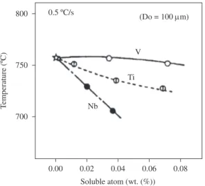
Niobium and titanium have been found to significantly affect the austenite decomposition kinetics3-5. An example
of the effect of niobium and titanium in solution on the transformation start temperature is shown in Figure 1, which indicates that both niobium and titanium have a strong effect on delaying the start of the proeutectoid ferrite transformation, and that niobium is more effective for this delay than titanium. In addition, niobium and titanium have different affinities for carbon and nitrogen in austenite as shown in Figure 2, so that precipitates of carbides, nitrides and carbonitrides are formed for both niobium and titanium.
Coarse grain boundary precipitates have been found to be potent nucleation sites for ferrite formation due to the large mismatch with austenite which provides a high energy interface suitable for nucleation4. In addition, the
formation of these coarse precipitates locally reduces the niobium and carbon contents in solution resulting in the effect of solute drag to be decreased and further promoting ferrite nucleation.
Cooling rate is one of the key parameters, which can be adapted on a welding due to its strong effect on the kinetics of austenite decomposition and resulting microstructure6.
A wide variety of transformation products i.e. polygonal ferrite, acicular ferrite, bainite and/or martensite, can be obtained in HSLA steels by changing the cooling conditions during the continuous cooling phase transformation.
Austenite decomposition is a thermally activated process where the formation of the new product phase requires time to initiate nucleation and to continue into the growth stage. As a result, by increasing the cooling rate the available time at any given temperature to start the nucleation and growth processes is diminished, and thus, shifts the transformation start to lower temperatures6-9. Increasing the
and growing ferrite which leads to the activation of more potential nucleation sites10. At very high cooling rates, the
transformation rate decreases due to a reduction in the diffusivity of carbon.
In addition to producing a finer ferrite grain size, an increase in the cooling rate can also form low temperature secondary products such as bainite and martensite due to the repression of the transformation start temperature. By controlling the final microstructure through cooling the desired–final mechanical properties of the steel can be achieved. In this way, controlled cooling on the weld heat affected zone (HAZ) is an important thermal treatment which can effectively control the final microstructure and mechanical properties of the steel.
The initial austenite microstructure plays an important role in the transformation behavior for weld HAZ cooling. The two microstructural features of austenite which are important for the transformation process include the austenite grain size and the degree of precipitation.
The heterogeneous nucleation of ferrite occurs prevalently on austenite grain boundaries. Therefore, a decrease of the austenite grain size leads to an increase in the grain boundary area per unit volume and thus a greater surface area for potential nucleation sites. As a result of increasing the number of potential nucleation sites, transformation starts at higher temperatures and produces higher temperature transformation products such as polygonal ferrite6,11. A finer ferrite grain size is produced
since the number of ferrite formed increases due to more available potential nucleation sites where impingement of the growing ferrite grains will occur earlier due to the decrease of the austenite grain size.
It is observed that with a decrease in the austenite grain size, the transformation rate increases due to the increase in the ratio of nucleation rate to growth rate12-13. In addition,
formation of polygonal ferrite is depressed with an increase in the austenite grain size and formation of non-polygonal microstructures is promoted6.
Several works have addressed utilizing of computer-aided prediction of engineering properties including those done by the authors14-19. Adaptive Network-based
Fuzzy Inference Systems (ANFIS) is the famous hybrid neuro-fuzzy network for modeling the complex systems20.
ANFIS incorporates the human-like reasoning style of fuzzy systems through the use of fuzzy sets and a linguistic model consisting of a set of IF–THEN fuzzy rules. The main strength of ANFIS models is that they are universal approximators20 with the ability to solicit interpretable IF–
THEN rules. Nowadays, the artificial intelligence-based techniques like ANFIS21 have been successfully applied in
the engineering applications. However, there is a lack of investigations on metallurgical aspects of materials.
In the present study, the effects of chemical compositions, austenitizing temperature, austenitic grain size and cooling rate on Vickers microhardness of low-carbon microalloyed steels has been modeled by ANFIS. Totally 114 Vickers microhardness data were collected from the literature, trained, tested and validated by ANFIS. The obtained results were compared by experimental ones to evaluate the software power for predicting the effects of mentioned parameters on microhardness of the studied steels.
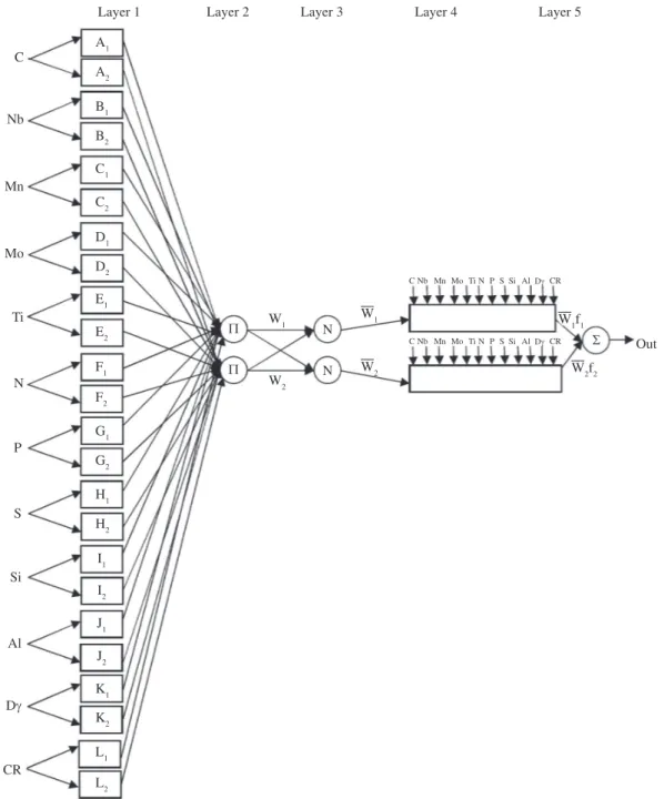
2. Architecture of ANFIS
The architecture of an ANFIS model with two input variables is shown in Figure 3. Suppose that the rule base
Figure 2. Solubility products of niobium, aluminium, vanadium and titanium nitrides and carbides4.
0.00 0.02 0.04 0.06 0.08
Soluble atom (wt. (%)) 700
800 0.5 ºC/s (Do = 100 µm)
V
Ti
Nb 750
T
emperature (ºC)
Figure 1. The effect of niobium and titanium in solution on the transformation start temperature (Ae3)
of ANFIS contains two fuzzy IF–THEN rules of Takagi and Sugeno’s type as follows:
Rule 1: IF × is A1 and y is B1, THEN f1 = p1x + q1y + r1. Rule 2: IF × is A2 and y is B2, THEN f2 = p2x + q2y + r2. In Figure 3 fuzzy reasoning is illustrated and also the corresponding equivalent ANFIS architecture is shown in Figure 4. The functions of each layer are explained as follows23-27:
Layer 1 – Every node i in this layer is a square node with a node function:
( )
1
i
i A
O = µ x (1)
(fuzzy sets: small, large, …) associated with this node function.
Layer 2 – Every node in this layer is a circle node labeled P, which multiplies the incoming signals and sends the product out. For instance,
( )
( )
1, 2i i
i A B
W= µ y × µ y i= (2)
Each node output represents the firing weight of a rule. Layer 3 – Every node in this layer is a circle node labeled N. The ith node calculates the ratio of the ith rule’s firing weight to the sum of all rule’s firing weights:
Wi = Wi / (W1 / W2), i = 1,2 (3)
Layer 4 – Every node in this layer is a square node with a node function:
(
)
4
i i i i i
O =W P X+q y r+ (4)
where Wi is the output of layer 3, and {pi, qi, ri} is the parameter set.
Layer 5 – The signal node in this layer is a circle node labeled R that computes the overall output as the summation of all incoming signals, that is,
5 /
i i i i i i i i i
O = ∑ W f= ∑W f ∑W (5)
The basic learning rule of ANFIS is the back-propagation gradient descent, which calculates error signals recursively from the output layer backward to the input nodes. This learning rule is exactly the same as the
back-propagation learning rule used in the common feed-forward neural networks28,29. Newly, ANFIS adopted a
rapid learning method named as hybrid-learning method that utilizes the gradient descent and the least-squares method to find a feasible set of antecedent and consequent parameters28,29. Therefore, in this paper, the later method is
used for constructing the proposed models.
3. Training and Verifying
3.1.
Data collection
In the present investigation, the ANFIS has been trained, tested and validated for prediction microhardness of low-carbon microalloyed steels. For this purpose, the experimental data of five low-carbon microalloyed steels with different chemical compositions have been used30-34.
The chemical compositions of these steels are summarized in Table 1. The input variables of the ANFIS modeling are the weight percent of alloying elements, the initial austenite grain size and the cooling rate. These parameters along with their ranges have been summarized in Table 2.
3.2.
ANFIS model structure and parameters
The structure of proposed ANFIS networks consisted of twelve input variables including the carbon concentration (cC), the niobium concentration(cNb), the manganese concentration(cMn), the molybdenum concentration (cMo), the titanium concentration (cTi), the nitrogen concentration (cN), the phosphorous concentration (cP), the sulfur concentration (cS), the silicon concentration nt (cSi), the aluminum concentration (cAl), the initial austenite grain size (Dγ) and the cooling rate (CR). The value for output layer was the Vickers microhardness (HV).
Figure 3. The reasoning sheme of ANFIS22.
The input space is decomposed by three fuzzy labels. In this paper, for comparison purposes, two types of membership functions (MFs) including the triangular (ANFIS-I) and Gaussian (ANFIS-II) were utilized to construct the suggested models. The ANFIS models were trained, from 114 collected data, by 80 data (70%) were randomly chosen for training set, 17 (15%) data for testing set and the other 17 (15%) data for validation set. Moreover, up to 1,000 epochs were specified for training process to assure the gaining of the minimum error tolerance.
One of the most difficult tasks in ANFIS studies is to find this optimal network architecture, which is based on the determination of numbers of optimal results. The assignment of initial weights and other related parameters may also influence the performance of the ANFIS to a great extent. However, there is no well defined rule or procedure to have an optimal network architecture and parameter settings where the trial and error method still remains valid. This process is very time consuming.
In this study, the Matlab ANFIS toolbox is used for ANFIS applications. To overcome optimization difficulty, a program has been developed in Matlab, which handles the trial-and-error process automatically35-38. The program
tries various functions and when the highest RMSE (root mean squared error) of the testing set, as the training of the testing set, is achieved, it was reported35-38.
The IF–THEN rules in this study were achieved as follows. Suppose that the rule base of ANFIS contains two fuzzy IF–THEN rules of Takagi and Sugeno’s type:
Rule 1: IF cC is A1, cNb is B1, cMn is C1, cMo is D1, cTi is E1, cN is F1, cP is G1, cS is H1, cSi is I1, cAl is J1, Dγ is K1 and CR is L1
T H E N f1 = n1c C + o1c N b + p1c M n + q1cMo + r1cTi + s1cN + t1cP+ u1cS + v1cSi + w1cAl + x1 Dγ + y1CR + zb1.
Rule 2: IF cC is A2, cNb is B2, cMn is C2, cMo is D2, cTi is E2, cN is F2, cP is G2, cS is H2, cSi is I2, cAl is J2, Dγ is K2 and CR is L2
T H E N f2 = n2c C + o2c N b + p2c M n + q2cMo + r2cTi + s2cN + t2cP+ u2cS + v2cSi + w2cAl + x2 Dγ + y2CR + zb2.
The corresponding equivalent ANFIS architecture is shown in Figure 5. The functions of each layer are described as follows:
Layer 1 – Every node i in this layer is a square node with a node function:
( )
1
1, 2
i
i A
O = µ cC i= (6)
( )
1 1, 2
i
i B
O = µ cNb i= (7)
(
)
1 1, 2
i
i C
O = µ cMn i= (8)
(
)
1 1, 2
i
i D
O = µ cMo i= (9)
( )
1
1, 2
i
i E
O = µ cTi i= (10)
( )
1 1, 2
i
i F
O = µ cN i= (11)
( )
1
1, 2
i
i G
O = µ cP i= (12)
( )
1
1, 2
i
i H
O = µ cS i= (13)
( )
1 1, 2
i
i I
O = µ cSi i= (14)
Table 1. Chemical composition of the microalloyed steels.
Ref. Steel Chemical composition (wt. (%))
C Mn Nb Mo Ti N P S Si Al
26 X80 0.060 1.650 0.034 0.240 0.012 0.005 0.000 0.000 0.000 0.000
27 HSLA65 0.062 1.240 0.063 0.008 0.002 0.007 0.007 0.004 0.051 0.040
27 HSLA 90 0.050 1.650 0.071 0.196 0.021 0.000 0.010 0.004 0.025 0.027
28 Nb steel 0.060 1.200 0.062 0.000 0.000 0.008 0.000 0.007 0.290 0.035
29 Nb-Mo steel 0.050 1.880 0.049 0.490 0.000 0.004 0.005 0.007 0.040 0.050
30 DP600 0.060 1.860 0.000 0.155 0.011 0.007 0.015 0.004 0.077 0.043
Table 2. The parameters and their range used in the neural network.
Parameter Range
Input
C (wt. (%)) 0.050-0.062
Mn (wt. (%)) 1.200-1.880
Nb (wt. (%)) 0.000-0.071
Mo (wt. (%)) 0.008-0.490
Ti (wt. (%)) 0.000-0.021
N (wt. (%)) 0.000-0.007
P (wt. (%)) 0.000-0.015
S (wt. (%)) 0.000-0.007
Si (wt. (%)) 0.000-0.077
Al (wt. (%)) 0.000-0.050
Dγ (µm) 5-130
CR (°C) 0.3-153
Output
( )
1 1, 2
i
i J
O = µ cAl i= (15)
( )
1 1, 2
i
i K
O = µ Dγ i= (16)
( )
1 1, 2
i
i L
O = µ CR i= (17)
where cC, cNb, cMn, cMo, cTi, cN, cP, cS, cSi, cAl, Dγ and CR are inputs to node i, and Ai, Bi, Ci, Di, Ei, Fi,Gi, Hi. Ii, Ji, Ki and Li are the linguistic label (fuzzy sets: small, large, …) associated with this node function.
Layer 2 – Every node in this layer is a circle node labeled Πwhich multiplies the incoming signals and sends the product out. For instance,
( )
( )
( ) ( )( ) ( ) ( ) ( ) ( )
( ) (D ) ( ), 1, 2
i i i i
i i i i i
i i i
i A B C D
E F G H I
J K L
W cC cNb cMn cMo
cTi cN cP cS cSi
cAl CR i
= µ × µ × µ × µ ×
× µ × µ × µ × µ × µ ×
× µ × µ γ × µ =
(18)
Each node output represents the firing weight of a rule. Layer 3 – Every node in this layer is a circle node labeled N. The ith node calculates the ratio of the ith rule’s firing weight to the sum of all rule’s firing weights:
(
1 2)
/ / , 1, 2
i i
W =W W W i= (19)
Layer 4 – Every node in this layer is a square node with a node function:
4 i i i i i i
i i
i i i i i i i
n cC o cNb p cMn q cMo r cTi s cN
O w
t cP u cS v cSi w cAl x D y CR zb
+ + + + + +
=
+ + + + + γ + +
(20)
where Wi is the output of layer 3, and {ni, oi, pi, qi, ri, si, ti, ui, vi, wi, xi, yi, zi} is the parameter set.
Layer 5 – The signal node in this layer is a circle node labeled R that computes the overall output as the summation of all incoming signals, i.e.,
5
/ i i i i i i i i i
O = ∑ w f= ∑ w f ∑w (21)
4. Results and Discussion
4.1.
The effects of austenitizing temperature and
cooling rate
The austenite decomposition is heavily influenced by the initial austenite grain size and cooling rate. For a given cooling rate, an increase in austenite grain size results in lower transformation start temperatures resulting in a decrease in polygonal ferrite fraction. Further, for a given austenite grain size, accelerated cooling lowers the transformation start temperature with an associated decrease
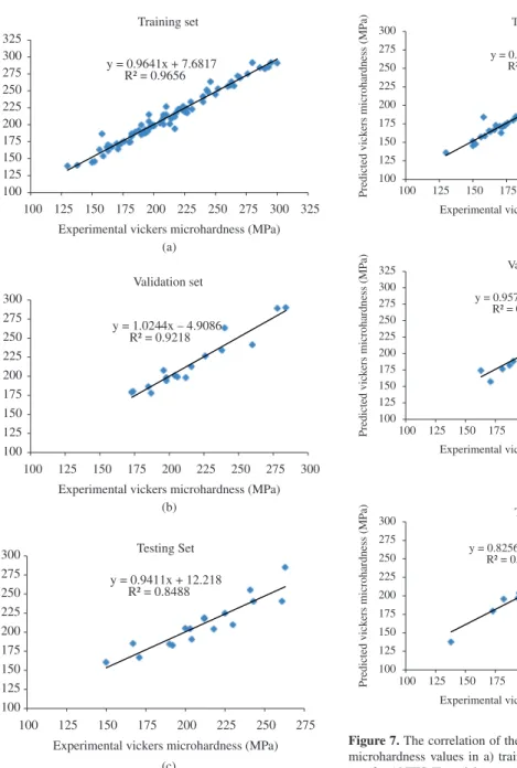
Figure 6. The correlation of the measured and predicted Vickers microhardness values in a) training, b) validation and c) testing sets for ANFIS-I model.
in the polygonal ferrite fraction in addition to refining the resulting ferrite grains. Accelerated cooling in combination with smaller austenite grain sizes further refines the ferrite grains. The effect of processing variables indicates that the hardness increases with austenite grain size and cooling rate as a result of the decrease in transformation start temperature where low temperature transformation products are formed, i.e. bainite and martensite, which are harder phases.
Predicting the microstructural evolution under continuous cooling conditions as found on the welding is a challenging task since in addition to cooling conditions, the austenite decomposition is affected by chemistry, austenite grain size and retained strain. There is a clear shift of the transformation kinetics to lower transformation temperatures with an increase in the initial austenite grain size. A larger initial austenite grain size provides less
boundary surface area per unit volume, thus reducing the number of available nucleation sites for ferrite and as a result transformation occurs at lower temperatures. In addition, the carbon diffusion distance is greater for a larger initial austenite grain size requiring additional time for diffusion, thereby lowering the transformation temperature. The shift to lower transformation start temperatures for an increase in the initial austenite grain size, is associated with the delay of transformation start for larger austenite grains since, comparatively they provide fewer nucleation sites. Similar trends were observed for transformation finish temperatures. The increase in cooling rate and/or initial austenite grain size gave rise to a significant increase in the hardness of the steel. For example, for HSLA 90[27] an increase in the cooling
rate from 1 to 179 °C/s increased the hardness by 90 HV for an austenite grain size of 53 µm and for an increase in the
Table 3. Testing and validation data sets for comparison of experimental results with testing and validation results predicted from ANFIS-I model.
The set name
Chemical composition (wt. (%))
Austenite Grain size
Cooling rate
Vickers microhardness
C Nb Mn Mo Ti N P S Si Al dγ (µm) CR (°C) Exp. Pred.
Validation 0.06 1.65 0.034 0.24 0.012 0.005 0 0 0 0 5 3 260 241.4
0.06 1.65 0.034 0.24 0.012 0.005 0 0 0 0 5 60 212 198.4
0.06 1.65 0.034 0.24 0.012 0.005 0 0 0 0 80 60 226 226.8
0.06 1.65 0.034 0.24 0.012 0.005 0 0 0 0 15 60 198 198.4
0.06 1.65 0.034 0.24 0.012 0.005 0 0 0 0 80 30 240 263.5
0.062 1.24 0.063 0.008 0.002 0.007 0.007 0.004 0.051 0.04 19 125 174 180.3 0.062 1.24 0.063 0.008 0.002 0.007 0.007 0.004 0.051 0.04 49 10 187 178.1 0.062 1.24 0.063 0.008 0.002 0.007 0.007 0.004 0.051 0.04 49 55 204 201.1 0.062 1.24 0.063 0.008 0.002 0.007 0.007 0.004 0.051 0.04 130 5 198 194.2 0.062 1.24 0.063 0.008 0.002 0.007 0.007 0.004 0.051 0.04 130 15 206 199.2 0.05 1.65 0.071 0.196 0.021 0 0.01 0.004 0.025 0.027 32 63 238 234.2 0.05 1.65 0.071 0.196 0.021 0 0.01 0.004 0.025 0.027 53 1 196 207.8 0.05 1.65 0.071 0.196 0.021 0 0.01 0.004 0.025 0.027 53 127 284 290.1 0.06 1.86 0 0.155 0.011 0.007 0.015 0.004 0.077 0.043 16 23 173 179.2 0.06 1.86 0 0.155 0.011 0.007 0.015 0.004 0.077 0.043 16 67 216 212.9
0.05 1.88 0.049 0.49 0 0.004 0.005 0.007 0.04 0.05 20 1 185 186.5
0.05 1.88 0.049 0.49 0 0.004 0.005 0.007 0.04 0.05 62 100 278 289.3
Testing 0.06 1.65 0.034 0.24 0.012 0.005 0 0 0 0 42 60 225 225
0.06 1.65 0.034 0.24 0.012 0.005 0 0 0 0 42 100 203 204.7
0.06 1.65 0.034 0.24 0.012 0.005 0 0 0 0 80 100 204 190.7
0.06 1.65 0.034 0.24 0.012 0.005 0 0 0 0 24 30 243 240.5
0.06 1.65 0.034 0.24 0.012 0.005 0 0 0 0 80 10 263 285.2
0.062 1.24 0.063 0.008 0.002 0.007 0.007 0.004 0.051 0.04 49 18 192 182.9 0.062 1.24 0.063 0.008 0.002 0.007 0.007 0.004 0.051 0.04 49 110 212 217.9 0.062 1.24 0.063 0.008 0.002 0.007 0.007 0.004 0.051 0.04 49 192 218 204.3 0.05 1.65 0.071 0.196 0.021 0 0.01 0.004 0.025 0.027 14 172 230 209.8 0.05 1.65 0.071 0.196 0.021 0 0.01 0.004 0.025 0.027 32 1 190 184.6 0.05 1.65 0.071 0.196 0.021 0 0.01 0.004 0.025 0.027 32 172 261 240.7 0.05 1.65 0.071 0.196 0.021 0 0.01 0.004 0.025 0.027 53 12 212 218.9 0.06 1.86 0 0.155 0.011 0.007 0.015 0.004 0.077 0.043 16 1 150 160.6 0.06 1.86 0 0.155 0.011 0.007 0.015 0.004 0.077 0.043 24 5 171 166.8
0.05 1.88 0.049 0.49 0 0.004 0.005 0.007 0.04 0.05 8 1 167 185.3
0.05 1.88 0.049 0.49 0 0.004 0.005 0.007 0.04 0.05 20 100 241 255.6
austenite grain size from 14 to 53 µm, the hardness increased by 58 HV for a cooling rate of 127 °C/s.
The observed increase in hardness obtained by increasing the cooling rate is related to a decrease in the transformation temperatures for which non-polygonal products, i.e. harder phases are formed. In addition, decreasing the austenite grain size also results in an increase in hardness; this is due to the refinement of ferrite grains with a decrease in the austenite grain size.
4.2.
ANFIS modeling
In this study, the error arose during the training, Validation and testing in ANFIS-I and ANFIS-II models can be expressed as absolute fraction of variance (R2) which is
calculated by Equation 2:
(
)
( )
2 2
2
1 – i i i
i i
t o
o R
=
−
∑
∑ (22)
where t is the target value and o is the output value. All of the results obtained from experimental studies and predicted by using the training, testing and validation results of ANFIS-I and ANFIS-II models are given in Figures 6a-c and 7a-c, respectively. The linear least square fit line, its equation and R2 values were shown in these figures for the
training, testing and validation data. Also, inputs values and experimental results with testing and validation results obtained from ANFIS-I and ANFIS-II models were given in Tables 3 and 4, respectively. As it is visible in Figures 6 and 7, the values obtained from the training, testing and validation sets in ANFIS-I and ANFIS-II models are very
Table 4. Testing and validation data sets for comparison of experimental results with testing and validation results predicted from ANFIS-II model.
The set name
Chemical composition (wt. (%))
Austenite Grain size
Cooling rate
Vickers Microhardness
C Nb Mn Mo Ti N P S Si Al dγ (µm) CR (°C) Exp. Pred.
Validation 0.06 1.65 0.034 0.24 0.012 0.005 0 0 0 0 42 3 300 293.6
0.06 1.65 0.034 0.24 0.012 0.005 0 0 0 0 42 10 290 284.3
0.06 1.65 0.034 0.24 0.012 0.005 0 0 0 0 42 60 225 226.4
0.06 1.65 0.034 0.24 0.012 0.005 0 0 0 0 80 60 210 227.4
0.062 1.24 0.063 0.008 0.002 0.007 0.007 0.004 0.051 0.04 49 5 181 176.7 0.062 1.24 0.063 0.008 0.002 0.007 0.007 0.004 0.051 0.04 49 10 187 182.3 0.062 1.24 0.063 0.008 0.002 0.007 0.007 0.004 0.051 0.04 49 110 212 201.8 0.062 1.24 0.063 0.008 0.002 0.007 0.007 0.004 0.051 0.04 49 192 218 215.1 0.062 1.24 0.063 0.008 0.002 0.007 0.007 0.004 0.051 0.04 130 198 227 235.1 0.05 1.65 0.071 0.196 0.021 0 0.01 0.004 0.025 0.027 14 1 163 174.3 0.05 1.65 0.071 0.196 0.021 0 0.01 0.004 0.025 0.027 14 172 230 234.2 0.05 1.65 0.071 0.196 0.021 0 0.01 0.004 0.025 0.027 32 1 190 188.3 0.05 1.65 0.071 0.196 0.021 0 0.01 0.004 0.025 0.027 53 12 212 214.2 0.05 1.65 0.071 0.196 0.021 0 0.01 0.004 0.025 0.027 53 127 284 276.7 0.06 1.86 0 0.155 0.011 0.007 0.015 0.004 0.077 0.043 16 5 171 157.5 0.06 1.86 0 0.155 0.011 0.007 0.015 0.004 0.077 0.043 24 48 205 205.1 0.06 1.86 0 0.155 0.011 0.007 0.015 0.004 0.077 0.043 24 157 260 255.9
Testing 0.06 1.65 0.034 0.24 0.012 0.005 0 0 0 0 42 100 203 200.6
0.06 1.65 0.034 0.24 0.012 0.005 0 0 0 0 80 3 295 275.7
0.06 1.65 0.034 0.24 0.012 0.005 0 0 0 0 80 10 293 268.8
0.06 1.65 0.034 0.24 0.012 0.005 0 0 0 0 5 3 240 246.4
0.06 1.65 0.034 0.24 0.012 0.005 0 0 0 0 5 30 208 218
0.06 1.65 0.034 0.24 0.012 0.005 0 0 0 0 80 100 195 203.8
0.062 1.24 0.063 0.008 0.002 0.007 0.007 0.004 0.051 0.04 19 2.5 138 137.8 0.05 1.65 0.071 0.196 0.021 0 0.01 0.004 0.025 0.027 14 20 182 195.7 0.05 1.65 0.071 0.196 0.021 0 0.01 0.004 0.025 0.027 32 6.7 194 197.2 0.05 1.65 0.071 0.196 0.021 0 0.01 0.004 0.025 0.027 32 17 199 211 0.05 1.65 0.071 0.196 0.021 0 0.01 0.004 0.025 0.027 32 120 243 251.7 0.05 1.65 0.071 0.196 0.021 0 0.01 0.004 0.025 0.027 53 5 208 202.9 0.06 1.86 0 0.155 0.011 0.007 0.015 0.004 0.077 0.043 16 23 173 179.6 0.06 1.86 0 0.155 0.011 0.007 0.015 0.004 0.077 0.043 32 155 270 260.2
0.05 1.88 0.049 0.49 0 0.004 0.005 0.007 0.04 0.05 8 15 200 194.7
0.05 1.88 0.049 0.49 0 0.004 0.005 0.007 0.04 0.05 8 40 225 220.4
close to the experimental results. The results of testing and validation phases in Figures 6 and 7 show that the ANFIS-I and ANFIS-II models are capable of generalizing between input and output variables with reasonably good predictions.
The performance of the ANFIS-I and ANFIS-II models is shown in Figures 6 and 7. The best value of R2 is 96.56%
for training set in the ANFIS-I model. The minimum values of R2 are 97.23% for training set in the ANFIS-II model. All
of R2 values show that the proposed ANFIS-I and ANFIS-II
models are suitable and can predict Vickers microhardness of microalloyed steels values very close to the experimental values.
5. Conclusion
1. The effect of processing variables shows that the hardness of steels increases with the increase of austenite grain size and cooling rate attributed to the
increase in non-polygonal structures which show a higher hardness. This effect can be rationalized with transformation temperature, e.g. a decreasing transformation start temperature leads to higher hardness values; and
2. The ANFIS approach appears to be a very powerful tool in materials engineering. The results presented show that the prediction of the microhardness properties of the considered steel is in a good agreement with the experimental data. The ANFIS was trained, Tested and validated on the data obtained from the literature. The accuracy of values evaluated by the ANFIS model is much higher than that obtained from calculations using the classical, experimental models. This means that the well-trained network under laboratory conditions is able to predict the correct values of the output parameters of the industrial process.
References
1. DeArdo AJ. Modern thermomechanical processing of microalloyed steel: A physical metallurgy perspective.
In: Proceedings of Microalloying ‘95 Conference; 1995;
Pittsburgh. ISS; 1995. p. 15-33.
2. Ouchi C. Development of Steel Plates by Intensive Use of TMCP and. Direct Quenching Processes. ISIJ
International. 2001;14:542-553. http://dx.doi.org/10.2355/
isijinternational.41.542
3. Kwon O and DeArdo AJ. Interactions between recrystallization and precipitation in hot-deformed microalloyed steels. Acta
Metallurgica et Materialia. 1991; 39(4):529-38. http://dx.doi.
org/10.1016/0956-7151(91)90121-G
4. Volb-ath LGE, Hackl R, Schmitt-Thomas KG and Daub D. Influence of TM-Rolling Parameters on Properties of Microalloyed Cold Rolled Steels. In: Microalloying ‘88; 1988; Metals Park. ASM 1988. p. 353-358.
5. Honeycombe R and Bhadeshia H. Steels: Microstructure and Properties. London: Edward Arnold; 1995.
6. Tamura I, Ouchi C, Tanaka T and Sekine H. Thermomechanical
Processing of High Strength Low Alloy Steels. London:
Butterworths; 1998. p. 21.
7. Okaguchi S, Hasimoto T and Ohtani H. Effect of Nb, V and Ti on Transformation Behavior of HSLA. Steel in Accelerated Cooling. In: THERMEC’88; 1988. IS1J, 1988. vol. 1, p. 330. 8. Oberhauser F, Listhuber F and Wallener F. Microalloying Steels
for Light, Cold-Formed Sections. In: Mircoalloying’75; 1975; New York. Union Carbide Corporation; 1977. p. 665. 9. Collins L and Liu W. Phase Transformation During the
Thermal/Mechanical Processing of Steel. The Metallurgical
Society of CIM; 1995. p. 419.
10. Pandi R. Modelling of Austenite to Ferrite Transformation Behaviour in Low Carbon Steels During Run-out
Table Cooling. [Dissertation]. Vancouver: The University of
British Columbia; 1998.
11. Militzer M, Pandi R and Hawbolt B. Ferrite nucleation and growth during continuous cooling. Metallurgical and
Materials Transactions A. 1996; 27(6):1547-1556. http://
dx.doi.org/10.1007/BF02649814
12. M i l i t z e r M , H a w b o l t B a n d M e a d o w c r o f t R . Microstructural model for hot strip rolling of high-strength low-alloy steels. Metallurgical and Materials
Transactions. 2000; 31(4):1247-1259. http://dx.doi.
org/10.1007/s11661-000-0120-4
13. Militzer M, Hawbolt B and Meadowcroft R. Phase Transformation During the Thermal/Mechanical Processing
of Steel. The Metallurgical Society of CIM; 1995. p. 445.
14. Porter DA and Easterling KE. Phase Transformations in Metals
and Alloys. 2nd ed. London: Chapman and Hall; 1992.
15. Nakata N and Militzer M. Microstructure Evolution of a State-of-the-Art Ti-Nb HSLA Steel. In: Mechanical Working and
Steel Processing Conference Proceedings; 2000; Warrendale.
ISS; 2000. vol. 38, p. 813.
16. Hawbolt B, Chau B and Brimacombe K. Mathematical
Modelling of Hot Rolling of Steel. Canada: The Metallurgical
Society of CIM; 1990. p. 424.
17. Pandi R, Militzer M, Hawbolt B and Meadowcroft R. Effect of Cooling and Deformation on the Austenite Decomposition Kinetics. In: Proceedings of 37th Mechanical Working and Steel
Processing Conference; 1995; Warrendale. ISS; 1995. p. 635.
18. Nazari A and Milani AA. Modeling ductile to brittle transition temperature of functionally graded steels by artificial neural networks. Computational Materials
Science. 2011; 50:2028-2037. http://dx.doi.org/10.1016/j.
commatsci.2011.02.003
19. Nazari A and Milani AA. Modeling ductile to brittle transition temperature of functionally graded steels by fuzzy logic.
Journal of Materials Science. 2011; 46(18):6007-6017. http://
dx.doi.org/10.1007/s10853-011-5563-z
20. Nazari A and Riahi S. Computer-aided prediction of physical and mechanical properties of high strength cementitious composite containing Cr2O3 nanoparticles. Nano. 2010; 5(5):301-318. http://dx.doi.org/10.1142/S1793292010002219
21. Nazari A and Riahi S. Prediction split tensile strength and water permeability of high strength concrete containing TiO2 nanoparticles by artificial neural network and genetic programming. Composites Part B: Engineering. 2011; 42:473-488. http://dx.doi.org/10.1016/j. compositesb.2010.12.004
22. Nazari A and Riahi S. Computer-aided design of the effects of Fe2O3 nanoparticles on split tensile strength and water
permeability of high strength concrete. Materials and
Design. 2011; 32:3966-3979. http://dx.doi.org/10.1016/j.
matdes.2011.01.064
23. N a z a r i A a n d D i d e h v a r N . M o d e l i n g i m p a c t resistance of aluminum-epoxy laminated composites. ANFIS. 2011; 42:1912-1919.
and Cybernetics. 1993; 23(3):665-85. http://dx.doi. org/10.1109/21.256541
25. Saridemir M. Predicting the compressive strength of mortars containing metakaolin by artificial neural networks and fuzzy logic. Advances in Engineering Software. 2009; 40(9):920-7. http://dx.doi.org/10.1016/j.advengsoft.2008.12.008
26. Ramezanianpour AA, Sobhani M and Sobhani J. Application of network based neuro-fuzzy system for prediction of the strength of high strength concrete. Amirkabir Journal of Science and
Technology. 2004; 5(59-C):78-93.
27. Ramezanianpour AA, Sobhani J and Sobhani M. Application of an adaptive neurofuzzy system in the prediction of HPC compressive strength. In: Proceedings of the 4th international
conference on engineering computational technology; 2004;
Lisbon. Lisbon: Civil-Comp Press; 2004. p. 138.
28. Topcu IB and Sarıdemir M. Prediction of mechanical properties of recycled aggregate concretes containing silica fume using artificial neural networks and fuzzy logic.
Computational Materials Science. 2008; 42(1):74-82. http://
dx.doi.org/10.1016/j.commatsci.2007.06.011
29. Jang JSR and Sun CT. Nuro-fuzzy modeling and control. Proceedings of IEEE. 1995; 83(3). http://dx.doi. org/10.1109/5.364486
30. Tafteh R. Austenite decomposition in an X80 linepipe steel. [Thesis]. The University of British Columbia; 2011. 31. Lottey KK. Austenite decomposition of a HSLA-Nb, Ti steel
and an A1-TRIP steel during continuous cooling. [Thesis]. The
University of British Columbia; 2002.
32. Olasolo M, Uranga P, Rodriguez-Ibabe JM and López B. Effect of austenite microstructure and cooling rate on transformation characteristics in a low carbon Nb–V microalloyed steel.
Materials Science and Engineering A. 2011; 528:2559-2569.
http://dx.doi.org/10.1016/j.msea.2010.11.078
33. Petkov P. Austenite decomposition of low carbon high strength
steels during continuous cooling. [Thesis]. The University of
British Columbia; 2004.
34. Sarkar S. Microstructural evolution model for hot strip rolling
of a Nb-Mo complex-phase steel. [Thesis]. The University of
British Columbia; 2008.
35. Guzelbey IH, Cevik A and Erklig A. Prediction of web crippling strength of cold-formed steel sheetings using neural Networks.
Journal of Constructional Steel Research. 2006; 62:962-973.
http://dx.doi.org/10.1016/j.jcsr.2006.01.008
36. Guzelbey IH, Cevik A and Gögüs MT. Prediction of rotation capacity of wide flange beams using neural Networks. Journal
of Constructional Steel Research. 2006; 62:950-961. http://
dx.doi.org/10.1016/j.jcsr.2006.01.003
37. Cevik A and Guzelbey IH. Neural network modeling of strength enhancement for CFRP confined concrete cylinders.
Building and Environment. 2008; 43:751-763. http://dx.doi.
org/10.1016/j.buildenv.2007.01.036