J. Braz. Comp. Soc. vol.13 número2

(1)

Filter to Localize Multi

Autonomous Underwater Vehicles

∗

Silvia Botelho

1

, Renato Neves

2

, Lorenzo Taddei

3

& Vinícius Oliveira

1

1_{Computer Engineering}

Federal University of Rio Grande - FURG Av. Itália km 8, Campus Carreiros

Phone: +55 (53) 32336623

Zip 96201-090 - Rio Grande - RS - BRAZIL {silviacb | dmtvmo }@furg.br

2_{Institute of Computing}

State University of Campinas

P.O.Box 6176, Zip 13084-971 - Campinas - SP - BRAZIL renato.neves@students.ic.unicamp.br

3_{Electric Engineering}

Federal University of Rio Grande do Sul- UFRGS Av. Osvaldo Aranha, 103 - Sala 208

Phone: +55 (51) 3316.3515

Zip 90035-190 - Porto Alegre - RS - BRAZIL lorenzo@delet.ufrgs.br

Abstract

The present paper describes a system for the construc-tion of visual maps (“mosaics”) and moconstruc-tion estimaconstruc-tion for a set of AUVs (Autonomous Underwater Vehicles). Robots are equipped with down-looking camera which is used to estimate their motion with respect to the seafloor and built an online mosaic. As the mosaic increases in size, a systematic bias is introduced in its alignment, re-sulting in an erroneous output. The theoretical concepts associated with the use of an Augmented State Kalman Filter (ASKF) were applied to optimally estimate both vi-sual map and the fleet position.

Keywords: Multi-Robots, Autonomous Underwater Vehicles, Mosaics, Robotic Localization

∗_{This work was sponsored by Conselho Nacional de Pesquisa (CNPq)}

1. I

NTRODUCTION

(2)

highly used by the marine community.

For visual-based underwater exploration, UUVs are equipped with down-looking cameras that produce im-ages from the bottom of the sea, providing a visual map during the vehicle navigation. Every frame captured by the vehicle is used to compose the map. Consecutive frames are aligned and then a final map is generated, which is called mosaic [16]. Mosaics can also be used as reference maps in the navigation/localization vehicle process [5]. This visual map can be used either in the surface for seabed exploration or for a visual-based AUV localization/navigation. Thus, the vehicle is able to navi-gate using its own online map. Given the vehicle altitude above the ocean floor (e.g. from an altimeter) and cam-era field of view, the actual area covered by the map (and individual frames) is known, the navigation in real world coordinates is possible.

A cumulative error, however, is introduced in the alignment of the consecutive frames within the mosaic. GPSs placed on the surface and Acoustic Transponder Network (ATN) distributed in the exploration area are sensorial approaches, which can be used to correct this kind of drift [15, 11], but both have similar disadvantages: a high cost of operation, and a restrict range of applica-tion (small depth, ATNs areas, etc).

Occasionally, the robot path may be crossed-over, [5] proposes a smooth adjustment of the mosaic cumulative error detected by the crossover points in the map construc-tion. [7] uses Augmented State Kalman Filter (ASKF) to estimate the correct position of both the vehicle and every frame of the mosaic, based on crossover and displacement measurements [4]. The ASKF strategies for the mosaic update and vehicle localization take into account simpli-fied dynamic model of the AUV, as well as the detected crossover regions, which is very important to the accuracy of the system.

1.1. MULTI-AUVSFORVISUALMAPPING

Two issues are considered in this paper: i. High costs and the complexity associated with more sophisticated and long missions unable the massive use of AUVs. On the other hand, simple vehicles are incapable to accom-plish trivial tasks due to their low autonomy, poor number of sensors and other limitations. ii. The possibility of using its own explored image as information to localize the vehicle is an attractive and low cost operation. ASKF seems to be a good choice, specifically when the naviga-tion provides a set of crossover regions.

In this context, we argue that a fleet of simple robots can be more efficient than a sophisticated AUV to seabed exploration tasks. A heterogeneous fleet can be composed by robots equipped with different sensors and no complex power supply systems. These simple vehicles would ex-plore a region in a fraction of time needed by a single

AUV. Mosaics would be more efficiently constructed and their visual information would be used to help the local-ization and navigation of the fleet.

We have a set of real situations where this approach could be applied. For instance, in northeast of the Brazil-ian Coast we have a protected reef of chorales area, called “Parrachos de Maracajau”. This is a wide area, where a continuous visual inspection is important. Due to the need of a continuous mapping the sea-divers-based inspection is very expensive. In this case, the use of a robotic ve-hicle may be a good choice. Besides, the veve-hicle can use the visual information as sensorial input for its local-ization/navigation system, avoiding boring human navi-gation/piloting tasks on the surface. In this context, the idea is to use a fleet of AUVs that exchange information about the area. The visual map of this wide area would be built in a faster and more efficient way, cooperatively.

Therefore, this paper presents the first results of the ASKF extension proposed by [7] for a set of Multi-AUVS. The fleet needs to explore a seabed region, pro-viding its visual map. The mosaic is composed by a set of frames. These images are obtained by several simple and inexpensive robots associated with an undersea cen-tral station. The mosaic is computed by this cencen-tral sta-tion. A distributed ASKF provides an image position es-timation as well as each robot position.1

1.2. AN ARCHITECTURE TO MULTI-AUV INSPEC

-TIONFLEET

We have developed a generic architecture for multi-robot cooperation [1]. The proposed architecture deals with issues ranging from mission planning for several au-tonomous robots to effective conflict free execution in a dynamic environment. Here, this generic architecture is applied to Multi-AUVs for a Visual Mapping Task, giving autonomy and communication capabilities for our AUVs. We suppose that the robots submerge inside a central sta-tion (CS). This CS is connected by a physical cable with the surface. The built maps are sent to the surface through the CS. Besides connecting physically the AUVs to the surface, the CS does the decomposition of missions in a set of individual robots tasks. CS receives high level mis-sions in a TCP/IP web link.

After a brief multi-robot context analysis, section 3 presents the theoretical extension of ASKF approach to Multi-AUV mosaicking. Next section details the imple-mentation of the visual system, providing preliminary re-sults and analysis of simulated tests. Finally a conclusion and future works are presented.

1_{In the literature, we can find the use of Kalman Filters to multi-robots}

(3)

2. T

HE CONTEXT

: M

ULTI

AUV

S AND

V

ISUAL

M

APS

M

ODELS

Visual maps are an important tool to investigate seabed environments. An autonomous underwater vehi-cle equipped with a down-looking camera can take im-ages from the bottom of the sea, sending the imim-ages to the surface. A visual map is constructed with these im-ages, and it can be used also for the localization of the robot.

The cumulative error associated with the mosaic con-struction (frames localization) decreases the performance of the system. Several approaches treat this problem [5, 7]. For instance, strategies based on the crossover de-tection realigns all frames of the mosaic according to the crossover position information. [7] proposes a crossover based system using an Augmented State Kalman Filter. This filter estimates both the state of the AUV and the state of each map image. Then, each time a new state, as-sociated with a new image added, needs to be estimated, resulting in an ASKF. This paper extends the theory de-veloped by [7] to Multi-Robots context.

Consider a set of M robots in a visual seabed ex-ploration mission. During the exex-ploration mission, each robot sends information to a central station (CS) for the mosaic building. This CS congregates all information about the mosaic, adding new frames and updating online their localization.

Every timekonly one robotvaddsends to CS an infor-mation associated with a new captured framefadd

k . The subindexaddmeans the robot which currently adds a new frame to the mosaic. The mosaicF is composed by a set of these added frames. This mosaic is used to estimate the future state of each generic vehiclevrand the future state of each generic framefr

i 2.

2.1. THEROBOTMODEL

Each timek, a robotvris described by a vector state

xv r:

xvr=

x y z Ψ x˙ y˙ z˙ Ψ˙ T

, (1)

wherex,yare relative to a mosaic-fixed coordinate sys-tem3. zis relative to an inertial fixed coordinate system,

Ψ(yaw) is the heading of the robot associated with a fixed coordinate system.

Each robot can have a different dynamic modelAv r, see [14] for a set of different dynamic models of AUVs. In this paper, we have chosen a simple kinematic model to demonstrate the proposed strategy:

2_{We use}r_andi_{to describe}rth

andith

generic robot and frame, re-spectively, captured by robotvr.

3_{We suppose that the robots have a known inertial referential, associated}

with the first frame of the mosaic.

Avr(k) =

I4×4 dt.I4×4

04×4 I4×4

(2)

where I is a 4-dimension identity matrix anddtis the sampling period between states at discrete-time instants.

A process noise, Qvr, associated with eachvr, can be defined as:

Qvr(k) =

1 4dt4σ

v2

r 12dt3σ

v2 r

1 2dt

3_σv2

r dt2σv 2 r

(3)

whereσv2

r is a diagonal 4-dimension matrix of process noise variance in all coordinates (x,y,z,Ψ).

2.1.1. The Mosaic Construction Model: As

de-scribed by [7], every frame has a state vector that contains the information required to pose the associated image in the map. In the multi-robot context, a framefr

i, captured by vehiclevr, has the following state vector relative to a mosaic-fixed coordinate:xf

r

i = [x y zΨ] T

.

2.1.2. The Observation Model: Kalman Filters are

based on the measurement of successive information of the system behavior. In this approach two measure vec-tors are used:

• zadj(k): this measure is provided directly by each robotvadd, which is adding a new image to the mo-saic map. It gives the displacement between two consecutive frames captured byvadd. In the litera-ture we find several approaches to obtain zadj(k), for instance we can use Corner Points Correspondence [6], Motion Estimate and HSV Algorithms [10], Fre-quency Domain Analyse [13], see [7] for others. We have used texture matching algorithm [16], which runs onboard of each robot, giving the displacement between captured consecutive frames.

• zcross(k): it measures the displacement associated with the mosaic area, where the crossover has been detected. To provide this information we detect a crossover trajectory, analyzing the current captured image and the mosaic region, applying the same al-gorithms used to obtain zadj(k). This process runs onboard the central station.

These vectors can be described by:

zadj,cross=

∆x ∆y z ∆ΨT, (4)

(4)

the mosaic image (nodej). We suppose thatzcan be ob-tained from a sonar altimeter, being the absolute measure of the altitude of the vehicle at timek.

Two measured sub-matrices need to be defined:

Hvr(k) =

I4×4 04×4 (5)

that describes the vehicle measurement, and the image measurement sub-matrix:

Hf r

(k−1)(k) =H

fs

j (k) =diag{1,1,0,1}, (6) which describes the image associated with adjacent,Hf

r

(k−1)(k)(captured by a generic robotvr) and

crossover situations, Hf

s

j (k)(captured by any other robot

vs ). One should observe that a component related toz coordinate is provided directly by the altimeter sensor.

If there is no crossover, the measurement covariance matrix is

R(k) =σaddadj2(k), (7)

with:

σadjadd2(k) =diag{ σ add2 x (k), σ

add2 y (k),

σadd2

z (k), σadd 2

Ψ (k)},

(8)

whereσadd2

x (k), σadd 2

y (k)andσadd 2

Ψ (k)are the

mea-surement variances ofvadd added images correlation in the mosaic, andσz2(k)the variance of the sonar altimeter of this robot.

Notice that equation 7 is associated only with the co-variance of the adjacent image addition measurements done byvadd. However, if there is a crossover detection,

R(k)becomes:

R(k) =

σadjadd2(k) 04×4

04×4 σ2cross(k)

(9)

Similarly,

σ2cross(k) =diag{σ

2

x(k), σ

2

y(k), σ

2

z(k), σ

2

Ψ(k)}, (10)

withσ2

x(k), σy2(k)andσΨ2(k)are the measurement

vari-ances of all images correlation in the mosaic, andσz2(k) the variance of the sonar altimeter.

In accordance to the kinematic model and to the zadj and zcrossmeasurements, ASKF estimates a new state to the fleet and the mosaic frames at everyktime.

3. ASKF

FOR

M

ULTI

-AUV M

OSAICK

-ING

Kalman Filter uses two sets of equations to predict values of the variable state. The Time Update Equations are responsible forpredictingthe current state and

covariance matrix, used in future time to predict the pvious state. The Measurement Update Equations are re-sponsible forcorrectingthe errors in the Time Up-date equations. In a sense, it is backpropagating to get new value for the prior state to improve the guess for the next state. The equations for our ASKF for Multi-AUV and mosaic localization are presented.

3.1. THEPREDICTIONSTAGE

From the kinematic model of the system (vehicles and mosaic), ASKF can propagate the following state estima-tive:

ˆ

x(k) =ˆxv₀ . . . ˆxv_r . . . ˆxv_M₋₁ ˆxf r

k−1 . . . ˆx

fr

0

(11) which means the estimated position of each robotvr(r=

0..(M − 1)) and each frame estimated position (from frame 0 to(k−1)). The covariance P(k)associated with this estimative is also propagated.

3.1.1. A robotvaddadds a new frame to the mosaic:

When a new mosaic frame is added by vadd, new pre-dictions and covariance (for time(k+ 1)) are obtained, according to time update equations:

ˆ

xaug(k+1) =Aaug(k)ˆxaug(k)+Baug(k)ˆuaug(k), (12)

P−_aug(k+ 1) = Aaug(k)Paug(k)ATaug(k)

+Baug(k)Qaug(k)B T aug(k).

(13)

Notice that xaug(k+ 1)is the state of x augmented

of a new image added state,ˆxf add

k (k+ 1), added byvadd, with

ˆ

xf add

k (k+ 1) =

I4×4 04×4 ˆxvadd(k+ 1), (14)

similarly,

Pk,(0,...,r,...,(M−1),k,k−1,...,0)(k+ 1) =

I4×4 04×4 Pv,(0,...,r,...,(M−1),r,k−1,...,0)(k+ 1)), (15) where equation 15 selects the information from the row and column associated with the vehicle position vadd which captured this new framefadd

(k+1).

As the position of images does not vary as a function of time, the system dynamics Aaug(k)and the noise co-variance Qaug(k)can be described by:

Aaug(k) =diagAv0(k). . .A

v

r(k). . .A v

(M−1)(k) I

(16)

Qaug(k) =diag

Qv0(k). . .Qvr(k). . .Q v

(M−1)(k) 0

(17)

where the identity matrix I has a sizek.dim (xf_i). Since the system does not have any input, u(k) = 0and B(k) =

(5)

3.2. THECORRECTIONSTAGE

For each time step k, a robotvadd adds a new im-age to the visual map. The vehicle finds the observation measurement between two consecutive (adjacent) cap-tured frames. Notice that the adjacent concept is as-sociated with two consecutive images (i.e. f3add, f2add)

of the same robot vadd. Two frames can be consecu-tive to the robot vadd, but not necessarily consecutive to the mosaic system, for instance, in the capture in-terval between fadd

3 , f2add, any other robot rs=add can add an intermediate image to the mosaic system. In this case, for example, the final sequence of the mosaic becomes: fadd

k , f s

(k−1), f

add

(k−2). Therefore, two mosaic

framesfr k, f

r

(k−p) are adjacent if they are captured in a

successive order by the same robotvr.

A new measured zadj(k)is obtained at every time step by the robotvadd. The value z(k)measures the position of thekth_{image (which corresponds to the position of the}

vadd) with respect to the(k−p)th_{previous frame of this} robot in the mosaic, so that:

z(k) = zadj(k) (18)

Haug(k) =Hadj(k) =

Hv_adj(k) Hf_adj(k)(19)

where adjacent measurement sub-matrix, see equations 5 and 6 associated with the vehicles, and the images are:

Hvadj(k) =

0. . .0 Hvadd(k) 0. . .0

(20)

Hf_adj(k) = 0. . .0 −Hf add

(k−p)(k) 0. . .0

(21)

However, when a crossover is detected, the current im-agekth _{also intersects with the previous mosaic image.} Then, the measurement vectorz(k)becomes:

z(k) =_zT

adj(k) zTcross(k)

(22)

in this case we have two measurements: one regarding to the previous image of robotvadd, zadj(k), and the other with respect to the area where the crossover has been de-tected zcross(k). Notice that the crossover region could be captured by another robotvcross. If we suppose that the crossover corresponds to an imagefcross

j , the mea-surement matrixHaug(k)incorporates a measurement in columnj, becoming:

Haug(k) =

Hadj(k) Hcross(k) T

(23)

Hcross(k) = Hvcross(k) H f cross(k)

(24)

with vehicle and image measurement sub-matrix defined as:

Hv_cross(k) =

0. . .0 Hv_add(k) 0. . .0 (25)

Hfcross(k) =

0. . .0 −Hf cross

j (k) 0. . .0

(26)

Innovation is the difference between the measurement

z(k)and the previous a priory estimation and according to [7] it is given by:

r(k) =zaug(k)−Haug(k)ˆxaug(k), (27)

and its covarianceS(k)is defined as:

S(k) =Haug(k)P−aug(k)H T

aug(k) +R(k), (28)

whereR(k)is the measurement error covariance, see 9. The adjacent and crossover measurements allow the correction of the estimated state (of the robots and frames) and its associated covariance are corrected according to the KF measurement update equations. So, the filter gain can be expressed as:

K(k) =P−_aug(k)H_augT (k)S−1(k). (29)

Once the KF gain is computed, the estimate state can be obtained:

ˆ

xaug(k) = ˆx−aug(k) +K(k)(z(k)−Haug(k)ˆx−aug(k)) (30) and its corrected error covariance:

Paug(k) =

(I−K(k)Haug(k))P−aug(k)(I−K(k)Haug(k))T+

+K(k)R(k)K(k)T_.

(31) Once the stages of estimation and correction have been completed, the state vector and the covariance ma-trices are augmented to add the positioning of the newkth image, captured by robotvadd. The final mosaic is com-posed by the set of framesfr

i.

Observe that we can have either i. only one ASKF running in a Central Station, or ii. a set of decentralized ASKF run in each robot of the fleet. The first is a central-ized localization system, where, even without crossover detection, to localize each robot is a role only of the CS. The second approach is a decentralized localization sys-tem, where each robot is in charge of localizing itself, ex-cept when a crossover is detected. However, the ASKF theory is the same for both workload approaches.

4. T

HE IMPLEMENTATION OF

V

ISUAL

M

APPING

(6)

4.1. BUILDINGMOSAICS

We have developed a set of image processing services, called NAVision. It is composed by two different mod-ules: i. an individual robot module responsible for cap-turing and pre-processing the frames through the down-looking camera, and ii a module which provides an online mosaic and pattern recognition.

The visual correlation between consecutive frames is the main aspect of the mosaicking system. From frames taken by an underwater robot equipped with a camera, the visual correlation is made online, providing an offset between them. This offset is used aszadjinformation by ASKF.

Subwater images introduce different problems, like lack of distinct features, low contrast, nonuniform illumi-nation and small particles suspended into the water (ma-rine snow). To develop the visual correlation efficiently, it is necessary to treat the captured frames. A set of fil-ters are applied, aiming to smooth the image and enhance borders. In the current version, the signum of Laplacian of Gaussian filter was chosen because it has useful prop-erties, like a gaussian mask that smooths noises and the signum of Laplacian filter to convert a smoothed image into a binary image.

A correlation window,I(k−1)(i,j),is defined in the

pre-vious frame. This window hasn×mpixels. The algo-rithm correlation searches in the current frame, a set of candidate matches,Ik(i, j)w. An error measure is used:

ew₌ n i=0

m

j=0XOR(sgn(∇2G)∗(I(k−1)(i, j)),

sgn(∇2_G₎_∗₍_I

k(i, j)w)),

(32) to find the best candidate, Ik(i, j)Best|eBest =

min(e). The measure,zadjcan be extracted from the dis-placement betweenIkand the best candidate region. This process is repeated every time when a new frame is added to the mosaic.

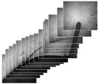
Figure 1 presents the generation of a mosaic from our underwater test environment. This mosaic was cre-ated using one robot and ASKF to estimate mosaic frames and robot positions. An Athlon XP 2400 with 512 MB of RAM memory was used to construct this mosaic and run-ning simulations.

4.2. LOCALIZINGMULTI-AUVS USINGASKF

We have developed an ASKF system able to receive as input the observation of the world: displacement between consecutive frames (zadj) and crossover regions (zcross), giving as output the prediction state (localization) of each robot and mosaic frames.

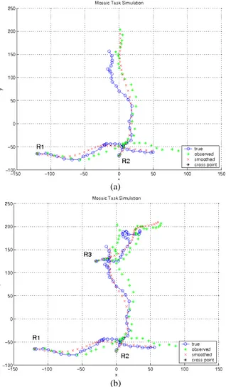
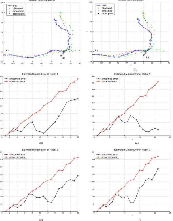
4.2.1. Two robots in a inspection task: We have

tested our system in a inspection simulated task with two

Figure 1. The visual map composed by a set of frames

robots: R1andR2. R1begins at (-120:-65) coordinates andR2begins at (0:-70) position, see figure 2(a). Each vehicle has a different dynamical model. Their percep-tion systems have different noise features. Circular points represent the true trajectory of each robot. In addition to real trajectory, the simulator gives the estimated trajec-tory provided by the perception system without crossover detection, it means only observed information (see star green points). We can see that we have a cumulative er-ror associated with the image processing observation (star points). Cross points show the smoothed trajectory ob-tained with our approach. We can see that, before the crossover both robots have a cumulative error between the real and estimated trajectories (see figure 2(b) and (c)). WhenR1crosses an old mosaic area imaging byR2(near (6:-49) coordinates), the ASKF provides a new estimation motion to R1, reseting its cumulative localization error (see 2(e)).

OnceR2has a lower cumulative localization error, it is used as setpoint. Therefore this robot holds the same old trajectory (and localization) after the crossover detec-tion, see figure 2(d) and (f).

Figure 3(a) shows the final estimated position at the end of this mission.

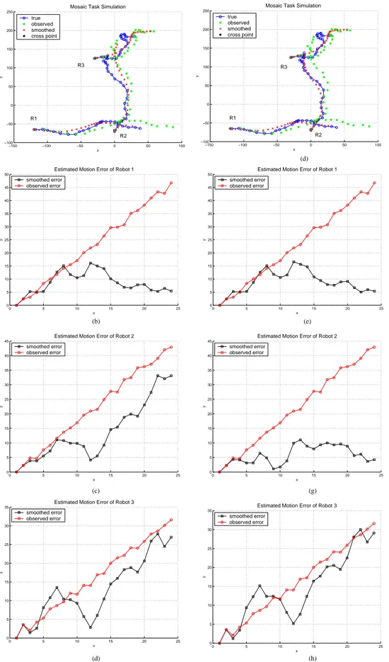
4.2.2. Three robots in a inspection task: We have

added a third robot, R3to the context. R3 begins at (-30:125), see figure 4(a). Now during the inspection there is another crossover situation, near (-11.8:125.6), provid-ing a second smoothed crossover correction in the final mosaic. It happens betweenR3andR2.

(7)

tra-(b) (a)

Figure 3. The simulated multi-AUV mosaicking with ASKF: (a) with 2 robots. (b) with 3 robots

.

jectory (and localization), see 4(d)(h). However,R2has an enhancement of its estimated localization, see 4(c)(g). Moreover, as ASKF updates all states of the system, and

R1 has an old intersection situation with R2, the for-mer suffers also a very small correction in its states, see 4(b)(f). The final mosaic and robot trajectories can be seen in figure 3(b).

Tables 1 and 2 show the final localization errors of both tests with 2 robots and 1 crossover situation and with one more robot and one more crossover situation. Sec-ond column shows the error between real and observed trajectory. Column 3 shows the error between real and ASKF corrected smoothed trajectory. Table 1 shows a decrease of around 93% of the estimation error ofR2 af-ter one crossover detection. In table 2, we can see that the final smoothed error decreases with two crossover situa-tions. With our approach, the localization mean errors of

Observed Error Smoothed Error

R1 51.8 3.8

R2 49.5 41.0

R3 -

-Table 1. Final errors with 2 robots and 1 crossover situations.

Observed Error Smoothed Error

R1 51.8 2,2

R2 49.5 7.5

R3 35 32.84

Table 2. Final errors with 3 robots and 2 crossover situations.

two robotsR1andR2have fallen by more than 85%.R3

mean error has not changed. As expected, the approach gives good results when a crossover situation between two robots happens when one of the robots is in the beginning of its trajectory, what means when one of the robots has a minor cumulative error.

Observe that the localization system workload is dis-tributed among the robots. Each robot can run its own ASKF, measuring its own frame adjacent displacement (zadj). It is necessary a centralized process only when a crossover risk exists. In this moment, a centralized crossover measure (zcross) must be calculated. The fleet shares information aiming to enhance individual localiza-tion estimative.

5. C

ONCLUSION

We have proposed and discussed a theoretical scheme for cooperative multi-AUVs Mosaicking. A set of robots can explore the seabed in a more efficient and faster way than a single vehicle. We have built a generic architecture for multi-robot cooperation. Its interest stems from its ability to provide a framework for cooperative decisional processes at different levels: mission decomposition and high level plan synthesis, task allocation and task achieve-ment.

(8)

R

EFERENCES

[1] R. Alami and S. S. C. Botelho. Plan-based multi-robot cooperation. In Michael Beetz, Jachim Hertzberg, Malik Ghallab, and Martha E. Pollack, editors, Advances in Plan-Based Control of Robotic Agents, volume 2466 of Lecture Notes in Computer Science. Springer, 2002.

[2] D Blidberg. The development of autonomous un-derwater vehicles (auvs); a brief summary. In IEEE Int. Conf. on Robotics and Automation (ICRA’01), 2001.

[3] S. S. C. Botelho, R. Mendes, L. Taddei, and M. Teix-eira. Lambdari um robô subaqüático autônomo. In Simpósio Brasileiro De Automação Inteligente - VI SBAI, 2003.

[4] R. Deaves. Covariance bounds for augmented state kalman filter application. IEEE Electronics Letters., 35(23):2062–2063, 1999.

[5] S. Fleischer. Bounded-error vision-based of au-tonomous underwater vehicles. PhD thesis, Stanford University, 2000.

[6] R Garcia. A Proposal to Estimate the Motion of an Underwater Vehicle Through Visual Mosaicking. PhD thesis, Universitat de Girona, 2001.

[7] R. Garcia, J. Puig, P. Ridao, and X. Cufi. Augmented state kalman filtering for auv navigation. In IEEE Int. Conf. on Robotics and Automation (ICRA’02), 2002.

[8] M.G. González, P. Holifield, and M. Varley. Im-proved video mosaic construction by accumulated alignment error distribution. In British Machine Vi-sion Conference, pages 377–387, 1998.

[9] R. Madhavan, K. Fregene, and L. Parker. Dis-tributed heterogeneous outdoor multi-robot localiza-tion. In IEEE Int. Conf. on Robotics and Automation (ICRA’02), 2002.

[10] H. Madjidi and S. Negahdaripour. On robustness and localization accuracy of optical flow computa-tion from color imagery. In 2nd Internacomputa-tional Sym-posium on 3D Data Processing, Visualization and Transmission, 2004.

[11] A. Matos and N. Cruz. Auv navigation and guid-ance in a moving acoustic network. In IEEE Oceans 2005, 2005.

[12] S. Roumeliotis and G. Bekey. Distributed multi-robot localization. IEEE Trans. on Robotics and Au-tomation, 18(5), 2002.

[13] Y. Rzhanov, L. M. Linnett, and R Forbes. Underwa-ter video mosaicing for seabed mapping. In InUnderwa-terna- Interna-tional Conference on Image Processing, 2000.

[14] A. Tavares. Um estudo sobre a modelagem e o con-trole de veículos subaquáticos não tripulados. Mas-ter’s thesis, Engenharia Oceânica,Fundação Univer-sidade Federal do Rio Grande, 2003.

[15] H Thomas. Advanced techniques for underwater vehicles positioning guidance and supervision. In IEEE Oceans 2005, 2005.

[16] A. Vargas, C.A. Madsen, and S. S. C. Botelho. Nav-ision - sistema de visão subaqüático para navegação e montagem de mosaicos em auvs. In Seminário e Workshop em Engenharia Oceânica, 2004.

(9)

−120 −100 −80 −60 −40 −20 0 20 40 −100

−50 0 50 100 150 200

x

y

Mosaic Task Simulation

true observed smoothed cross point

R1

R2

−120 −100 −80 −60 −40 −20 0 20 40 60

−100 −50 0 50 100 150 200

x

y

R1

R2

0 2 4 6 8 10 12 14 16 18 20

0 5 10 15 20 25 30 35 40

x

y

Estimated Motion Error of Robot 1

smoothed error observed error

0 5 10 15 20 25

0 5 10 15 20 25 30 35 40 45

x

y

0 5 10 15 20 25

0 5 10 15 20 25 30 35 40

x

y

0 2 4 6 8 10 12 14 16 18 20

0 5 10 15 20 25 30 35 40

x

y

(d)

(e)

(c) (f)

(b)

Figure 2. Inspection task with 2 robots and a crossover situation: The fleet localization before (a) and after the crossover detection (d). The error between true and both observed (in red) estimated (in black) trajectory of the robots before (b), (c) and after (e), (f) crossover detection.

(10)

−150 −100 −50 0 50 100 −100

−50 0 50 100 150 200 250

x

y

R1

R2 R3

−150 −100 −50 0 50 100

−100 −50 0 50 100 150 200 250

x

y

R1

R2 R3

0 5 10 15 20 25

0 5 10 15 20 25 30 35 40 45 50

x

y

0 5 10 15 20 25

0 5 10 15 20 25 30 35 40 45 50

x

y

0 5 10 15 20 25

0 5 10 15 20 25 30 35 40 45

x

y

0 5 10 15 20 25

0 5 10 15 20 25 30 35 40 45

x

y

0 5 10 15 20 25

0 5 10 15 20 25 30 35

x

y

0 5 10 15 20 25

0 5 10 15 20 25 30 35

x

y

(d)

(c) (b)

(h) (d)

(e)

(g)

Figure 4. Inspection task with 3 robots and 2 crossover situations: The estimated localization before (a) and after the crossover detection (e). The error between true and estimated trajectory of the robots before (b), (c) (d) and after (f), (g), (h) crossover detection.