case study approach
S. A. Christopher
Department of Atmospheric Science, The University of Alabama in Huntsville, Huntsville, AL, USA
Correspondence to:S. A. Christopher ([email protected])
Received: 25 March 2013 – Published in Atmos. Chem. Phys. Discuss.: ACPD 12 July 2013 Revised: 23 January 2014 – Accepted: 11 February 2014 – Published: 1 April 2014
Abstract.In anticipation of the upcoming GOES-R launch we simulate visible and near-infrared reflectances of the Ad-vanced Baseline Imager (ABI) for cases of high aerosol loading containing regional haze and smoke over the east-ern United States. The simulations are performed using the Weather Research and Forecasting (WRF), Sparse Matrix Operator Kernel Emissions (SMOKE), and Community Mul-tiscale Air Quality (CMAQ) models. Geostationary, satellite-derived, biomass-burning emissions are also included as an input to CMAQ. Using the CMAQ aerosol concentrations and Mie calculations, radiance is computed from the discrete ordinate atmospheric radiative transfer model. We present detailed methods for deriving aerosol extinction from WRF and CMAQ outputs. Our results show that the model simu-lations create a realistic set of reflectances in various aerosol scenarios. The simulated reflectances provide distinct spec-tral features of aerosols which are then compared to data from the Moderate Resolution Imaging Spectroradiometer (MODIS). We also present a simple technique to synthe-size green band reflectance (which will not be available on the ABI), using the model-simulated blue and red band re-flectance. This study is an example of the use of air quality modeling in improving products and techniques for Earth-observing missions.
1 Introduction
The Geostationary Operational Environmental Satellites-R Series (GOES-R) is the next generation of geostationary satellites that will offer a continuation of current products and services and enable new and improved applications (Schmit et al., 2005). The Advanced Baseline Imager (ABI) on
GOES-R (currently scheduled for 2016) will monitor clouds, aerosols, and surface features with a greater number of spec-tral bands and improved spatial resolutions when compared to the current GOES sensors (Schmit et al., 2008). The ABI will provide data in 16 spectral bands in the visible (0.47 and 0.64 µm), near-infrared (0.87, 1.38, 1.61, and 2.25 µm) and infrared (3.9, 6.19, 6.95, 7.34, 8.5, 9.61, 10.35, 11.2, 12.3, and 13.3 µm) portions of the electromagnetic spectrum. These improvements will help data assimilation and numer-ical weather prediction (NWP) applications, especially by providing crucial observations for regional and mesoscale data assimilations and predictions (Schmit et al., 2005).
Among the variety of application possibilities, GOES-R will also be used to monitor aerosols from fires and dust storms. The capabilities of GOES-R for air quality can cur-rently be assessed by simulating what GOES-R ABI would see when it is in orbit. The synthetic radiance computations require inputs for meteorological and chemical species fields and could be obtained from air quality models (e.g., WRF-CMAQ or WRF-CHEM).
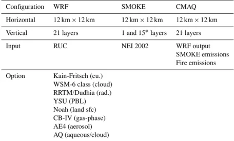
Table 1.Model inputs and configurations.
Configuration WRF SMOKE CMAQ
Horizontal 12 km×12 km 12 km×12 km 12 km×12 km Vertical 21 layers 1 and 15∗layers 21 layers
Input RUC NEI 2002 WRF output SMOKE emissions Fire emissions
Option Kain-Fritsch (cu.) WSM-6 class (cloud) RRTM/Dudhia (rad.) YSU (PBL) Noah (land sfc) CB-IV (gas-phase) AE4 (aerosol) AQ (aqueous/cloud)
∗Point emission sources.
to SBDART, which generates radiance and reflectance values for the GOES-R ABI bands.
This study examines the three cases in the eastern United States for high-aerosol-loading events including haze and fires. We compared the simulated surface PM2.5 mass
con-centrations with ground-based observations to assess the model performance. The model-simulated RGB imagery is also compared with the Moderate Resolution Imaging Spec-troradiometer (MODIS) data. From the perspective of spec-tral signature of various features, we present a simple tech-nique to synthesize green band reflectance, which will not be available on ABI. We show the synthetic RGB imagery that is produced based on the red, green (synthesized), and blue band reflectance.
2 Overview of case studies
The GOES-R ABI imagery is simulated for three cases in the eastern United States in 2008, 2010, and 2011.
2.1 Smoke in North Carolina on 10 June 2008
The Evans Road fires in North Carolina produced intense smoke, which circulated along the Mid-Atlantic coast on 10 June (shown as the red oval in the left panel of Fig. 1). Due to the semi-permanent Bermuda High weather system, regional haze was also visible along the eastern coastline of the United States. PM2.5 levels were also mostly
“moder-ate” to “unhealthy for sensitive groups” in this area (http: //airnow.gov).
2.2 Haze in Southeast on 8 July 2010
A large area of thick aerosol covered much of the Ohio Val-ley and the eastern portion of the United States. Smoke
con-tribution to this area of aerosol was not significant (middle panel of Fig. 1). The daily peak Air Quality Index (AQI) was reported between “moderate” to “unhealthy for sensitive groups” (http://airnow.gov).
2.3 Regional fires in Florida on 25 March 2011
There were numerous fires in the southern part of the United States. Observers reported fires and smoke in Kansas, Oklahoma, Texas, Missouri, Arkansas, Mississippi, Al-abama, Georgia, Florida, South Carolina, and North Car-olina. MODIS Aqua true color image (right panel of Fig. 1) showed smoke from several of the fires in Mississippi, Al-abama, Georgia, and Florida. These fires were agricultural (Mississippi and Alabama) and wildfires (near the boundary of Georgia and Florida).
3 Modeling approach
The WRF, CMAQ, and SBDART models in this study are at 12 km spatial resolution. For comparison purposes, we will show the model simulations at 19:00 UTC, at or near the MODIS Aqua overpass time.
3.1 WRF-SMOKE-CMAQ
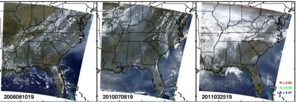
Fig. 1.MODIS Aqua imagery shows smoke from the Evans Road fire in North Carolina on 10 June 2008 (left), haze in Ohio Valley and Southeast on 8 July 2010 (middle), and agricultural fires and wildfires in Louisiana, Mississippi, Alabama, Georgia, and Florida on 25 March 2011 (right). The areas covered by plumes are shown as the red ovals. The imagery is available from http://www.star.nesdis.noaa. gov.
3.2 SBDART
SBDART is designed for the analysis of a wide variety of radiative transfer problems encountered in satellite remote sensing. It is based on a collection of reliable physical mod-els, which have been developed by the atmospheric science community over the past few decades (Ricchiazzi et al., 1998). The radiative transfer equation is numerically inte-grated with DISORT, where the discrete ordinate method provides a numerically stable algorithm to solve the equa-tions of plane-parallel radiative transfer in a vertically inho-mogeneous atmosphere (Stamnes et al., 1988). The intensity of both scattered and thermally emitted radiation can be com-puted at different heights and directions (Ricchiazzi et al., 1998).
SBDART requires several user-defined input files. For this study, we provide cloud and atmospheric conditions from WRF; aerosol loadings from CMAQ; aerosol diame-ter growth factor as a function of relative humidity for each aerosol type; surface albedo from the MODIS surface prod-uct (MCD43B3, containing both black sky and white sky albedos); spectral response function of the GOES-R ABI; and sun-satellite viewing geometry for GOES-R (solar zenith angle, viewing zenith angle). Optical Properties of Aerosols and Clouds (OPAC) (Hess et al., 1998) is also a useful re-source for refractive index and diameter growth factor for CMAQ aerosol species. Water and ice clouds are treated as spheres and for ice this is merely an approximation but note that this study is only focused on haze events. Aerosol opti-cal properties are assumed to be constant for each GOES-R ABI band. The procedures to compute spectral extinction are outlined in Appendix A.
4 Model results
4.1 Comparison of the measured and simulated surface PM2.5
Although one of the goals of this study is to simulate the radiance that the GOES-R ABI will observe, we are also in-terested in surface PM2.5mass concentrations to assess how
realistically the model calculates the mass concentration of aerosols.
Figure 2 compares the daily PM2.5 mass concentrations
from simulations and measurements at the AIRNow sta-tions on 10 June 2008, 8 July 2010, and 25 March 2011. The domain average PM2.5 concentrations are about 8.9
and 11.4 µg m−3 for the measured and simulated cases
re-spectively. The simulated PM2.5 is slightly biased toward
high concentration values because the majority of PM2.5
mass resides in the boundary layer, and the model often un-derestimates the nocturnal planetary boundary layer height (e.g., Yang et al., 2011). The PM2.5 mass concentrations
in Fig. 2 range from “Good” (0–15 µg m−3), “Moderate” (16–40 µg m−3) to “Unhealthy for Sensitive Groups” (41– 65 µg m−3)according to the AQI categories. The model per-formance for PM2.5 is consistent with the previous
stud-ies using the WRF-CMAQ and Eta-CMAQ over the eastern United States (Yu et al., 2012).
4.2 GOES-R reflectance
SBDART computes upward radiance and downward irradi-ance at the top of atmosphere (TOA). We convert them to reflectance for visualization (values from 0 to 1) and for in-terpretation purposes. Reflectance is defined as the ratio of the radiant flux reflected by a medium to that incident upon it. Therefore, spectral reflectance at TOA is given by
Fig. 2.Comparison of the simulated daily PM2.5mass concentra-tions with the measured at the AIRNow staconcentra-tions for 10 June 2008, 8 July 2010, and 25 March 2011.
whereRλ,Iλ, andFλare spectral reflectance (unitless),
spec-tral radiance (W m−2µm−1sr−1), and spectral irradiance of the sun (W m−2µm−1)at TOA, respectively. The quantity (π·Iλ) represents total upward radiant flux andθdenotes the
solar zenith angle (◦). Since the ABI filters reduce the appar-ent scene radiance and solar flux, reflectance should be unfil-tered to produce the reflectance measured by GOES-R ABI at TOA. The unfiltered ABI spectral reflectance is computed as
Rλ=
π·Rλλ12Sλ I λ dλ cosθ·Rλλ12Sλ F λ dλ
,
where Sλ is the spectral response of each ABI band. λ1
andλ2 are the cutoff wavelengths beyond which filter
re-sponse is assumed zero. We set the cutoff wavelengths atλo±0.5·FWHM, where λo and FWHM are the central
wavelength and full width at half maximum. The spectral response is assumed as Gaussian Boxcar Hybrid (GBH), where the top of the curve is flattened (data available at ftp://ftp.ssec.wisc.edu/ABI/SRF).
4.3 True color imagery derived from WRF-CMAQ-SBDART
To produce MODIS-like RGB images, we build a “synthetic” ABI filter for the green band that has a central wavelength at 0.55 µm and FWHM of 0.02 µm. The FWHM is assumed to be the same as that of the blue band, in the same manner as the MODIS blue and green bands.
The SBDART along with inputs from WRF-CMAQ are used to compute radiance and solar irradiance at TOA. The radiance and irradiance are converted to reflectance at
the ABI blue, green (assumed), and red bands. To obtain clearer, less hazy images, we do not include the Rayleigh scattering contribution in the SBDART runs, which can be called “Rayleigh corrected” in terms of remote sensing. The ocean-water-BRDF options include bio-pigments, foam, and sunglint reflectance of sea surface (see Vermote et al., 1997) with the default values of salinity=34 ‰, chlorin-ity=19 ‰, and wind speed=5 m s−1. Therefore, the TOA reflectance over ocean is primarily from scattering due to aerosols, foam, and white caps. Figure 3 shows the RGB ages produced from the simulations for GOES-R. The im-ages could be slightly different from the scenes visible to the human eyes because the ABI and our eyes differ in their spectral response. Another reason for this is the color im-age in Fig. 3 follows the imim-age enhancement scheme used by the MODIS Rapid Response team (http://earthdata.nasa. gov/data/near-real-time-data/rapid-response). The model-derived image is the one supposed to be measured from the GOES-R ABI. They are not directly comparable to the MODIS true color imageries because of the difference in viewing geometry between MODIS and GOES-R.
The cloud, aerosol, land, and ocean are well simulated in these images (Fig. 3); although, there is a need for improved cloud representation in dynamical models (Pour-Biazar et al., 2007). The clouds often differ from their positions in the simulated images due to difficulty in simulating the ob-served clouds from WRF. The model does not reproduce the small scale convective clouds during summer, especially on 8 July 2010, which is a topic for further investigation. The smoke aerosols on 10 June 2008 (Fig. 1, left) are spread more evenly along the mid-Atlantic coast (Fig. 3, left). This also happens to the plumes from the wildfires in the southern Georgia simulations on 25 March 2011, where plumes at two separate locations (Fig. 1, right) are viewed as one combined plume in the simulation (Fig. 3, right). The simulated haze on 8 July 2010 is seen in the eastern states (Fig. 3, middle), where the haze in Illinois, Indiana, and Kentucky was not ap-parent because of clouds in Fig. 1 (middle). It is shown that the simulations can capture the ocean color in the coastline of the Bahamas and around Key West. The model simulations are at 12 km spatial resolution where the surface consists of different land use types such as water, soil, trees, grasses, and so on. Thus, the simulated land surface scene may represent the mixture of different land use.
5 Synthetic RGB imagery
Fig. 3.The simulated RGB imagery viewed from GOES-R on 10 June 2008 (left), 8 July 2010 (middle), and 25 March 2011 (right).
using the red and blue bands, keeping in mind that this is only an approximation.
5.1 Spectral signatures
The spectral reflectance provides a valuable tool for differ-entiating features in images generated from solar reflectance bands. Under traditional classification schemes, supervised or unsupervised approaches identify key classes using dis-tinctive spectral signatures of each of the classes (Richards, 2012). The ground truth verifies the classification classes. However, in this study, classification can be done a priori using the model outputs (land cover, aerosol optical thick-ness, water/ice path, etc.). The classes identified by model re-sults, which we call “simulated truth”, can instead be used for spectral signature identification of constituent classes. These model-based spectral signatures may provide useful informa-tion about optimal selecinforma-tion of spectral bands by evaluating which band information is relevant or redundant for a given application.
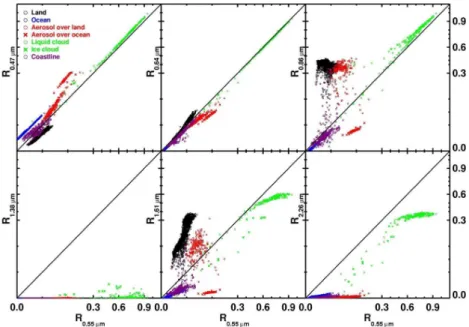
We select a representative set of pixels for land, ocean, aerosol, cloud, and coastline to view their spectral responses. Based on a priori knowledge, Table 2 shows the classifica-tion criteria in this study in which pixels are identified using the WRF and CMAQ outputs. Figure 4 shows the model-simulated spectral signatures of land, ocean, aerosol, and cloud. The reflectance range and average are shown with dots and a filled circle for each class. The simulated reflectance values at the green band are also included in Fig. 5 to com-pare them with the values at the other bands. The averaged green band reflectance lies between the averaged blue and red band reflectance. Figure 4 shows the reflectance at 1.38 µm is affected by water absorption, generating discernible response of ice cloud to the background land, ocean, and aerosol (King et al., 1992). The cloud and aerosol reflectance depends on cloud and aerosol optical thickness so that the spectral re-flectance range of cloud and aerosol shown in Fig. 4 could be changed by the classification selection rules in Table 2. The ocean generally has low reflectance, peaking in blue and decreasing as wavelength increases. Turbid water increases the reflectance in the red portion of the spectrum.
Fig. 4.Spectral signatures of land, ocean, aerosol, and cloud for 10 June 2008 (top), 8 July 2010 (middle), and 25 March 2011 (bot-tom). The spectral signatures for the imaginary green band are also shown between the blue and red bands.
Table 2.Classification criteria.
Class Classification criteria
Land LWP <0.001, FWP < 0.001, AOT < 0.02, and mask=land Ocean LWP < 0.001, FWP < 0.001, AOT < 0.02, and mask=ocean Aerosol over land LWP < 0.001, FWP < 0.001, AOT >0.15, and mask=land Aerosol over ocean LWP < 0.001, FWP < 0.001, AOT >0.15, and mask=ocean Cloud water LWP >200, FWP < 0.001, and AOT < 0.02
Cloud ice LWP < 0.001, FWP >800, and AOT < 0.02
Coastline LWP < 0.001, FWP < 0.001, AOT < 0.02, and mask=coastline LWP (Liquid Water Path) in g m−2from WRF, FWP (Frozen Water Path) in g m−2from WRF, AOT (Aerosol
Optical Thickness) from CMAQ.
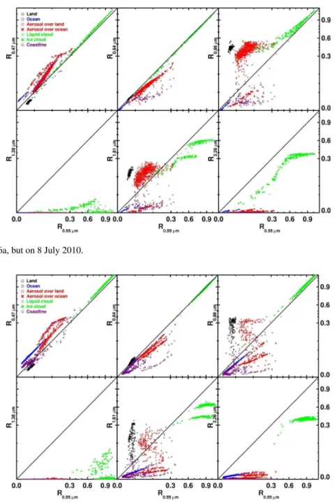
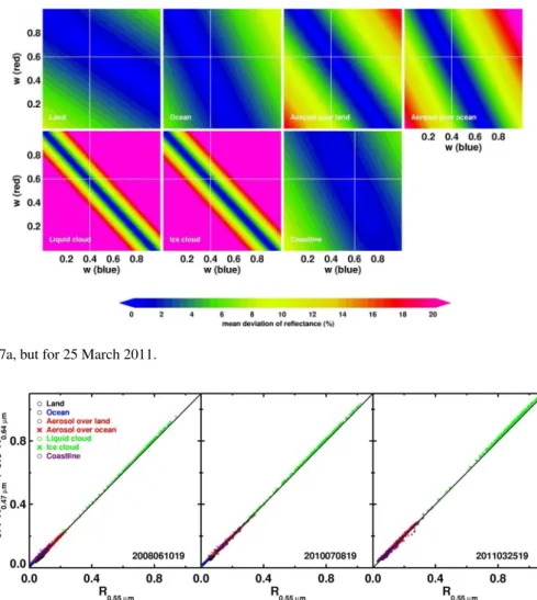
Fig. 5a.Plot of reflectance at the visible and near-IR bands against reflectance at the green band at 19:00 UTC, 10 June 2008. The Spectral signatures are shown for land, ocean, aerosol (over land and ocean), cloud (water and ice), and coastline. Note that the reflectance interval of 0.0 to 0.3 is enlarged to show more details of signatures from land, ocean, aerosol, and coastline.
5.2 Synthetic green band reflectance
The green band can be approximated using a look-up-table (LUT) approach, either using the MODIS blue, red, and IR bands (Miller et al., 2012) or using the blue, red, and near-IR band simulations from a radiative transfer model (Hillger et al., 2011). Both these approaches indicate that the synthe-sized green band imagery agrees with the observed MODIS or simulated green, reporting a less-green bias in the synthe-sized green values.
Miller et al. (2012) assume that the green band reflectance for each scene is a function of the red, blue, and near-IR (0.86 µm) bands. They generate scene-dependent green band LUTs from the MODIS red, blue, and near-IR bands. Once the ABI red, blue, and near-IR band reflectance were given, the green band reflectance is selected for the pair of the red-blue-near IR reflectance that makes the best match between the MODIS and ABI. This LUT approach would produce
the MODIS green band reflectance, not the GOES-R ABI reflectance. We expect slightly different spectral signatures of scenes between the MODIS and ABI because they have different filter spectral response and viewing geometries.
In contrast, Hillger et al. (2011) compute radiances at 0.47 µm (blue), 0.64 µm (red), and 0.865 µm (near-IR) us-ing a radiative transfer model along with the regional atmo-spheric modeling system (RAMS) outputs and the MODIS surface albedo product. The green band imagery is approx-imated from the blue, red, near-IR band simulations using the LUT method and compared with the directly-simulated green band imagery.
Fig. 5b.Same as in Fig. 6a, but on 8 July 2010.
Fig. 5c.Same as in Fig. 6a, but on 25 March 2011.
cloud, and “coastline”. The aerosol and cloud are further sep-arated into two classes in Table 2. For example, aerosols over land and ocean show different spectral behavior because coarse mode particles (dominated by sea salt) increase over ocean. Similarly, liquid cloud is distinguished from ice cloud due to the differences in the imaginary part of their refrac-tive index. Figure 5 shows the ice cloud can be discriminated from the liquid cloud using the visible (0.55 µm or 0.64 µm), and near-IR (1.38 µm or 1.61 µm) (e.g., Schmidt et al., 2005; Baum et al., 2005).
This study focuses on synthesizing the green band re-flectance as a function of rere-flectance at visible and near-IR bands. Figure 5 shows the relationships between the green and other band reflectance for each class. As expected, the classes show complex spectral responses of reflectance. Surprisingly, strong linear relationships are found between R0.47 µmandR0.55 µm(top left in Fig. 5) and betweenR0.64 µm
andR0.55 µm(top middle in Fig. 5) for all classes specified in
Table 2, whereR0.47 µm,R0.55 µm, andR0.64 µmare reflectance
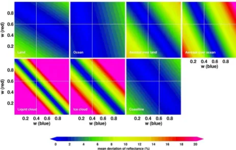
Fig. 6a.Mean difference between the synthesized and simulated green band reflectance with varyingwBandwRfor land, ocean, aerosol
(over land and ocean), cloud (liquid and ice), and coastline for 10 June 2008. The unit is reflectance in percent. The point atwB=0.4 and
wR=0.6 is shown for land, ocean, aerosol, and cloud. The point atwB=0.6 andwR=0.6 is also shown for coastline.
Fig. 6b.Same as in Fig. 7a, but for 8 July 2010.
andR0.64 µmindicates that the blue, green, and red bands
con-tain redundant spectral information for cercon-tain classes. We expect thatR0.55 µmin a pixel can be estimated usingR0.47 µm
andR0.64 µm.
5.3 RGB imagery
A linear relationship betweenR0.55 µmandR0.64 µm(and
be-tweenR0.47 µm andR0.55 µm ) is not sufficient enough to
de-riveR0.55 µmfromR0.64 µmbecause the linear relationship
dif-fers from one class to another. Therefore, it is necessary to classify each scene before applying the linear relationship, although scene classification could be a challenging problem.
Alternatively, it is noted in Fig. 5 that green band reflectance can be approximated by one or two linear combinations of blue and red band reflectance for all classes.
The green band reflectance can be expressed as a sim-ple relation,Gsyn=wB·B+wR·R, whereGsyn,B, andR
are the synthesized green, simulated red, and simulated blue band reflectance, respectively. The coefficients,wBandwR,
give the weights of blue and red band reflectance in deter-mining green band reflectance. However, wB and wR
dif-fer for difdif-ferent classes, butwBandwRhave a range within
Fig. 6c.Same as in Fig. 7a, but for 25 March 2011.
Fig. 7.Comparison of the synthesized and simulated green band reflectance, where the synthesized green band reflectance is derived from the blue and red band reflectance. The coastline are produced with a different blue-red combination such asGsyn=0.6·B+0.6·R.
reflectance, where the synthesized reflectance is derived by Gsyn=wB·B+wR·R with varyingwBandwR. Since the
minima of reflectance difference occur over a range, not at a point, inwBandwRspace, we can select an optimal weight
pair whose reflectance difference is close to minimum for all classes.
After searching for optimalwBandwRpairs for three
dif-ferent days, we chose twowBandwRpairs, such that green
band reflectance is well approximated (synthesized) by the relations,
Gsyn=0.4·B+0.6·Rfor land,ocean,aerosol,and cloud
Gsyn=0.6·B+0.6·Rfor coastline
Figure 7 shows that the synthesized (Gsyn)and simulated
green band reflectance (G) are almost the same except for coastline. The relatively large uncertainty inGsynfor
coast-line was also recognized in the LUT method (Hillger et al., 2011; Miller et al., 2012). The synthesized green band re-flectance differs from the simulated by up to about 0.01 for
land, ocean, aerosol, and cloud and by 0.01–0.03 for coast-line.
The synthetic RGB imagery using the synthetic green band reflectance is shown in Fig. 8. The synthetic RGB imagery appears almost identical to the simulated one with subtle bi-ases. The ocean and cloud in the synthesized RGB imagery (Fig. 7) are slightly brighter (less than 0.01 in reflectance) than those in the simulated RGB imagery (Fig. 3).
We introduce an approach to synthesize RGB imagery while there is a missing green band in GOES-R ABI. This approach uses the synthesized green band reflectance that is derived by a simple relation of the red and blue band re-flectance, i.e.,Gsyn=0.4·B+0.6·R. Since the coastline
Fig. 8.Synthetic RGB imagery at 19:00 UTC, 10 June 2008 (left), 8 July 2010 (middle), and 25 March 2011 (right). The green band reflectance is synthesized from the simulated blue and red band reflectance using the relations,Gsyn=0.4·B+0.6·Rfor land, ocean,
aerosol, and cloud, andGsyn=0.6·B+0.6·Rfor coastline.
also possible to apply the equation,Gsyn=0.4·B+0.6·R,
to all classes although this simplest approach may cause a little more bias in coastline. The difference is probably neg-ligible considering the reflectance difference for coastline in Fig. 6 atwB=0.4 and 0.6. The approach shown in this
study is attractive for operational purposes because it pro-duces RGB imagery well, needs only simple calculations, and does not need a database for LUTs. While this approach is promising, more case studies need to be conducted to re-fine and confirm the methods and analysis.
6 Summary and discussion
The GOES-R ABI visible and near-infrared reflectance are simulated using WRF, SMOKE, CMAQ, and SBDART mod-els for cases of high aerosol loadings with haze and smoke over the eastern United States. The simulations reproduce the state of meteorological fields, background emissions, and chemical transport of air pollutants. To represent more real-istic scenarios, satellite-derived, biomass-burning emissions are also included as an input to CMAQ. The simulated RGB imagery appears realistic in various aerosol scenarios. We classify the model scenes by seven classes based on their spectral signatures at the 12 km spatial resolution. The green band reflectance is synthesized from red and blue bands. The resulting synthesized RGB images appear almost identical to the model-simulated ones.
This study examines the use of air quality modeling to simulate spectral signatures from various scenes. We show that the model-based spectral signatures provide a simple way to select relevant and to deselect irrelevant spectral in-formation from multispectral data. As an exercise, we syn-thesize true color imagery which perhaps appeals both to professional and inexperienced users of GOES-R products (Huff et al., 2012). We suggest that the green band re-flectance is synthesized by a simple relationship such as Gsyn=0.4·B+0.6·R, although the relationship can be
fur-ther improved with more case studies.
Acknowledgements. This research was sponsored by NOAA Air
Quality projects at UAHuntsville. PM2.5data were obtained from EPA’s Air Quality System (AQS). The author would like to thank his team members for their help with producing some of the figures.
Edited by: L. M. Russell
References
Baum, B. A., Heymsfield, A. J., Yang, P., and Bedka, S. T.: Bulk scattering properties for the remote sensing of ice clouds. Part I: Microphysical data and models, J. Appl. Meteorol., 44, 1885– 1895, 2005.
Binkowski, F. S. and Roselle, S. J.: Models-3 Community Multiscale Air Quality (CMAQ) model aerosol component 1. Model description, J. Geophys. Res.-Atmos., 108, 4183, doi:10.1029/2001JD001409, 2003.
Evans, B. T. N. and Fournier, G. R.: Simple approximation to ex-tinction efficiency valid over all size parameters, Appl. Optics, 29, 4666–4670, 1990.
Grell, G. A., Dudhia, J., and Stauffer, D. R.: A description of the Fifth-Generation Penn State/NCAR Mesocale Model (MM5), NCAR Technical Note, NCAR/TN 398+STR, Boulder, CO, 138, 1994.
Hess, M., Koepke, P., and Schult, I.: Optical Properties of Aerosols and Clouds: The Software Package OPAC, B. Am. Meteorol. Soc., 79, 831–844, doi:10.1175/1520-0477(1998)079<0831:OPOAAC>2.0.CO;2, 1998.
Hillger, D., Grasso, L., Miller, S., Brummer, R., and DeMaria, R.: Synthetic advanced baseline imager true-color imagery, J. Appl. Remote Sens., 5, 053520, doi:10.1117/1.3576112, 2011. Houyoux, M. R., Vukovich, J. M., Coats Jr, C. J., Wheeler, N. J.
Pour-Biazar, A., McNider, R. T., Roselle, S. J., Suggs, R., Jedlovec, G., Byun, D. W., Kim, S., Lin, C. J., Ho, T. C., Haines, S., Dornblaser, B., and Cameron, R.: Correcting photolysis rates on the basis of satellite observed clouds, J. Geophys. Res., 112, D10302, doi:10.1029/2006JD007422, 2007.
Ricchiazzi, P., Yang, S., Gautier, C., and Sowle, D.: SBDART: A Research and Teaching Software Tool for Plane-Parallel Radia-tive Transfer in the Earth’s Atmosphere, B. Am. Meteorol. Soc., 79, 2101–2114, 1998.
Richards, J.: Remote Sensing Digital Image Analysis, An Intro-duction, Springer, Fifth Edn., Springer-Verlag, Germany, 494 pp, 2012.
Schaaf, C. B., Gao, F., Strahler, A. H., Lucht, W., Li, X., Tsang, T., Strugnell, N. C., Zhang, X., Jin, Y., Muller, J.-P., Lewis, P., Barnsley, M., Hobson, P., Disney, M., Roberts, G., Dunderdale, M., Doll, C., d’Entremont, R. P., Hu, B., Liang, S., Privette, J. L., and Roy, D.: First operational BRDF, albedo nadir reflectance products from MODIS, Remote Sens. Environ., 83, 135–148, doi:10.1016/s0034-4257(02)00091-3, 2002.
Optics, 27, 2502–2509, 1988.
Vermote, E. F., Tanré, D., Deuzé, J. L., Herman, M., and Morcrette, J. J.: Second simulation of the satellite signal in the solar spec-trum, 6s: an overview, IEEE T. Geosci. Remote, 35, 675–686, 1997.
Yang, E.-S., Christopher, S. A., Kondragunta, S., and Zhang, X.: Use of hourly Geostationary Operational Environmen-tal Satellite (GOES) fire emissions in a Community Multi-scale Air Quality (CMAQ) model for improving surface par-ticulate matter predictions, J. Geophys. Res., 116, D04303, doi:10.1029/2010jd014482, 2011.
Yu, S., Mathur, R., Pleim, J., Pouliot, G., Wong, D., Eder, B., Schere, K., Gilliam, R., and Rao, S. T.: Comparative evaluation of the impact of WRF/NMM and WRF/ARW meteorology on CMAQ simulations for PM2.5and its related precursors during
Appendix A
Calculation of spectral extinction from CMAQ outputs
From CMAQ outputs, we have the aerosol mass concentra-tions in µg m−3of aerosol species for Aitken, accumulation and coarse modes.
1. Convert mass concentrations of CMAQ aerosol species to volume in m3m−3.
2. Sum the volume over all species for Aitken, accu-mulation and coarse modes. This is possible since all species in each mode are assumed to have the same size distribution.
3. Calculate the geometric mean diameter (Dg) and
geometric mean standard deviation (σg) using the
Eqs. (5a) and (5b) of Binkowski and Roselle (2003). The standard deviation for coarse mode is constant at 2.2 (CMAQ source code assumption).
4. Evaluate the optical coefficients, including the effects of hydroscopic growth, since we have the wet state refractive index (m=n−ik) of each OPAC aerosol mode (inso, soot, waso, etc.). The relative humidity is obtained from the WRF outputs (water vapor mixing ratio, pressure, and air temperature). In order to get the wet radius (or diameter), we can use the fact that only the mean diameter changes and the growth fac-tor is universal as a function of RH. Therefore, we can writeD(wet)=g(RH)·D(dry), where the growth fac-tor, g(RH), can be determined by the ratios of the wet diameters to the dry diameters at RH=0, 50, 70, 80, 90, 95, 98, and 99 in % (see OPAC optdat for water soluble, sulfate, and sea salt).
5. Qext, the Mie extinction efficiency factor, is a function
of αand an index of refraction of the particles. It is calculated from the Evans and Fournier approximation (Evans and Fournier, 1990) for each CMAQ species. 6. The aerosol extinction coefficientbsp(km−1)must be
calculated from ambient aerosol characteristics as in-dex of refraction (m=n−ik), volume concentration and size distribution; at wavelengthλ,bsp(km−1)may
be expressed as (Binkowski and Roselle, 2003):
βsp=
3π 2λ Z ∞ −∞ Qext α dV d lnαd lnα
The particle distribution is given in a lognormal form as dV
d lnα=VT( A π)
1/2
exp[−Aln2(α αv
)]
whereα=π Dλ ,αv=π Dλg, and A= 1
2 ln2σg.VT is the total
particle volume concentration, andQext, the Mie extinction
efficiency factor as mentioned above.
If the water uptake effect is included, i.e., ambient envi-ronments are considered, the above equation becomes,
βsp=3π 2λ
Z ∞
−∞
Qext,amb αamb
dVamb
d lnαambd lnαamb= 3π 2λ
Z ∞
−∞
Qext,amb αdry
·g(RH)2· dVdry
d lnαdry
d lnαdry
=3π
2λ·g(RH)
2·V dry·(
1 2πln2σ
g
)(1/2)·Z∞
0
Qext,amb
α2 ·exp[−
1 2·
ln2(αα
v)
ln2σ g
] ·dα
where
αamb=g(RH)·αdry
dVamb
d lnαamb
=Vamb(
A π)
1/2
exp[−Aln2( αamb αv,amb
)]
= {Vdryg(RH)3}( A π)
1/2
exp[−Aln2( αdry αv,dry
)] =g(RH)3 dVdry d lnαdry
d lnαamb=
dαamb
αamb
=g(RH)·dαdry
g(RH)·αdry
=dαdry
αdry
=d lnαdry
d lnα=dαα andα→0 as lnα→ −∞ α→ ∞ as lnα→ +∞