www.clim-past.net/9/969/2013/ doi:10.5194/cp-9-969-2013
© Author(s) 2013. CC Attribution 3.0 License.
Climate
of the Past
Geoscientiic
Geoscientiic
Geoscientiic
Geoscientiic
The sensitivity of the Arctic sea ice to orbitally induced insolation
changes: a study of the mid-Holocene Paleoclimate Modelling
Intercomparison Project 2 and 3 simulations
M. Berger1,2, J. Brandefelt1,2, and J. Nilsson2,3
1Linn´e Flow Centre, Dept. of Mechanics, Royal Institute of Technology, Stockholm, Sweden 2Bert Bolin Centre for Climate Research, Stockholm University, Stockholm, Sweden 3Dept. of Meteorology, Stockholm University, Stockholm, Sweden
Correspondence to:M. Berger (marit@mech.kth.se)
Received: 17 July 2012 – Published in Clim. Past Discuss.: 13 August 2012 Revised: 28 February 2013 – Accepted: 14 March 2013 – Published: 15 April 2013
Abstract. In the present work the Arctic sea ice in the mid-Holocene and the pre-industrial climates are analysed and compared on the basis of climate-model results from the Paleoclimate Modelling Intercomparison Project phase 2 (PMIP2) and phase 3 (PMIP3). The PMIP3 models generally simulate smaller and thinner sea-ice extents than the PMIP2 models both for the pre-industrial and the mid-Holocene cli-mate. Further, the PMIP2 and PMIP3 models all simulate a smaller and thinner Arctic summer sea-ice cover in the mid-Holocene than in the pre-industrial control climate. The PMIP3 models also simulate thinner winter sea ice than the PMIP2 models. The winter sea-ice extent response, i.e. the difference between the mid-Holocene and the pre-industrial climate, varies among both PMIP2 and PMIP3 models. Ap-proximately one half of the models simulate a decrease in winter sea-ice extent and one half simulates an increase. The model-mean summer sea-ice extent is 11 % (21 %) smaller in the mid-Holocene than in the pre-industrial climate simula-tions in the PMIP2 (PMIP3). In accordance with the sim-ple model of Thorndike (1992), the sea-ice thickness re-sponse to the insolation change from the pre-industrial to the mid-Holocene is stronger in models with thicker ice in the pre-industrial climate simulation. Further, the analyses show that climate models for which the Arctic sea-ice re-sponses to increasing atmospheric CO2 concentrations are
similar may simulate rather different sea-ice responses to the change in solar forcing between the mid-Holocene and the pre-industrial. For two specific models, which are anal-ysed in detail, this difference is found to be associated with
differences in the simulated cloud fractions in the summer Arctic; in the model with a larger cloud fraction the effect of insolation change is muted. A sub-set of the mid-Holocene simulations in the PMIP ensemble exhibit open water off the north-eastern coast of Greenland in summer, which can pro-vide a fetch for surface waves. This is in broad agreement with recent analyses of sea-ice proxies, indicating that beach-ridges formed on the north-eastern coast of Greenland during the early- to mid-Holocene.
1 Introduction
minimum in the Arctic sea-ice cover in the Holocene be-tween 8.5 and 6 ka BP, and furthermore that during this pe-riod the region northeast of Greenland was ice-free in sum-mer (Funder et al., 2011; Jakobsson et al., 2010; Polyak et al., 2010). This remarkable finding is based on several inde-pendent sea-ice proxies including driftwood, bowhead whale fossils, and coastal erosion. At present, the thickest sea ice is encountered in the region north of Greenland, which could be taken to imply that the summer ice was completely lost in some intervals during the mid-Holocene. Another possi-ble explanation for the beach-ridges could be a change in the wind-pattern in the Arctic, possibly resulting in different cir-culation patterns than at present. This may be consistent with the occurrence of seasonally ice-free regions around the Arc-tic Ocean in the mid-Holocene (Funder et al., 2011). How-ever, the sea-ice reconstructions do not unequivocally sup-port this notion (e.g. de Vernal et al., 2008).
The notion that the Arctic Ocean could have lost all its summer ice in the mid-Holocene is of interest in the light of the observed current downward trend in the Arctic sea-ice cover. In the late 1970s the first satellites were launched, en-abling monitoring of the Arctic ice cover. The mean sea-ice extent during the period 1979–2000 ranged from a max-imum of 16 million km2in March to a September minimum of 7 million km2 (Serreze et al., 2007). The extent has de-clined since 1979, with the smallest extent (3.4 million km2) since 1979 observed in September 2012. The changes ob-served in the sea-ice extent since the late 1970s are mainly confined to the coasts of Alaska and Siberia, with smaller changes along the northern coast of Greenland and the Cana-dian Archipelago (Cavalieri et al., 2008). The reduction in sea-ice cover observed in recent years is most likely due to anthropogenic climate change (Notz and Marotzke, 2012). A reduction of the sea-ice thickness has also been observation-ally confirmed. The thinning of the ice is observed over the entire Arctic Ocean (Kwok and Rothrock, 2009; Rothrock et al., 2003), and mainly reflects a reduction of the thick multi-year ice. During the same period the increase in surface tem-perature in the Arctic region exceeded 2◦C, which is twice as much as the global average temperature increase (Solomon et al., 2007).
One road to improve the physical understanding of the Arctic sea ice and its response to future increases of the atmospheric greenhouse gas concentrations is to study the behaviour of the Arctic sea ice under climatic forcing conditions characterising past climate epochs. This gen-eral approach to climate research is adopted in the Paleo-climate Modelling Intercomparison Project (PMIP), which uses state-of-the-art climate models to simulate past cli-mates functionally different from the present-day climate. The focus of PMIP is both model-to-model comparison and model-to-data comparison (Braconnot et al., 2007a). Two of the periods that have been examined in-depth are the mid-Holocene (MH) warm period, approximately 6 ka BP, and the last glacial maximum (LGM), approximately 21 ka BP.
Previous studies of the PMIP data include an analysis of the large-scale features of the PMIP2 MH simulations (Braconnot et al., 2007a) and the high latitude heat budget Braconnot et al. (2007b). Both show a general MH warming in the Arctic in the Northern Hemisphere summer, stronger over continents than over ocean. Zhang et al. (2010) compare the PMIP2 models to available proxy-data, and show that the ocean–atmosphere–vegetation models generally fit bet-ter with data than the ocean–atmosphere models. They also find that some models have a strong warming in the Barents sea region during the winter months, despite a decrease in insolation, indicating that the sea-ice response in summer is important also for the winter temperature.
The focus of the present work is to analyse and compare the Arctic sea-ice extent and thickness in the mid-Holocene and pre-industrial (PI) PMIP simulations, using results from both the second and third-phase of the project (PMIP2 and PMIP3). The analysis includes a model-to-model compari-son and an investigation of the models’ response to the MH forcing, as well as a comparison of the PMIP2 and PMIP3 ensembles.
The PMIP models and experiments are described in more detail in Sect. 2. In Sect. 3 a simple thermodynamic model of Thorndike (1992), describing the melt and growth of the sea ice, is introduced and used to analyse the sea-ice thickness response to the change in insolation between MH and PI. The spatial patterns of sea-ice concentration, sea-ice thick-ness and surface temperature in both the PI simulation and the MH simulation are analysed in Sect. 4. Here we also consider the response in the seasonal variation of the sea-ice thickness in the warmer MH climate. The results are dis-cussed in Sect. 5 and the conclusions are presented in Sect. 6.
2 Models and experiments
2.1 Experimental design
The PMIP2 experiment was set up with a pre-industrial cli-mate (1750 AD clicli-mate), with orbital parameters of 1950 AD and trace gases corresponding to 1750 AD. The difference in solar insolation due to the change in orbital parameters from 1750 AD to 1950 AD is negligible (Braconnot et al., 2007a). The initial ocean state used for the PI experiment was mod-ern, and the initial salinity and ocean temperature was taken from the Levitus et al. dataset (1998). The PMIP3 PI experi-ments were identical to the Climate Modelling Intercompar-ison Project 5 (CMIP5) experiments, hence different defini-tions of greenhouse gases, the solar constant, land surface and orbital parameters were used by the modelling groups (Braconnot et al., 2011). The experimental set up for both the PMIP2 and PMIP3 mid-Holocene simulations followed the PMIP protocol (Braconnot et al., 2007a,b, 2011).
parameters. The orbital configuration in the MH climate re-sults in an increased summer and annual mean insolation in the Northern Hemisphere compared to the PI climate. In the MH PMIP2 and PMIP3 experiments the atmospheric CH4
concentration is 650 ppb. The atmospheric CH4
concentra-tion in the PMIP2 is 760 ppb, in the PMIP3 this concentraconcentra-tion varies among the models. The increased solar insolation dur-ing MH is more important in terms of radiative forcdur-ing than the reduction in CH4concentration (Braconnot et al., 2007a;
Renssen et al., 2009). The decreased global average radiative forcing at the top of the atmosphere due to a decrease of the atmospheric CH4 concentration from 760 to 650 ppb
corre-sponds to 0.07 W m−2(Otto-Bliesner et al., 2006), whereas the maximum increase in June insolation at 65◦N for the MH is 40 W m−2at the top of the atmosphere (Berger, 1978). For comparison, the globally averaged top of the atmosphere in-crease in radiative forcing due to a doubling of the present day atmospheric CO2concentration is 3.7 W m−2(Solomon
et al., 2007).
2.2 Models
The mid-Holocene and pre-industrial control simulations from 11 models form part of the PMIP2 ensemble and 12 models of the PMIP3 ensemble are included in this study. The PMIP2 data is available through the PMIP2 database (http://pmip2.lsce.ipsl.fr/). The PMIP3 data is available via the Program for Climate Model Diagnosis and Intercompar-ison (PCMDI).
The PMIP2 experiments were performed with the same model versions as used for future climate simulations per-formed for the Climate Modelling Intercomparison Project 3 (CMIP3), but in most cases the PMIP2 simulations were run at lower resolution (Braconnot et al., 2007a). Two modelling centres submitted simulations run with the same model ver-sion for both the CMIP3 and PMIP2 experiments. These are utilized for comparison of the response of the Arctic sea ice to MH forcing with the response to a 1 % per year increase to doubling of the atmospheric CO2 concentration. For the
PMIP3 models, the MH simulations are run with the same resolution and the same versions of the model as the historic and representative concentration pathway (RCP) future sce-narios in the CMIP5 ensemble.
The models included in this study are listed in Ta-ble 1. From the PMIP2 ensemTa-ble only the ocean–atmosphere global circulation models are considered here. These include sea-ice models of different complexity. Three of the PMIP2 models, FGOALS-1.0g, FOAM, and UBRIS-HadCM3M2, include only thermodynamic sea-ice models, the other 8 models have thermodynamic and dynamic sea-ice models. In the PMIP3 ensemble, all models have thermodynamic and dynamic sea ice models. In general, the PMIP3 models have more advanced representations of sea-ice-relevant physical processes. The majority of the PMIP3 models also include dynamic vegetation, which affects simulated temperature
response in the models (Zhang et al., 2010; Braconnot et al., 2007b).
The analysis is performed on monthly mean data from the last 100 model years submitted to the database, or over as many years as were available in the database. To facilitate model intercomparison, the model output was interpolated to a common regular (0.5◦×1◦) latitude–longitude grid using bilinear interpolation. Since the models have different grids and land mask, the remapping to the common grid can cause small biases in the calculated sea-ice extent.
3 Thermodynamic considerations
We will here use simple thermodynamic considerations to qualitatively examine the response of the Arctic sea-ice cover to the change in insolation between the pre-industrial era and the mid-Holocene. This insolation change is mainly at-tributed to changes in the precessional cycle and the obliquity cycle; the changes in eccentricity being essentially negligible (e.g. Pierrehumbert, 2010; Hartman, 1994). The precessional cycle chiefly involves a redistribution of the insolation over the season, whereas the obliquity cycle involves a redistribu-tion of the insolaredistribu-tion over the latitudes. In the high northern latitudes, the higher obliquity in the mid-Holocene resulted in higher summer insolation and slightly weaker winter inso-lation compared to the pre-industrial. Moreover in the mid-Holocene, the northern summer occurred when the Earth was close to perihelion, which yielded a higher peak in the sum-mer insolation. Together, these two effects yielded a mean June insolation at 65◦N that was about 40 W m−2stronger in the mid-Holocene than in the pre-industrial era. When the Earth is closest to the Sun in its orbit, however, Kepler’s sec-ond law implies higher orbital velocities and hence shorter summer seasons. As a result, the integrated insolation over the summer season hardly changes with the precessional cy-cle (Pierrehumbert, 2010).
3.1 Thorndike’s two-season ice model
We will now use the thermodynamic two-season ice model developed by Thorndike (1992) to estimate the ice thickness response due to orbitally induced changes in the insolation. The model approximates the annual cycle as one melt season, when the temperature of the ice is at the melting point, and one growing season. As discussed by Thorndike (1992), this is an idealization of the real seasonal temperature–thickness cycle of sea ice, which is illustrated in Fig. 1. In the model, described in detail by Thorndike (1992) and Bitz and Roe (2003) the ice meltingMand growthG, in meters, are given by
M=τM
L (−FLW+FW+(1−αi)FSW) , (1)
G(h)=τG
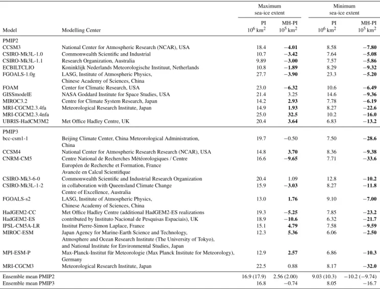
Table 1.Sea-ice extent in the month with minimum and maximum sea-ice extent for the PI and MH. A grid cell is considered covered with sea ice if the sea-ice concentration is larger than 15 %. The models with statistically significant changes between MH and PI are marked boldface. The ensemble mean for PMIP2 are excluding (including) FGOALS. All models simulate significantly reduced minimum sea-ice extents, and almost all simulate significant changes in the maximum extent.
Maximum Minimum
sea-ice extent sea-ice extent
PI MH-PI PI MH-PI
Model Modelling Center 106km2 105km2 106km2 105km2
PMIP2
CCSM3 National Center for Atmospheric Research (NCAR), USA 18.4 −4.01 8.58 −7.80
CSIRO-Mk3L-1.0 Commonwealth Scientific and Industrial 10.7 −3.42 7.64 −5.08
CSIRO-Mk3L-1.1 Research Organization, Australia 9.89 −3.00 7.57 −5.86
ECBILTCLIO Koninklijk Nederlands Meteorologische Instituut, Netherlands 10.8 −1.89 8.29 −9.32
FGOALS-1.0g LASG, Institute of Atmospheric Physics, 27.7 −3.90 23.3 −5.20
Chinese Academy of Sciences, China
FOAM Center for Climatic Research, USA 23.0 −6.32 10.6 −6.49
GISSmodelE NASA Goddard Institute for Space Studies, USA 21.4 3.25 14.6 −9.36
MIROC3.2 Centre for Climate System Research, Japan 14.2 2.93 7.78 −6.19
MRI-CGCM2.3.4fa Meteorological Research Institute, Japan 14.9 1.93 8.27 −22.6
MRI-CGCM2.3.4nfa 25.0 32.5 10.2 −16.0
UBRIS-HadCM3M2 Met Office Hadley Centre, UK 20.4 3.64 6.83 −13.2
PMIP3
bcc-csm1-1 Beijing Climate Center, China Meteorological Administration, 19.7 −0.50 7.50 −28.6
China
CCSM4 National Center for Atmospheric Research Research (NCAR), USA 14.8 3.70 8.36 −9.38
CNRM-CM5 Centre National de Recherches M´et´eorologiques / Centre 16.6 −9.65 7.71 −33.6
Europ´een de Recherche et Formation, France Avanc´ee en Calcul Scientifique
CSIRO-Mk3-6-0 Commonwealth Scientific and Industrial Research Organization 20.4 1.09 12.8 −10.2
CSIRO-Mk3L-1-2 in collaboration with Queensland Climate Change 15.9 −3.03 8.27 −11.8
Centre of Excellence, Australia
FGOALS-s2 LASG, Institute of Atmospheric Physics, 13.0 1.76 9.10 −7.00
Chinese Academy of Sciences, China
HadGEM2-CC Met Office Hadley Centre (additional HadGEM2-ES realizations 19.3 −5.25 7.85 −23.2
HadGEM2-ES contributed by Instituto Nacional de Pesquisas Espaciais), UK 18.9 −10.6 6.32 −21.7
IPSL-CM5A-LR Institut Pierre-Simon Laplace, France 15.1 4.79 7.58 −9.59
MIROC-ESM Japan Agency for Marine-Earth Science and Technology, 12.3 5.36 6.06 −2.50
Atmosphere and Ocean Research Institute (The University of Tokyo), and National Institute for Environmental Studies, Japan
MPI-ESM-P Max-Planck-Institut f¨ur Meteorologie (Max Planck Institute for Meteorology), 12.9 2.57 6.86 −10.3
Germany
MRI-CGCM3 Meteorological Research Institute, Japan 22.5 0.88 8.17 −32.0
Ensemble mean PMIP2 16.9 (17.9) 2.56 (2.00) 9.03 (10.3) −10.2 (−9.74)
Ensemble mean PMIP3 16.8 −0.74 8.05 −16.7
whereτM/τGis the length of the melt/growth season,Lthe latent heat of fusion,FLW the net upward flux of longwave
radiation,FWthe oceanic heat flux at the base of the ice,h
is the annual-mean ice thickness,αi the ice albedo. Further, FSW, the mean surface downward insolation over the melt
season, is defined by
FSW=(1−αa)
1 τM
toZ+τM
to
ˆ
FSW(t′)dt′, (3)
whereFˆSWis the downward shortwave radiation at the top
of the atmosphere andαa an effective atmospheric albedo,
which depends on the reflectivity and absorptivity of the at-mosphere as well as the surface albedo (see e.g. Donohoe and Battisti, 2011).
Based on observational results presented by Donohoe and Battisti (2011), we estimate thatαa≈0.4 over the Arctic sea
0 1 2 3 4 −30
−25 −20 −15 −10 −5 0
c) b) a)
Ice surface temperature [
o C]
Sea ice thickness [m]
Fig. 1.Seasonal variation of sea-ice thickness and ice surface tem-perature in the region north of 80◦N for the CCSM3 model. The blue line represents the growing season, yellow is warming, red is melting and cyan is the cooling season. The three curves are (a)PMIP2 PI, (b)PMIP2 MH, and(c)CMIP3 2×CO2climate. The seasonal progression of the sea ice is anti-clockwise in the thickness–temperature diagram. In the warmer climates the sea-sonal variation in sea-ice thickness increases and the variation in sea-ice surface temperature decreases.
3.2 The ice thickness response
We now use the simple sea-ice model to make an estimate of the forcing on the sea ice due to the change in insolation from the mid-Holocene to the pre-industrial era. To begin with, we simply assume that the length of the melt and growth seasons does not change, each being a half-year long as in the original Thorndike model. This assumption implies that the change in forcing is solely due to the change in the integrated insolation reaching the ice in the melt season. Thus, the change in ice meltδMis related to the change in insolationδFSWas
δM=τM
L (1−αi) δFSW. (4)
Computing the change in the mean insolation over the melt season between MH and PI, we obtain a change of the in-coming short wave radiation at the top of the atmosphere (i.e.δFˆSW) of about 10 W m−2over the Arctic region. Thus,
δFSW≈6 W m−2, which corresponds to an ice melt increase
of about 0.1 m. The relatively modest change in ice melt is due to our use of an ice albedo characterizing thick ice. For comparison, a direct forcing on the ice of 4 W m−2 (corre-sponding roughly to the effect of a CO2doubling) over the
melt season corresponds to an ice melt of about 0.2 m. It should be noted that in this steady state sea-ice model, the in-creased summer sea-ice melting is exactly compensated for by an increased growth of sea ice in winter, which results from a reduction of the annual-mean sea-ice thickness.
In the above calculation, it was tacitly assumed that it is the insolation difference over a six-month-long “melt sea-son” that controls the change in the sea-ice melt. However, in reality the Arctic melt season is shorter and the sea-ice re-sponse can be expected to be more sensitive to the changes in the peak insolation around the solstice (e.g. Huybers, 2006). To qualitatively examine this issue, we assume that sea-ice melting occurs only when the top of the atmosphere daily mean insolation exceeds some threshold value. Figure 2a il-lustrates, for the mid-Holocene and the pre-industrial era, the length of the melt season as a function of threshold in-solation at 65◦N. As shown, the difference in melt season length between the two periods is only about few days, ex-cept for near the maximum insolation threshold, where the difference is about half a month. The results for latitudes poleward of 65◦N are similar. This crude analysis suggests that the changes in the length of the melt season should be small between MH and PI. We now calculate the resulting change in sea-ice melt as
δM=δτM
L (−FLW+FW)+ 1
L(1−αi) δ(τM·FSW), (5) where δτM(<0) is the reduction of the melt season and δ(τM·FSW)the change in downward shortwave radiation
in-tegrated over the melt-season length. Figure 2b shows, based on the model parameters of Bitz and Roe (2003), the ice melt as a function of the insolation threshold. Notably, the changes in melt between MH and PI are about 0.2 m and only weakly dependent on the insolation threshold. The changes in sea-ice melt between MH and PI at 65◦N shown in Fig. 2 are representative for the whole Arctic region.
One possible and somewhat counterintuitive effect of re-ducing the length of the melt season in the simple model is that the melting may actually increase. The reason is the first term on the right-hand side of Eq. 1, represent-ing the energy loss due to longwave radiation plus the en-ergy gain from the ocean. (For the standard model param-eters,−FLW+FW≈ −46 W m−2 in the melt season.) The
physics can be illustrated by considering the precessional cycle, which increases the peak summer insolation but also shortens the summer season. If we crudely assume that the precessional cycle leaves the integrated insolation over the melt season invariant (i.e.δ(τM·FSW)≈0), then the change
in melt due to a change in the melt season length becomes δM=δτM(−FLWM +FW)/L, which is positive if the melt
sea-son length is reduced. In the simple model, a one-month re-duction of the melt season yields an increase in the melting of about 0.4 m. This effect explains why the melt rate ini-tially increases with decreasing length of the melt season in Fig. 2b.
1501 200 250 300 350 400 450 2
3 4 5 6 7
Threshold Insolation (W m−2)
Months
a) Melt Season Length, 80 oN
PI MH
1500 200 250 300 350 400 450
0.2 0.4 0.6 0.8 1 1.2 1.4 1.6
b) Ice Melt, 80 oN
Threshold Insolation (W m−2)
m
Fig. 2.Melt season length(a)and sea-ice melt(b)as a function of a threshold of the insolation at the top of the atmosphere at 65◦N. The melt season length is defined as the time (in months) when the insolation is above the threshold specified on the x-axis. The corresponding sea-ice melt (in meters) is calculated from Eq. (5); see the text for details. The blue and the red lines refer to the PI and MH respectively, and the black dashed line in(b)shows the difference in sea-ice melts between MH and PI.
(δM) as a function of the annual mean sea-ice thickness (h) is straightforward to compute (see Bitz and Roe, 2003, for de-tails). The resulting ice-thickness response is shown in Fig. 3 and is further discussed in Sect. 4.2.2.
In summary, we expect that if local thermodynamics con-trol the sea-ice response, the theoretical relation shown in Fig. 3 should roughly describe the response of the sea-ice thickness between the MH and PI in the PMIP simulations. However, additional feedbacks included in the models can cause a stronger as well as weaker response of the sea ice in the PMIP simulations. In particular, the neglected depen-dence of the albedo on the sea-ice thickness could result in a transition to a regime without summer sea ice in the mid-Holocene (e.g. Abbot et al., 2011; Moon and Wettlaufer, 2012).
0
1
2
3
4
5
0
1
2
3
4
Sea−ice thickness, PI (m)
Sea−ice thickness, MH−PI (m)
bcc−csm1−1 CCSM4
CNRM−CM5
CSIRO−Mk3−6−0
CSIRO−Mk3L−1−2
FGOALS−s2
HadGEM2−CC HadGEM2−ES IPSL−CM5A−LR MIROC−ESM MPI−ESM−P MRI−CGCM3
CCSM3
CSIRO−Mk3L1.0
CSIRO−Mk3L1.1 ECBILTCLIO
FOGALS−1.0g
FOAM
GISSmodelE
Had−CM3M2 MRIOC2.3
MRI−CGCM2.3.4fa MRI−CGCM2.3.4nfa
Fig. 3.Annual mean sea-ice thickness in the PI north of 80◦N ver-sus the change in annual mean ice thickness from mid-Holocene to pre-industrial. The PMIP2 models are shown as squares and the PMIP3 models as circles. The PMIP3 models are listed in the left column, PMIP2 in the right column. Also included are the thickness changes for 2×CO2to pre-industrial (diamonds). The lines repre-sent the thickness change as determined from the simple model de-scribed in Sect. 3. The solid line represents the MH forcing (a 0.2 m summer melt increase) and the dashed line represents the 2×CO2
forcing (a 0.4 m summer melt increase).
4 Results
We now continue the analysis of the Arctic sea ice in the PMIP simulations. First, we consider the models simulated pre-industrial Arctic sea ice with focus on mode-model dif-ferences. Then we focus on the sea-ice response to the in-creased mid-Holocene summer insolation. A mechanistic discussion will also be given based on the results of two mod-els that simulate similar Arctic sea-ice response to increasing CO2, but result in notably different responses to the orbital
forcing.
4.1 Pre-industrial sea-ice conditions
4.1.1 Sea-ice extent
Fig. 4. Ensemble mean minimum sea-ice thickness in the pre-industrial simulations for (a) the PMIP3 ensemble and (b) the PMIP2 ensemble. The white line in the left figure is caused by the definition of the ocean model-grid in one of the models.
to 25.0 (9.89 to 27.7) M km2, with a model mean sea-ice ex-tent of 16.9 (17.9) M km2, the monthly mean minimum sea-ice extent varies from 6.82 to 14.6 (6.82 to 23.3) M km2, with a model mean minimum ice extent of 9.03 (10.3) M km2.
In the PMIP3 ensemble the maximum sea-ice extent ranges from 12.3 to 22.5 M km2, with a mean of 16.8 M km2, and the minimum sea-ice extent ranges from 6.06 to 12.8 M km2with a mean of 8.05 M km2. The simulated max-imum and minmax-imum sea-ice extent for all PMIP2 and PMIP3 models, as well as the model mean sea-ice extent is listed in Table 1.
The sea-ice extent seasonal cycle is more consistent in the PMIP3 than the PMIP2 ensemble due to a few models that deviate significantly from the ensemble mean in the PMIP2. The PMIP3 models simulate reduced ice extent compared to the PMIP2 models in the eastern part of the Pacific and the Atlantic Oceans. The PMIP2 ensemble includes a few models that simulate the Atlantic sea-ice edge in March just north of the British Isles in the PI climate. Model-model dif-ferences in the location of the winter sea-ice edge are smaller in the PMIP3 ensemble than in PMIP2, especially in the Pa-cific Ocean. The summer sea-ice edge is located further north in the PMIP3 ensemble than in PMIP2. Model-model differ-ences in the summer sea-ice edge location are largest in the Barent Sea ice in both PMIP ensembles.
4.1.2 Sea-ice thickness
Annual area-averaged Arctic sea ice is ca. 1 m thinner in the PMIP3 ensemble than in the PMIP2 ensemble. The model-model spread in the annual mean ice thickness north of 80◦N is reduced from 1–7 m for the PMIP2 models to 1–3.5 m for the PMIP3 models. Sea-ice thickness refers to the mean ice thickness in the gridbox, which for the region north of 80◦N is approximately equal to the actual sea-ice thickness,
−1 0 1 2 3
−4 −3 −2 −1 0 1
Maximum sea−ice extent, MH−PI (Mkm2)
Minimum sea−ice extent, MH−PI (Mkm
2 )
increased seasonality
Obs. 1980−2000
HadGEM2−ES
increased maximum ice extent
decreased minimum ice extent MIROC−ESM
decreased seasonality
Fig. 5.Change in seasonal sea-ice extent for the PMIP2 (squares) and the PMIP3 (circles) models. The big gray circle is the difference between 1980–1989 and 2000–2009 observations. Model legends are the same as in Fig. 3. Black square and circle are the ensem-ble mean for the PMIP2 (excluding FGOALS-1.0g) and the PMIP3 models. All models have a reduced minimum sea-ice extent in mid-Holocene, the maximum sea ice extent is decreased in some models and increased in others. For most of the models, the change in sea-ice seasonality is smaller than the observed change between 1980– 1989 and 2000–2009.
as the sea-ice concentration in this region is almost 100 % (not shown).
PMIP3 ensemble members agree better than PMIP2 en-semble members with the recently observed sea-ice thickness distribution, with the thickest ice located north of Greenland and in the Canadian Arctic Archipelago (Fig. 4a). In PMIP2 ensemble member, the thickest ice is located north of Green-land, in the central Arctic Ocean and/or along the Siberian coast (Fig. 4b). This result is in agreement with the improve-ment from CMIP3 to CMIP5 in the historical simulations (Stroeve et al., 2012).
4.2 Response to orbital forcing 4.2.1 Sea-ice extent
The summer sea-ice extent is consistently smaller in the MH simulations than in the PI simulations in both PMIP ensembles. The PMIP3 models are more sensitive to the changes in the forcing, see Table 1, with a model mean re-duction of the summer sea-ice extent of −16.7×10⁵km2
and −10.2×10⁵km2 for the PMIP3 and PMIP2,
−2 0 2 4 −2
−1 0 1 2 3
Temperature north of 60oN, MH−PI ( oC)
Annual mean ice extent, MH−PI (Mkm
6 )
HadGEM2−ES MIROC−ESM
Fig. 6.Change in summer (JJA) surface temperature (◦C) north of 60◦N and annual mean sea-ice extent (M km2) in the North-ern Hemisphere, between MH and PI, for PMIP3 (circles) and PMIP2 (squares). Model legends are the same as in Fig. 3. Note that MIROC-ESM and HadGEM2-ES are located on opposite sides of the sensitivity range.
extent (Table 1). The PMIP3 ensemble average is a small de-crease in maximum sea-ice extent, whereas the PMIP2 en-semble average is a small increase in maximum sea-ice ex-tent. The seasonal cycle of the sea-ice extent increases in the MH simulations for all models, and the increase is stronger in the PMIP3 models than the PMIP2 models (Fig. 5).
It is worth noting that the seasonal changes in sea-ice ex-tent between the MH and PI are generally smaller than the seasonal changes in the observed sea-ice extent between the periods 1980–1990 and 2000–2010. Thus, the changes in sea-ice extent between the PI and MH in the PMIP models can be viewed as fairly modest.
Winton (2011) demonstrated that in future scenario climate-model simulations, there is a correlation between the change in the Arctic sea-ice extent and the global-mean air surface temperature increase. He found that the rate of decrease of Arctic sea-ice extent with increasing global-mean temperature in the models ranged from about −2 to −1×10⁶km2K−1. Figure 6 shows that there is a
correla-tion between the reduccorrela-tion in annual mean sea-ice extent and the annual mean surface temperature increase north of 60◦N that occur between the PI and the MH in the PMIP models. The fitted line in Fig. 6 corresponds to an annual mean sea-ice extent sensitivity of about−0.5×10⁶km2K−1. It should
be stressed that the sea-ice sensitivities reported by Winton (2011) are not directly comparable with the ones that can be inferred from Fig. 6. First, the temperature increase north of 60◦N is larger than the increase in the global mean temper-ature in the future scenario simulations. Second, the North-ern Hemisphere seasonal temperature cycle tends to decrease
Fig. 7.Percent of models with sea ice north-east of Greenland in the month of minimum sea-ice extent for(a)the PMIP2 and(b)the PMIP3 ensemble.
with increasing global mean temperature (e.g., Wallace and Osborn, 2002), whereas the seasonal temperature cycle tends to be stronger in the MH than in the PI (Zhang et al., 2010).
As mentioned earlier, the beach ridges found on the north-eastern coast of Greenland indicates the presence of open wa-ter and sufficiently long fetch for waves to develop (Funder et al., 2011; Jakobsson et al., 2010). These relic beach ridges are found in two main areas centred around 73◦N and 83◦N. The beach ridges in the northern region are older than in the southern region, which indicates that the southern margin of the summer sea ice moved northward in the later part of the early-to-mid Holocene. No beach ridges are formed at these locations in the present climate due to the presence of sea ice, which dampens surface waves (Funder et al., 2011).
0 1 2 3 4 −35
−30 −25 −20 −15 −10 −5 0
CCSM4 PI CCSM4 MH CCSM3 PI CCSM3 MH CCSM3 2xCO2
Ice surface temperature (
oC)
Sea ice thickness (m) 0 1 2 3 4
−35 −30 −25 −20 −15 −10 −5 0
MIROC−ESM PI MIROC−ESM MH
MIROC3.2 PI
MIROC3.2 MH
MIROC3.2 2xCO2
Ice surface temperature (
oC)
Sea ice thickness (m) 0 1 2 3 4
−35 −30 −25 −20 −15 −10 −5 0
HadGEM2−ES PI
HadGEM2−ES MH
Ice surface temperature (
oC)
Sea ice thickness (m)
Fig. 8.Seasonal change in ice-surface temperature (◦C) and sea-ice thickness (m) north of 80◦N. The dots mark January and the procession of the seasonal cycle is anti-clockwise. The blue (red) and cyan (purple) lines show the seasonal variation of the PMIP2 (PMIP3) models for the pre-industrial and the mid-Holocene, respectively. The green lines show the seasonal variation of the 2×CO2simulations from the CMIP3. Note that the change in climate state between the PI and the MH (and 2×CO2) simulations for the CCSM3 are larger than for those
of the new version of the model (CCSM4). In the MIROC models and the HadGEM2-ES, which have thinner ice than the CCSM models, the seasonal cycles are larger and the changes in mean ice thickness between the different climates are smaller.
waves capable of producing beach ridges, in broad consis-tency with the result presented by Funder et al. (2011).
In the present climate, the prevailing wind pattern trans-ports ice to this region, resulting in the thick ice observed. The idea that a lack of sea ice in this region might imply a lack of sea ice throughout the Arctic Ocean depends on the assumption that wind patterns were not significantly differ-ent in the MH than today. Only a few modelling cdiffer-entres have submitted 10 m wind data to the PMIP3 archive so far, why an evaluation of this is left for future work.
4.2.2 Sea ice thickness
According to the simple model of Thorndike (1992), de-scribed in Sect. 3, the largest response in sea-ice thickness to the changes in the insolation forcing should occur where the ice is initially thickest (Bitz and Roe, 2003). As shown in Fig. 3, this is indeed the case. The annual average thick-ness change and the annual mean ice thickthick-ness, for the region north of 80◦N, follow approximately the theoretical line for both PMIP2 and PMIP3 models. In contrast to the sea-ice extent changes, which vary between models (particularly in winter), the sea-ice thickness is reduced throughout the year for essentially all models (not shown). The CMIP3 simula-tions with a doubling of CO2are also included in Fig. 3.
Also, the seasonal amplitude of the sea-ice thickness in-creases in the MH simulations, shown for a few models in Fig. 8. The difference in the annual mean sea-ice thickness as compared to the PI simulation is stronger in the 2×CO2
sim-ulations than in the MH simsim-ulations. Further, in the 2×CO2
simulations the coldest ice surface temperature is signifi-cantly increased compared to the PI simulations.
4.3 Model-model differences
In their recent study, Wang and Overland (2012) assess how well the observed sea-ice extent in the recent past is simulated in the historical CMIP5 ensemble. Based on the
a) PI
5 10 15 20
jan feb mar apr may jun jul aug sep oct nov dec −3
−2 −1 0 1
Sea ice extent (Mkm
2 )
b) MH−PI
Fig. 9.Seasonal cycle of sea-ice extent in the pre-industrial climate for the HadGEM2-ES (blue line) and the MIROC-ESM (green line). The lower panel shows the same for the mid-Holocene climate. The shaded area is the 2 times standard deviation for a 100 yr period.
criteria that the models should be able to simulate a mean and seasonal cycle that matches the observed mean clima-tology from 1981–2005 within 20 %, they find that 7 mod-els fulfil both criteria. Of these 7 modmod-els, 4 are used for MH simulations (CCSM4, HadGEM2-CC, HadGEM2-ES, and MIROC-ESM). We select two of these models, the HadGEM2-ES and MIROC-ESM, for a more thorough anal-ysis.
4.3.1 Pre-industrial climate
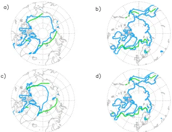
Fig. 10.Sea-ice edge (15 % sea-ice concentration limit) location in the HadGEM2-ES (blue line) and the MIROC-ESM (green line). The upper panels show the(a)minimum and(b) maximum sea-ice limit in the pre-industrial climate. The lower panels show the (c)minimum and(d)maximum sea-ice limit in the mid-Holocene climate. The change in the sea-ice edge location from MH to PI is larger for the minimum ice extent, especially for the HadGEM2-ES model.
shown in Fig. 10a and b, respectively. In the PI climate, the HadGEM2-ES model simulates slightly thicker ice than the MIROC-ESM. The HadGEM2-ES (Fig. 11a) simulates the thickest ice in the Canadian Archipelago in the month of min-imum sea-ice extent. The MIROC-ESM (Fig. 11b) simulates the thickest ice in the central Arctic Ocean. The HadGEM2-ES also simulates a stronger seasonal variation, and larger variability in the simulated sea-ice extent than the MIROC-ESM (Fig. 9a).
4.3.2 Response to the MH forcing
The MIROC-ESM and HadGEM2-ES both show a similar sensitivity of the sea-ice extent in the future RCP-scenarios. They both reach nearly ice-free conditions (minimum sea-ice extent smaller than 106km2) at around 2050 AD, regard-less of RCP scenario. The MIROC-ESM reaches this state slightly faster than the HadGEM2-ESM for all three RCP-scenarios (see Fig. 2 in Wang and Overland, 2012).
The 2×CO2 equilibrium climate sensitivity of the two
models is 4.6 K (HadGEM2-ES) and 4.7 K (MIROC-ESM) (Andrews et al., 2012). The 2×CO2 equilibrium climate
sensitivity is the increase in global surface-temperature in response to an instantaneous doubling of CO2, after the
model has equilibrated. The climate sensitivity estimated of Andrews et al. (2012) show that the HadGEM2-ES model is more sensitive (1.6 K Wm−2) than the MIROC-ESM (1.1 K Wm−2). The similar 2×CO2 equilibrium re-sponse is explained by the fact that a CO2 increase yields
Fig. 11.Sea-ice thickness in the pre-industrial simulation for the minimum ice extent for(a)the HadGEM2-ES and(b)the MRIOC-ESM. Only ice thicker than 15 cm is included in the figure.
a stronger climate forcing in the MIROC-ESM than the HadGEM2-ES.
When exposed to the MH insolation forcing, the MIROC-ESM simulates one of the weakest sea-ice responses in the PMIP3 ensemble and the HadGEM2-ES one of the strongest (see Table 1). In HadGEM2-ES, the Arctic sea-ice extent de-creases throughout the year in the MH climate (see Fig. 9b). The minimum sea-ice extent experiences the the strongest reduction in the eastern Arctic (see the blue line in Fig. 10a and c). In MIROC-ESM the changes are generally small (see Fig. 9b), with a slight increase in the maximum sea-ice ex-tent, mainly in the Labrador sea (see the green line in Fig. 10b and d).
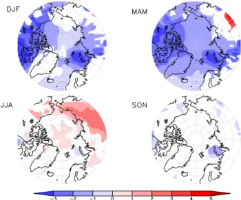
HadGEM2-ES experiences a warming in the Arctic throughout the year, with the most pronounced warming oc-curring in autumn (SON) and winter (DJF) (Fig. 12). The MIROC-ESM, on the other hand, simulates a cooling in the MH winter and spring (MAM), with a weak warming in the summer season (JJA). In autumn, there are essentially no sig-nificant changes in the surface air temperature north of 60◦N (Fig. 13). In the light of the land-based proxy temperature reconstructions, analysed by Zhang et al. (2010), it can be concluded that the year around warming in the HadGEM2-ES model is more consistent with data.
4.3.3 Cloud impact on the insolation forcing
Given the different responses of the HadGEM2-ES and MIROC-ESM model it is relevant to try to identify the un-derlying mechanisms. One possibility is that this difference is related to model differences in clouds and albedo. To ex-amine this issue, we consider the shortwave cloud forcing at surfaceCSW, which is defined as
CSW=FSWall −FSWclr, (6)
where FSW is the downward shortwave radiation at the
Fig. 12.Change in surface temperature (◦C) north of 60◦N from mid-Holocene to pre-industrial in the HadGEM2-ES, for winter, spring, summer and autumn. Only changes statistically significant at a 95 % confidence level are shown. A clear warming can be seen for all seasons in the mid-Holocene climate.
represents the reduction of the surface shortwave radiation due to clouds, and is generally negative.
Clouds have a stronger effect on summer surface short-wave radiation in the MIROC-ESM than in the HadGEM2-ES in both the PI and MH simulations (Fig. 14). Thus, the effect of the increased insolation in the MH is more strongly muted by clouds in the MIROC-ESM, which should con-tribute to the weaker sea-ice extent reduction and north-ern high-latitude warming observed in that model; see e.g. Fig. 15.
Both models simulate a stronger cloud effect on summer surface shortwave radiation in the MH than in the PI simula-tion. This difference is consistent with the combined effect of a larger cloud fraction in the MH than in the PI (not shown) and higher incoming shortwave radiation at the top of the atmosphere due to orbital forcing. At the top of the atmo-sphere, these competing effects combine to higher absorbed shortwave radiation (i.e. incoming minus outgoing shortwave radiation at the top of the atmosphere) as shown in Fig. 15.
5 Discussion
The new generation climate models used in CMIP5 and PMIP3 simulate a smaller and thinner Arctic sea ice in bet-ter agreement with observations (Stroeve et al., 2012; Bj¨ork et al., 2013). This can partly explain the higher sensitivity of the ice cover to the increased MH summer insolation in these models as compared to the previous generation models in PMIP2.
Fig. 13.Change in surface temperature (◦C) north of 60◦N from mid-Holocene to pre-industrial in the MIROC-ESM, for winter, spring, summer and autumn. Only changes statistically significant at a 95 % confidence level are shown. The strongest temperature responses occur in winter and spring, where the mid-Holocene cli-mate is colder than the pre-industrial.
The thinner ice in the PMIP3 models will absorb more so-lar radiation than the thicker ice in the PMIP2 models. In one-dimensional thermodynamic sea-ice models, this effect is known to play a critical role for transitions between states with perennial, seasonal, and no sea ice (e.g. Abbot et al., 2011; Moon and Wettlaufer, 2012; Bj¨ork et al., 2013). For instance in the one-dimensional model study of Bj¨ork et al. (2013), the sea-ice cover reaches a transition from perennial to seasonal ice when the annual-mean sea-ice thickness drops below about 2 m. A generally thinner sea-ice cover may also contribute to explain the increased seasonality of the sea ice in the PMIP3 models: as the sea-ice thickness is reduced, the ice generally becomes more variable (Holland et al., 2008; Bitz and Roe, 2003).
There are some noteworthy differences in the response of the Arctic sea-ice cover to increased CO2forcing and the
or-bital forcing associated with the MH. Essentially all CMIP3 and CMIP5 models simulate decreased winter maximum and summer minimum sea-ice extent in response to an increased CO2 forcing (Eisenman et al., 2011; Stroeve et al., 2012).
Fig. 14.Summer (JJA) cloud radiative shortwave forcing at the sur-face (W m−2). Left panel (aandc) show the pre-industrial condi-tions, right panel (bandd) show the mid-Holocene conditions. Up-per row shows results from the HadGEM2-ES (aandb) and lower row shows results from the MIROC-ESM (candd). Note that the clouds have a stronger cooling effect at the surface in the MIROC-ESM model.
the effective climate forcing that arises due to the changes in incoming shortwave radiation at the top of the atmosphere is strongly regulated by the cloud cover and the surface albedo in the background climate. On the other hand, the radiative forcing due to increases of CO2 is likely to be less
sen-sitive to the background climate; the vertical temperature structure and cloud distribution are influencing factors (e.g., Pierrehumbert, 2010; Andrews et al., 2012; Solomon et al., 2007, chapter 2.2). Against this background, it is not sur-prising that the climate models’ Arctic sea-ice responses are more consistent for a doubling of CO2 forcing than for the
orbitally induced forcing between MH and PI. It should also be noted that the changes in Arctic sea-ice cover between the mid-Holocene and the pre-industrial era shown in Fig. 5 are smaller for many of the models than the observed change in ice cover over the last 30 yr. Thus, it cannot be ruled out that internal model variability may obscure the response to the orbital forcing in some of the models with a weak response (Goosse et al., 2007).
One result that is reasonably robust among the model re-sponses to the orbitally induced forcing is the correlation be-tween the annual-mean change in the Arctic sea-ice extent and the summer surface air temperature increase north of 60◦N (Fig. 6).
As has been suggested by Goosse et al. (2007) one may obtain stronger response in the Arctic and smaller and thinner sea-ice covers if one considers the earlier part of the Holocene (around 9 to 8 ka BP) rather than the mid-Holocene. This may be a better period to use for investigation
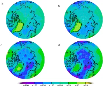
Fig. 15.Change in the top of the atmosphere absorbed solar ra-diation (W m−2) from MH to PI, for(a)HadGEM2-ES and(b) MIROC-ESM. Only changes statistically significant at a 95 % con-fidence level are shown. The increase in mid-Holocene shortwave absorption is stronger in HadGEM2-ES than MIROC-ESM.
of the model response to the changes in solar insolation, since the orbital insolation forcing was stronger then. However, as pointed out by Renssen et al. (2005) remnant ice sheets may have had a cooling effect on the Arctic climate in this early part of the Holocene, and possibly also in later stages. Note that in the PMIP mid-Holocene protocol there are no remnant ice sheets.
6 Conclusions
The main findings of this study are:
– The models (PMIP2 + PMIP3) all yield a smaller and thinner Arctic summer sea-ice cover in the MH than in the PI control climate. Differences in the winter sea-ice extent and thickness are smaller in amplitude with an approximately equal distribution of models with larger/smaller sea-ice extent in MH than in PI.
– The new generation climate models (PMIP3) simulate thinner and smaller extents for the Arctic sea ice than the previous generation climate models (PMIP2), both in the pre-industrial and the mid-Holocene simulations.
– The sea-ice thickness response of the models north of 80◦N follows roughly the behaviour predicted by the model of Thorndike (1992) with an assumed increase in sea-ice melt of 0.2 m per year; see Fig. 3.
– In the models’ simulated changes between the PI and the MH, there is a strong correlation between the in-crease of summer surface air temperature north of 60◦N and the annual mean decrease of the sea-ice extent; see Fig. 6.
– Models that respond similarly to CO2forcing may
simulate the recent observed decline in sea ice well, and they respond similarly to future CO2forcing.
How-ever, the two models’ responses to the change in so-lar forcing are significantly different: the HadGEM2-ES is more sensitive and experiences a more pronounced warming and stronger decrease in the minimum sea-ice extent than the MIROC-ESM. One plausible explana-tion for the difference in sensitivity is that the MIROC has higher cloud fractions in the summer Arctic, which acts to mute the effects of the solar forcing.
– In the PMIP ensemble, there are models that simulate large areas of open water east of Greenland for the mid-Holocene. These areas could provide the fetch for the surface waves needed to form the beach ridges in north-eastern Greenland found in sea-ice proxy data (Funder et al., 2011) and Jakobsson et al. (2010).
Acknowledgements. The Bert Bolin Centre for Climate Research
at Stockholm University, funded by the Swedish research councils VR and FORMAS, provided founding for this work. We thank Arne Johansson, referee P. Brohan and one anonymous referee for comments on the manuscript. We acknowledge the World Climate Research Programme’s Working Group on Coupled Modelling, which is responsible for CMIP, and we thank the climate modeling groups (listed in Table 1 of this paper) for producing and making available their model output. For CMIP the US Department of Energy’s Program for Climate Model Diagnosis and Intercom-parison provides coordinating support and led development of software infrastructure in partnership with the Global Organization for Earth System Science Portals. We acknowledge the interna-tional modelling groups for providing their data for analysis, the Laboratoire des Sciences du Climat et de l’Environnement (LSCE) for collecting and archiving the model data. The PMIP 2 Data Archive is supported by CEA, CNRS and the Programme National d’Etude de la Dynamique du Climat (PNEDC). The analyses were performed using version 01-20-2010 of the database. More information is available on http://pmip2.lsce.ipsl.fr/.
Edited by: M. Crucifix
References
Abbot, D. S., Silber, M., and Pierrehumbert, R. T.: Bifurcations leading to summer Arctic sea-ice loss, J. Geophys. Res., 116, D19120, doi:10.1029/2011JD015653, 2011.
Andrews, T., Greory, J. M., Webb, M. J., and Taylor, K. E.: Forcing, feedbacks and climate sensitivity in CMIP5 coupled atmosphere-ocean climate models, Geophys. Res. Lett., 39, L09712, doi:10.1029/2012GL051607, 2012.
Backman, J., Moran, K., McInroy, D. B., and Mayer, L. A.: Ex-pedition 302 scientist: Proceedings of IODP, 302, Integrated Ocean Drilling Program Management, Internation, Inc. Eding-burgh, 2006.
Berger, A. L.: Long-term variations of daily insolation and Quater-nary climatic changes, J. Atmos. Sci., 35, 2362–2367, 1978.
Bitz, C. M. and Roe, G. H.: A mechanism for the high rate of sea-ice thinning in the Arctic Ocean, J. Climate, 17, 3623–3632, 2003. Bj¨ork, G., Stranne, C., and Boren¨as, K.: The sensitivity of the
Arctic Ocean sea-ice thickness and its dependence on the surfrace albedo parameterization, J. Climate, 26, 1355–1370, doi:10.1175/JCLI-D-12-00085.1, 2013.
Braconnot, P., Otto-Bliesner, B., Harrison, S., Joussaume, S., Pe-terchmitt, J.-Y., Abe-Ouchi, A., Crucifix, M., Driesschaert, E., Fichefet, Th., Hewitt, C. D., Kageyama, M., Kitoh, A., Laˆın´e, A., Loutre, M.-F., Marti, O., Merkel, U., Ramstein, G., Valdes, P., Weber, S. L., Yu, Y., and Zhao, Y.: Results of PMIP2 coupled simulations of the Mid-Holocene and Last Glacial Maximum – Part 1: experiments and large-scale features, Clim. Past, 3, 261– 277, doi:10.5194/cp-3-261-2007, 2007a.
Braconnot, P., Otto-Bliesner, B., Harrison, S., Joussaume, S., Pe-terchmitt, J.-Y., Abe-Ouchi, A., Crucifix, M., Driesschaert, E., Fichefet, Th., Hewitt, C. D., Kageyama, M., Kitoh, A., Loutre, M.-F., Marti, O., Merkel, U., Ramstein, G., Valdes, P., Weber, L., Yu, Y., and Zhao, Y.: Results of PMIP2 coupled simula-tions of the Mid-Holocene and Last Glacial Maximum – Part 2: feedbacks with emphasis on the location of the ITCZ and mid- and high latitudes heat budget, Clim. Past, 3, 279–296, doi:10.5194/cp-3-279-2007, 2007b.
Braconnot, P., Harrison, S. P., Otto-Bliesner, B., Abe-Ouchi, A., Jungcalus, J., and Peterschmitt, J.-Y.: The Paleoclimate Mod-elling Intercomparison Project contribution to CMIP5, CLIVAR Exchanges No. 56, 16, 15–19, 2011.
Cavalieri, D., Parkinson, C., Gloersen, P., and Zwally, H. J.: sea-ice concentration from Nimbus-7 SMMR and DMSP SSM/I-SSMIS Passive Microwave Data, [1979–2008], Boulder, Colorado USA: National Snow and Ice Data Centre. Digital Media, 2008. de Vernal, A., Hillaire-Marcel, C., Solinac, S., and Radi, T.:
Recon-structing sea-ice conditions in the Arctic and Sub-Arctic prior to human observations, edited by: Weaver, E., Arctic sea-ice De-cline: Observations, Projections, Mechanisms, and Implications, AGU Monograph Series 180, 27–45, 2008.
Donohoe, A. and Battisti, D. S.: Atmospheric and Surface Contri-butions to Planetary Albedo, J. Climate, 24, 4402–4418, 2011. Eisenman, I., Schneider, T., Battisti, D. S., and Bitz, C. M.:
Consis-tent Changes in the sea-ice Seasonal Cycle in Response to Global Warming, J. Climate, 24, 5325–5335, 2011.
Funder, S., Goosse, H., Jepsen, H., Kaas, E., Kjær, K. H., Kors-gaard, N. J., Larsen, N. K., Linderson, H., Lysaa, A., M¨oller, P., Olsen, J., and Willerslev, E.,: A 10 000-year record of Arctic Ocean sea-ice variability – View from the beach, Science, 333, 747–750, 2011.
Goosse, H., Driesschaert, E., Fichefet, T., and Loutre, M.-F.: In-formation on the early Holocene climate constrains the summer sea ice projections for the 21st century, Clim. Past, 3, 683–692, doi:10.5194/cp-3-683-2007, 2007.
Hartman, D. L.: Global Physical Climatology, Academic Press, Cal-ifornia, 1994.
Holland, M. M., Serreze, M. C., and Stroeve, J.: The sea-ice mass budget of the Arctic and its future change as simu-lated by coupled climate models, Clim. Dynam., 34, 185–200, doi:10.1007/s00382-008-0493-4, 2008.
Jakobsson, M., Long, A., Ing´olfsson, ´O., Kjær, K. H., and Spielha-gen, R. F.: New insights on Arctic Quaternary climate variabil-ity from paleo-records and numerical modelling, Quaternary Sci. Rev., 29, 3349–3358, 2010.
Kwok, R. and Rothrock, D. A.: Decline in Arctic sea-ice thickness from submarine and ICESat records: 1958–2008, Geophys. Res. Lett., 36, L15501, doi:10.1029/2009GL039035, 2009.
Levitus, S., Boyer, T. P., Conkright, M. E., O’Brien, T., Antonov, J., Stephens, C., Stathoplos, L., Johnson, D., and Gelfeld, R.: NOAA Atlas NESDIS 18, World Ocean Database 1998: Volume 1: Introduction, 1998.
Moon, W. and Wettlaufer, J. S.: On the existence of stable season-ally varying Arctic sea-ice in simple models. J. Geophys. Res., 117, C07007, doi:10.1029/2012JC008006, 2012.
Notz, D. and Marotzke, J.: Observations reveal external driver for Arctic sea-ice retreat, Geophys. Res. Lett., 39, L08502, doi:10.1029/2012GL051094, 2012.
Otto-Bliesner, B. L., Brady, E. C., Clauzet, G., Tomas, R., Levis, S., and Kothavala, Z.: Last Glacial Maximum and Holocene climate in CCSM3, J. Climate, 19, 2526–2544, 2006.
Pierrehumbert, R. T.: Principles of Planetary Climate, Cambridge Univ. Press, NY, 2010.
Polyak, L., Alley, R. B., Andrews, J. T., Bringham-Grette, J., Cronin, T. M., Darby, D. A., Dyke, A. S., Fritzpatrick, J. J., Fun-der, S., Holland, M., Jennings, A. E., Miller, G. H., O’Regan, M., Savelle, J., Serreze, M., St.John, K., White, J. W. C., and Wolff, E.: History of sea-ice in the Arctic, Quaternary Sci. Rev., 29, 1757–1778, 2010.
Renssen, H., Goosse, H., Fichefet, T., Brovkin, V., Driesschaert, E., and Wolk, F.: Simulating the Holocene climate evolution at northern high latitudes using a coupled atmosphere-sea-ice-ocean-vegetation model, Clim. Dynam., 24, 23–43, 2005. Renssen, H., Sepp¨a, H., Hein, O., Roche, D. M., Goosse, H.,
and Fichefet, T.: The spatial and temporal complexity of the Holocene thermal maximum, Nat. Geosci., 2, 411–414, doi:10.1038/NGEO513, 2009.
Rothrock, D. A., Zhang, J., and Yu, Y.: The Arctic sea-ice thickness anomaly of the 1990s: A consistent view from observations and models, J. Geophys. Res., 1008, 3083, doi:10.1029/2001JC001208, 2003.
Serreze, M. C., Holland, M. M., and Stroeve, J.: Perspectives on the Arctic’s shrinking sea-ice cover, Science, 3115, 1533–1536, 2007.
Solomon, S., Qin, D., Manning, M., Chen, Z., Marquis, M., Averyt, K. B., Tignor, M., and Miller, H. L. (Eds.): Climate Change 2007, The Physical Science Basis, Contribution of Working Group 1 to the Fourth Assessment Report of the Intergovernmental Panel on Climate Change, 2007.
Stroeve, J., Kattsov, V., Barrett, A., Serreze, M., Pavlova, T., Hol-land, M., and Meier, W. N.: Trends in Arctic sea-ice extent from CMIP5, CMIP3 and observations, Geophys. Res. Lett., 39, L16502, doi:10/1029/2012GL052676, 2012.
Thorndike, A. S.: A toy model linking atmospheric thermal radia-tion and sea-ice growth, J. Geophys. Res., 97, 9401–9410, 1992. Wallace, C. J. and Osborn, T. J.: Recent and future modulation of
the annual cycle, Clim. Res., 22, 1–11, 2002.
Wang, M. and Overland, J. E.: A sea-ice free summer Arctic within 30 years: An update from CMIP5 models, Geophys. Res. Lett., 39, L18501, doi:10.1029/2012GL052868, 2012.
Winton, M.: Do Climate Models Underestimate the Sensitivity of Northern Hemisphere Sea Ice Cover?, J. Climate, 24, 3924– 3934, 2011.