www.clim-past.net/5/803/2009/
© Author(s) 2009. This work is distributed under the Creative Commons Attribution 3.0 License.
of the Past
On the importance of paleoclimate modelling for improving
predictions of future climate change
J. C. Hargreaves and J. D. Annan
Global Change Projection Research Program, Research Institute for Global Change, JAMSTEC, 3173-25 Showa-machi, Kanazawa-ku, Yokohama City, Kanagawa, 236-0001, Japan
Received: 21 July 2009 – Published in Clim. Past Discuss.: 29 July 2009
Revised: 23 October 2009 – Accepted: 1 December 2009 – Published: 21 December 2009
Abstract. We use an ensemble of runs from the MIROC3.2 AGCM with slab-ocean to explore the extent to which mid-Holocene simulations are relevant to predictions of future cli-mate change. The results are compared with similar analy-ses for the Last Glacial Maximum (LGM) and pre-industrial control climate. We suggest that the paleoclimate epochs can provide some independent validation of the models that is also relevant for future predictions. Considering the paleo-climate epochs, we find that the stronger global forcing and hence larger climate change at the LGM makes this likely to be the more powerful one for estimating the large-scale changes that are anticipated due to anthropogenic forcing. The phenomena in the mid-Holocene simulations which are most strongly correlated with future changes (i.e., the mid to high northern latitude land temperature and monsoon pre-cipitation) do, however, coincide with areas where the LGM results are not correlated with future changes, and these are also areas where the paleodata indicate significant climate changes have occurred. Thus, these regions and phenomena for the mid-Holocene may be useful for model improvement and validation.
1 Introduction
Model predictions of long term climate change cannot be val-idated through repeated forecast/analysis cycles in the same manner as weather forecasts, as the necessary time scale is too long. Models are routinely evaluated in terms of how well they represent current climate, although this only ap-pears to provide rather limited evidence for their future per-formance (Whetton et al., 2007; Abe et al., 2009). Re-searchers have, therefore, been motivated to look for times
Correspondence to:J. C. Hargreaves
in the past when the climate was rather different to today, because a model that does a good job of modelling paleocli-mates may reasonably be considered preferable to one that does not. However, this hypothesis is so far largely untested. Similar processes do not necessarily govern all past and fu-ture climate changes, so it is arguable that what we really should seek are those climate changes in the past that are in some way analogous to or informative regarding the future changes we expect to see.
As observational evidence tends to become more sparse and uncertain at more distant times, much effort has been focussed on more recent paleo-climates such as the mid-Holocene (6 ka BP) and Last Glacial Maximum (LGM, 21 ka BP). Model simulations of these epochs have formed the centrepiece of Paleoclimate Modelling Inter-comparison Projects PMIP and PMIP2 (Joussaume et al., 1999; Bracon-not et al., 2007a). However, there is relatively little research directly addressing the extent to which these paleoclimate epochs are informative or the processes governing the cli-mate changes analogous to those effecting future change. For example, one might question how essential it is to ac-curately simulate the response and climate feedbacks due to the huge ice sheets present over large parts of the Northern Hemisphere at the LGM, since for the modern climate and in coming decades, we expect at most small changes in the amount of terrestrial ice. However, at the LGM, there was also a significant decrease in the the forcing from greenhouse gases (primarily CO2) compared to present day levels, and
we may expect that the response to this forcing involves sim-ilar processes to those relevant to future change.
limitations of the model. They found a reasonably strong cor-relation between the climate changes for the LGM and dou-bled CO2, especially away from the large Northern
Hemi-sphere ice sheets. Using a simpler atmospheric model (but a three-dimensional ocean), Schneider von Deimling et al. (2006) obtained broadly comparable results. However, Cru-cifix (2006) examined results from 4 distinct AOGCMs and found no evidence of a relationship between the climate changes seen at the LGM and 2×CO2states, although with
such a small ensemble, statistical significance would be hard to achieve. Thus, the results obtained here must be consid-ered in the context of the single model that underlies the experiments. Since multi-model experiments are obviously outside our capabilities, we hope that our results will encour-age other groups to attempt similar investigations.
In this paper we explore the climate changes for the mid-Holocene to see to what extent modelling that epoch may help improve forecasts of future climate, and compare our results to similar analysis of LGM simulations. Although paleoclimate studies are gaining in popularity, most compar-ison with data for GCMs is made against the present day climatology. Therefore, to further set this work in context we also compare the results to similar analyses for the pre-industrial control simulation. The mid-Holocene might ap-pear at first to be a rather weak analogue for future climate change since at this epoch there are no large changes in the net forcing or greenhouse gas levels. Moreover, the over-all climate changes at the mid-Holocene are rather different in character compared to those expected to occur in the fu-ture (Mitchell, 1990). Thus, we do not expect the climate changes to be a close analogue in the sense of being di-rectly applicable to future projections. Rather, we are look-ing for climate phenomena that respond to the same uncer-tain inputs, so that, as Mitchell (1990) proposes, analysis of paleoclimate changes might be useful for the estimation of model parameters that also control future changes. Paleo-data from the mid-Holocene do indicate some significant changes which may be relevant to future climate change. The most prominent example is the evidence that the monsoon re-gions extended further northward than today, a result shown most dramatically by evidence for greening of parts of the present day Sahara desert (Jolly et al., 1998). Current pre-dictions for the future changes of the monsoon under global change are highly uncertain, with disagreement in the mod-els over the sign of the precipitation change (e.g. Fig. 10.9, Solomon et al., 2007). Therefore in this paper we analyse monsoon changes as well as zonal and global changes.
2 Boundary conditions for mid-Holocene and LGM climate simulations
The forcing for the mid-Holocene in the PMIP2 proto-col (Braconnot et al., 2007a) consists of a small change to the CH4 concentration relative to the pre-industrial level (from
760 ppm to 650 ppm) and a change in the orbital forcing cal-culated from Berger (1978). The change to the orbital forc-ing affects the seasonal cycle and also changes the lengths of the seasons by up to 5 days (Joussaume and Braconnot, 1997). The use of the classical calendar for both experi-ments results in a mismatch between monthly results when compared to a true solar calendar. However, the analysis dis-cusssed in this paper pertains to assessing correlations be-tween variables over the ensemble, and we expect the effect of this calendar inaccuracy on our results to be small since it affects all ensemble members equally. The PMIP2 protocol for the LGM consists of a significant decrease in the levels of greenhouse gases compared to the modern climate, the in-clusion of fixed massive ice sheets over the Northern Hemi-sphere and a small change in the orbital forcing (see Bracon-not et al., 2007a for details). We also performed the PMIP2 pre-industrial control (CTRL) and a future climate experi-ment which has an increased carbon dioxide concentration but is otherwise identical to the pre-industrial.
3 Method
For our experiments we use a 36 member ensemble of runs of the MIROC3.2 AGCM with slab ocean, at T21 resolu-tion. The ensemble generation method closely follows An-nan et al. (2005), in which an ensemble Kalman filter was used for multivariate parameter estimation by tuning the model to various fields of modern climatological data, pro-ducing a 40 member ensemble. However, in this experi-ment we only allowed 13 model parameters to vary (selecting those which had been found to most strongly influence model results). We use a slab ocean model to reduce the equilibra-tion time of the model, as is usual for such perturbed param-eter ensemble experiments (e.g. Murphy et al., 2004). This requires the calculation of implied heat fluxes at each grid box (the so-called Q-flux field) to mimic the lateral trans-port of heat (Russell et al., 1985). Although in principle this flux field should integrate to zero for an equilibrium state, if no particular care is taken, the Q-flux field may have a large nonzero integral, indicating that the model is far from radiative balance under modern conditions. We found that in our previous work, there was a substantial radiative im-balance of around 10Wm−2both for the ensemble members, and also for the unperturbed model when run at T21 resolu-tion. Therefore, in this experiment, we imposed an additional constraint on the global and annual average of the Q-flux to reduce the radiative imbalance to around 2Wm−2, similar to or lower than the results of Collins et al. (2006). Further de-tails of the ensemble are described in Yokohata et al. (2009). All the runs are at least 40 years long, with the last 20 years averaged to provide the results. The imposition of the Q-flux constraint resulted in an increase in the climate sensitivity of the ensemble, to 7.0±3.7◦C (2 standard deviations). For the
with higher control temperature and high sensitivity became unstable once the global mean surface temperature exceeded
∼296 K. According to the IPCC AR4, climate sensitivity is likely to lie in the range 2–4.5◦C (IPCC 2007: summary for Policymakers, Solomon et al., 2007). In this experiment we are, therefore, exploring the climate behaviour for the un-likely higher values of climate sensitivity. Given the interest in the possible consequences of such high sensitivities, in or-der to obtain a stable ensemble which could reasonably be used for analysis, we performed another experiment using
√
2 times pre-industrial CO2levels which reduces the
librium warming by 50% (for those models which do equi-librate). Apart from one ensemble member which crashed early on, and is also pathological for the LGM climate, all the other 39 ensemble members remained stable for a long run (>150 years) with this forcing. Here we use the results
from the larger √2×CO2 ensemble but double the climate
changes to ease comprehension of the values in the context of other literature, and refer hereafter to the result as 2×CO2.
For the LGM, one other ensemble member produced a state about 6◦C colder than the ensemble mean so this is consid-ered to not represent a reasonable LGM and is excluded from the ensemble. Such abnormal cooling can be produced by a physically unrealistic cloud or sea-ice feedback and is a well-known limitation of slab ocean models. The final 36 member ensemble is produced by further excluding two more ensem-ble members which produced similarly very cold states for a LGMGHG simulation (pre-industrial conditions with LGM greenhouse gases), that is not discussed in this paper, but is the subject of other analyses currently underway.
The underlying basis for our work is the expectation that our ensemble of models with varying parameters rep-resents at least a large subset of our uncertainties concern-ing the physical processes controllconcern-ing past and future cli-mate change. We note that in support of this claim, the fu-ture projections for monsoon changes in this model ensem-ble (discussed in more detail later) include both increases and decreases in precipitation, similar to that exhibited by the IPCC ensemble of opportunity mentioned above. The first-order relationship between past and future data can be expressed as their covariances, which describes how the un-certainties in the future changes are related to unun-certainties in past changes. If the covariance is low, then information about the past will not influence future predictions, but if the covariance is high, then this implies that information about the past will propagate into predictions. Therefore, we now explore our ensemble results to investigate where such rela-tionships may exist. This approach is similar to the general principles underlying Observing System Simulation Exper-iments (Arnold Jr. and Dey, 1986), by which the value of observational data for prediction systems can be considered. However in this work here do not quantify the likely bene-fits, which also depends on the precision of the observational evidence that might be available.
Another important issue is that of the model inadequacy, that is the fact that the model cannot simulate reality per-fectly foranyset of parameter values. Moreover, different model ensembles may well exhibit somewhat different rela-tionships between past and future climate, depending on their structure and parameterisations. The relationship is a prop-erty of the model and experimental details, rather than the climate system itself (which has one past and future trajec-tory). Therefore, while the existence of relationship between past and future climate (within a model ensemble) is a pre-requisite in order for paleoclimate tuning to affect the future predictions, this may not be sufficient by itself to assure that the tuning will actually lead to improvements. We cannot address this question within this paper, but hope that the is-sues relating to this question can be further explored using ensembles of different models (e.g. Yokohata et al., 2009).
4 Results
4.1 Analysis of annual averages on the global scale The difference between the control and mid-Holocene an-nually and globally averaged global 2 m temperatures (here-after, T2) is rather small (0.3±0.2◦C at 1 standard deviation),
reflecting the small change in the mean climate forcing. The correlation coefficient between the temperature change and climate sensivity is less than 0.1. These results are not unex-pected given the net forcing change is a small proportion of the seasonal and regional forcing. For the LGM simulations, MIROC shows a fairly strong correlation coefficient of 0.74 between the change in T2 from control to LGM, and climate sensitivity, consistent with but slightly higher than in previ-ous work (Annan et al., 2005). These results are illustrated in Fig. 1. For reference, the level of statistical significance at 1% for a sample size of 36, assuming independent samples, is 0.42 according to Student’s t-test. While in our results we have used the 1% significance level as a guide to the signif-icance of our results, it should be noted that in this work we have considered over 1000 different correlation coefficients, meaning that a number of false positives are to be expected in the results. A larger model ensemble, which is not at present computationally feasible, would improve the statistical con-fidence of our results.
For clarity and brevity, the three experiment-control differ-ences for the 2×CO2, LGM, and mid-Holocene experiments
are abbreviated to D2×CO2, DLGM and D6ka, respectively.
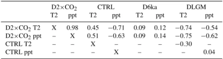
Table 1 shows, for T2 and precipitation, the correlation co-efficients between D2×CO2and the other experiments. For
T2, the control is significantly correlated with D2×CO2, but
Climate Sensitivity (oC)
T2 (
oC)
correlation coeffs red: 0.74
blue: 0.60
magenta: 0.09
red: (CTRL-LGM) low QFLUX ensemble vs. Climate sensitivity
blue: (CTRL-LGM) 120 member ensemble vs. Climate sensitivity
magenta: (6ka-CTRL) low QFLUX ensemble vs. Climate sensitivity
Fig. 1. Correlation between the temperature changes for 2×CO2
and the two experiments, LGM and mid-Holocene. The blue dots show the results from previous work on the LGM, indicating that the results for the new low Q-flux ensemble are consistent, although of slightly higher sensitivity. The contrast between the strong signal for the LGM and very small global change for the mid-Holocene is clear.
global D2×CO2 temperature change using the DLGM and
control temperatures (singly or jointly) as predictors. The control value alone explains 21% of the total variance, with the LGM explaining 55% and both control and LGM to-gether combining to explain 61%.
For D2×CO2, there is an extremely high correlation
be-tween temperature and precipitation, so it is not surpris-ing to also see significant correlation coefficients for the correlation of control and DLGM temperatures with pre-cipitation for D2×CO2. Although the correlations
indi-cate that a higher control temperature leads to increased cli-mate sensitivity, and increased global precipitation change for D2×CO2, higher control precipitation leads to a smaller
precipitation change for increased CO2. In contrast, for the
LGM, the global precipitation changes are negative, and the larger the change in precipitation the greater the precipita-tion change for increased CO2. The negligible correlation
between the control and DLGM precipitation suggests that these aspects of the LGM and control climates may be de-termined by (and therefore useful for constraining) different, independent processes in the model, and thus the informa-tion from both epochs may combine effectively. A similar regression analysis to the previous paragraph reveals that the control and DLGM results each explain almost 40% of the total variance of the D2×CO2precipitation change, and in
combination they explain 75% of the total variance. Again, the mid-Holocene makes a negligible contribution.
Table 1.Correlation between the global temperature and
precipita-tion for the various experiments.
D2×CO2 CTRL D6ka DLGM
T2 ppt T2 ppt T2 ppt T2 ppt
D2×CO2T2 X 0.98 0.45 −0.71 0.09 0.12 −0.74 −0.54
D2×CO2ppt – X 0.51 −0.63 0.09 0.14 −0.75 −0.62
CTRL T2 – – X – – – −0.30 –
CTRL ppt – – – X – – – 0.04
4.2 Analysis of annual averages on the zonal scale One of the potential difficulties of using paleo-climate data to validate climate models is the mismatch in spatial scales between the GCMs, which are most reliable at the largest scales, and less so at smaller scales, versus paleoclimate data, which is generally highly local in nature. So, while the global calculations presented above indicate that there are links be-tween the processes effecting climate changes at the LGM and 2×CO2climates, they do not shed any light on which
regions may be effectively used to validate and improve the modelled predictions of future climate change. In addition, the changes in climate at the mid-Holocene, being caused by changes in the patterns of seasonal forcing, are expected to be far greater on zonal to regional scales than at the global average. The albedo forcing due to ice sheets at the LGM is also strongly linked to latitude. Thus we consider the relationship in the ensemble between the zonally averaged variables for D2×CO2, DLGM, D6ka, CTRL and the global
scale changes for 2×CO2. The mid-Holocene results
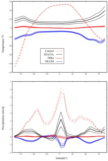
pro-vide a very small contribution, explaining less than 1% of the variance. The zonally averaged annual average temper-atures for CTRL, D2×CO2, D6ka and DLGM are shown in
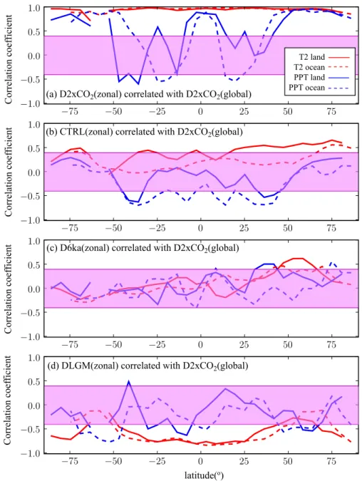
Fig. 2. The heavier lines are the ensemble mean, whereas the lighter weight lines show the one standard deviation widths of the ensembles. The results from the correlation analysis are shown in Fig. 3. The red lines show the correlation of zonal and global temperature, and the blue show the correla-tion of zonal and global precipitacorrela-tion. As paleoclimate data for land and ocean is often analysed and synthesised indepen-dently, the correlation analysis is done for the land and ocean separately (solid and dashed lines, respectively). As shown in Fig. 3a, for D2×CO2 the temperature is strongly
Control D2xCO2 D6ka DLGM
latitude(o)
Precipitation mm/dy
T
empertaure
oC
Fig. 2.Top: annually averaged temperature for the control climate,
and the differences between the control and the simulated climates. The thinner lines show the 1 standard deviation ranges of the en-semble. Bottom: the same as the top plot, but for precipitation.
For D6ka (Fig. 3c) the correlation coefficients are mostly below the level of the noise, except for part of the North-ern Hemisphere where the correlation is reasonably strong over the land in particular. Interestingly, this is the same lat-itude range for which the correlation coefficient for DLGM (Fig. 3d) temperature is rather weak, due to the existance of the large ice sheets (which was previously discussed in Har-greaves et al., 2007). In addition, for DLGM, as we noted in previous work (Hargreaves et al., 2007), although the corre-lation for temperature is generally very strong, small biases in the control sea-ice extent may strongly influence the tem-perature in the sea-ice region for increasing CO2, leading to
no significant correlation for temperature in the sea-ice re-gions for DLGM. The situation for precipitation is, however, reversed with the correlation coefficient being rather strong for DLGM over the ocean from 40–70◦S.
From these results it would appear that the best data to use to improve the model predictions would be the temperatures in the tropics and very high latitudes along with
precipita-tion in the southern ocean at the LGM, the mid-to-high lat-itude temperatures for the Northern Hemisphere at the mid-Holocene and the whole of the Northern Hemisphere tem-peratures and tropical precipitation for the pre-industrial cli-mate. Given the very high correlation between the global temperature and precipitation for D2×CO2, the correlations
for zonal temperature with global precipitation (not shown) look almost identical to the red lines in Fig. 3, and indi-cates that improving the temperature should also result in improved precipitation.
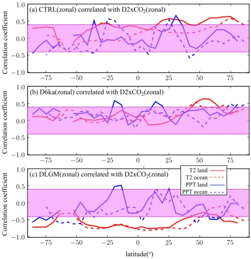
Correctly predicting globally averaged climate change, while still an important achievement scientifically, may not be as useful as knowing what the climate change will be in a particular region. In order to consider future changes on a somewhat smaller scale, Fig. 4 shows the correlation of the zonally averaged D2×CO2 with CTRL, D6ka and
DLGM. For temperature, the curves look rather similar to those in Fig. 3. This comes as no surprise, given the strong zonal-global correlation of temperature at D2×CO2 shown
in Fig. 3a. For precipitation, the results are, however, some-what different to those in Fig. 3. The clearest correlation is the southern ocean region for DLGM. Apart from this, the correlation coefficient rises above the nominal noise level at various latitudes for all three experiments, mostly in the trop-ics. The correlation between zonal temperature for the exper-iments and zonal precipitation for D2×CO2is not shown, but
is similar in shape to what would result from the multiplica-tion of the blue lines in Fig. 3a with the red lines in Fig. 4. In other words, the correlation tends to decrease in significance in those regions where the blue lines in Fig. 3a lie within the magenta band. So, for improving climate change pre-diction on the zonal scale the temperature may be similarly constrained on the global and regional scales, with the LGM being useful for the tropics and the high latitudes, and the control and mid-Holocene contributing in the northern hemi-sphere, while for precipitation all three experiments may pro-vide some useful information, but none is particularly domi-nant.
Correlation coef
ficient
(a) D2xCO2(zonal) correlated with D2xCO2(global)
Correlation coef
ficient
Correlation coef
ficient
Correlation coef
ficient
(b) CTRL(zonal) correlated with D2xCO2(global)
(c) D6ka(zonal) correlated with D2xCO2(global)
(d) DLGM(zonal) correlated with D2xCO2(global)
latitude(o)
T2 land T2 ocean PPT land PPT ocean
Fig. 3.Correlation of the annually averaged global changes for the 2×CO2experiment with the annually averaged zonal changes for all the
experiments, for both precipitation and 2 m temperature. The results are split into separate results for land and ocean. The magenta band shows the region which does not achieve significance at the 99% level.
4.3 Analysis of seasonal averages
Tsushima and Manabe (2001) suggested that the global re-sponse of the climate system to seasonal variation may be analagous to the global changes that occur under global warming. Using this assumption, they argued that since the cloud feedback effect was small for the annual global tem-perature variation, it could also be small for the case of an-thropogenic global warming. In our ensemble, however, we do not find a significant correlation between the present-day global seasonal temperature signal and climate sensitivity.
Analysis on the zonal scale presents a more interesting picture. The dashed line in the bottom plot of Fig. 6 indi-cates the zonal variation of the correlation between the con-trol seasonal signal (JJA-DJF temperature over land), and cli-mate sensitivity for our model ensemble. The correlation is stronger around 25–30◦N, 70◦N, 70◦S and 25–30◦S. In ad-dition these same parts of the globe also show the strongest correlation for D2×CO2with climate sensitivity. It would,
T2 land T2 ocean PPT land PPT ocean
(a) CTRL(zonal) correlated with D2xCO2(zonal)
(b) D6ka(zonal) correlated with D2xCO2(zonal)
(c) DLGM(zonal) correlated with D2xCO2(zonal)
Correlation coef
ficient
Correlation coef
ficient
Correlation coef
ficient
latitude(o)
Fig. 4.Correlation of the annually averaged zonal changes for the 2×CO2experiment with the annually averaged zonal changes for all the
experiments, for both precipitation and 2 m temperature. The results are split into separate results for land and ocean. The magenta band shows the region which does not achieve significance at the 99% level.
regions showed a positive correlation between climate sen-sitivity and the magnitude of the seasonal signal. Based on these results it would seem likely that although the seasonal signal alone could not be used to precisely estimate climate sensitivity, improving the present-day seasonal signal in the models may help improve the prediction of future changes.
Since the forcings for the mid-Holocene climate largely consist of changes in the seasonal forcing we might also hope that getting the correct seasonal response in the model for the mid-Holocene will help improve our climate model, and its ability to predict future change. However, we find little ev-idence to support this. Figure 6 shows that changes in sea-sonal cycle for DLGM of a similar magnitude (and opposite sign) to the changes for the increased CO2climate, whereas
those for D6ka are much smaller. The correlation between DLGM and climate sensitivity is quite high over the high lat-itude bands and moderate in the mid-latlat-itudes. For D6ka, in contrast, the correlation coefficients mostly do not rise above the level of the sampling noise. These results suggest that the seasonal cycle at the LGM may actually be as useful for
improving predictions as that at the present-day, and more useful than the mid-Holocene. Of course in order to take ad-vantage of this relationship, we would need paleodata that is informative of the seasonal cycle at those times, and de-composing the seasonal climate signal from paleo-data is not generally currently feasible, although this result may become of more practical importance as proxies are better understood and modelled.
4.4 Monsoon regions
(a) D6ka(zonal) correlated with CTRL(zonal)
(b) DLGM(zonal) correlated with CTRL(zonal)
Correlation coef
ficient
Correlation coef
ficient
latitude(o)
T2 land T2 ocean
Fig. 5. Correlation of the annually averaged zonal temperatures for the CTRL experiment with the annually averaged zonal temperaure
changes for the LGM and mid-Holocene. The results are split into separate results for land and ocean. The magenta band shows the region which does not achieve significance at the 99% level.
Latitude (o)
Correlation with climate sensitivity
JJA-DJF temperature (
o
C)
CTRL D2xCO2 D6ka DLGM (a)
(b)
Fig. 6. (a)Seasonal (JJA-DJF) zonally averaged temperature
dif-ference over land for the control climate (dot-dashed line) and the differences between the control and the simulated climates (solid lines). The thinner lines show the 1 standard deviation ranges of the ensemble.(b)Ensemble correlation of the seasonal change with climate sensitivity.
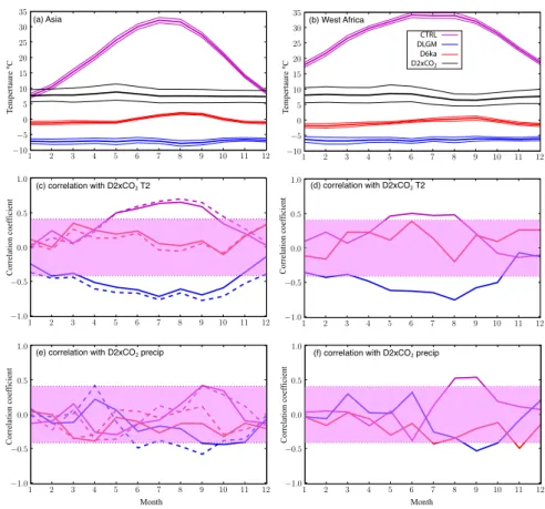
et al. use a region focussed around northern India (70– 100◦E, 20–40◦N), while Ohgaito and Abe-Ouchi use a re-gion which extends further east as far as Japan (70–140◦E, 22–40◦N). We compare results from both these regions. We also analysed the West African monsoon region (20◦W– 30◦E, 10◦N–25◦N).
Data on land for the mid-Holocene and LGM are typically taken from remnants of biological material, so may contain information on a mixture of seasonal temperature, precipita-tion and other environmental factors. In the next few years we expect researchers to move towards utilising more of this information, for example, by directly modelling the climate proxies. Therefore we present results for the monsoon cli-mate on a monthly basis. The monthly mean temperature re-sults for the different regions are shown in Fig. 7. Figure 7c, d show the correlations of monthly temperatures for CTRL, DLGM and D6ka with those for D2×CO2. The results are
similar for both regions, with the correlation being strongest for DLGM and moderate for CTRL, while there is no sig-nificant correlation for D6ka. In this case we do also find significant correlation between the CTRL and DLGM tem-peratures, suggesting that these data do not test independent aspects of the model. Figure 7e, f show the correlation of the CTRL, DLGM and D6ka temperatures with precipitation for D2×CO2. Here the results are less significant although there
CTRL
DLGM D6ka
D2xCO2
(a) Asia
(c) correlation with D2xCO2 T2
(b) West Africa
Correlation coef
ficient
Correlation coef
ficient
Correlation coef
ficient
T
empertaure
oC
Month Month
Correlation coef
ficient
(d) correlation with D2xCO2 T2
(e) correlation with D2xCO2 precip (f) correlation with D2xCO2 precip
T
empertaure
oC
Fig. 7.Correlation of monthly 2 m temperature results for the monsoon region. Left plots, Asia; solid lines, Braconnot et al. (2007a) region;
dashed lines: Ohgaito and Abe-Ouchi (2007) region. Right plots, West Africa, Braconnot et al. (2007a). (a, b)Temperatures for CTRL, DLGM, D6ka and D2×CO2.(c, d)Correlation of monthly temperature for CTRL, DLGM, D6ka with monthly temperature for D2×CO2.
(e, f)Correlation of monthly temperature for CTRL, DLGM, D6ka with monthly precipitation for D2×CO2.
shows the results for the precipitation for CTRL, DLGM and D6ka. Figure 8a, b show the precipitation for CTRL, DLGM, D6ka and D2×CO2for the two regions. It is notable here that
the changes are rather large for D2×CO2, DLGM and D6ka
when compared to the base annual cycle of the control run. All experiments, but particularly D2×CO2have a large
en-semble spread from May to October, indicating a high degree of uncertainty in the ensemble predictions. Figure 8b,c show the results for the correlations with D2×CO2 precipitation.
For Asia, only D6ka shows any significant correlation with precipitation at D2×CO2, while for Africa D6ka has
signfi-cant correlation coefficients for 7 months of the year, and the CTRL for 4 months. The correlation of the CTRL with D6ka (not shown) is only significant for the month of November.
To summarise the results for the monsoon regions, im-proving temperatures in the monsoon regions for LGM and CTRL simulations would be expected to improve future pre-dictions of temperature. For precipitation the evidence is much weaker, but the most notable feature is that, for the monsoon regions, the results for the mid-Holocene are at least as strong as those for the other epochs.
5 Discussion
For MIROC, there is evidence that improving both the pre-industrial and LGM temperatures and precipitation should influence both the estimates of climate sensitivity and global precipitation change. For estimating future changes on the zonal scale, evidence from the pre-industrial, LGM and mid-Holocene should all prove useful. Moving to the re-gional scale of the monsoon, the LGM and pre-industrial climates are clearly the most useful for improving fu-ture temperafu-tures. For the all-important prediction of the monsoon rainfall change, the evidence is less strong, but in our results, the mid-Holocene precipitation, and to a lesser extent the pre-industrial temperature and precipitation would seem to be most useful.
CTRL
DLGM D6ka
D2xCO2
(a) Asia
(c) correlation with D2xCO2 precip
(b) West Africa
Correlation coef
ficient
Correlation coef
ficient
Precipitation mm/dy
Month Month
(d) correlation with D2xCO2 precip
Precipitation mm/dy
Fig. 8. Correlation of monthly precipitation results for the monsoon region. Left plots, Asia; solid lines, Braconnot et al. (2007a) region;
dashed lines: Ohgaito and Abe-Ouchi (2007) region. Right plots, West Africa, Braconnot et al. (2007a). (a, b)Precipitation for CTRL, DLGM, D6ka and D2×CO2.(c, d)Correlation of monthly precipitation for CTRL, DLGM, D6ka with monthly precipitation for D2×CO2.
there is evidence for warmer climates compared to present in the northern latitudes of Eurasia (Tarasov et al., 1999; Bigelow et al., 2003).
One of the clearest features of the mid-Holocene climate found in proxy records is the change in vegetation type in the Sahara north of the present-day monsoon region compared to the present day. To date most climate models have not managed to reproduce this feature (Braconnot et al., 2007a and references therein). For the mid-Holocene, while there is a general increase in the monsoon precipitation and a north-ward shift in the ITCZ over Africa (Braconnot et al., 2007b), very few models (and none of our ensemble members) have produced enough of a climate change to induce significant vegetation changes in the Sahara (Braconnot et al., 2007a). It is of some concern that there should be such strong ev-idence for bias across so many models, indicating that the models do not properly represent the processes governing the mid-Holocene. If that is the case, then our finding corre-lations between the mid-Holocene and the future climate in the model-space may not translate directly for the real world, since the missing processes may overwhelm our results. On the other-hand, the fact that there is such a clear signal in the paleo-data gives us some good evidence in the past with which to validate and improve the model. Given the short-age of data for validating climate changes, and the fact that we do get a significant correlation between mid-Holocene and increased CO2climates actually suggests that further
im-proving the simulation of the mid-Holocene climate would be a suitable focus for those wishing to improve predictions of the future.
In this context is worth noting that modern GCMs do not agree on the sign of the change for future precipitation in the monsoon regions (Meehl et al., 2007), whereas those that have been run for PMIP2 do all agree on an increase for the mid-Holocene compared to present (Braconnot et al., 2007a). Despite only using a single model in our experiments, our re-sults are consistent with this. As Fig. 8a, b imply, the precip-itation changes in the monson season are all positive for the D6ka experiment, while for the D2×CO2experiment we see
both increases and decreases among the ensemble members. For the annual mean rainfall in the three monsoon regions, the precipitation change is negative for 40% of the D2×CO2
vegetation response. While previous work with MIROC3.2 has indicated that the influence of the ocean dynamics on the monsoon is not of first order importance (Ohgaito and Abe-Ouchi, 2007), recent work integrating a dynamic vege-tation model (LPJ) into the standard version of MIROC3.2 has shown that for increased CO2, the dynamic vegetation
amplifies the increase in precipitation in the monsoon regions (O’ishi and Abe-Ouchi, 2009). It is, therefore, possible that the inclusion of dynamic vegetation could bring the models closer to modelling the green Sahara at the mid-Holocene. Therefore, it would be helpful if other similar analyses could be undertaken with different models incorporating different feedbacks.
6 Conclusions
On the whole we find that the LGM, with its relatively large negative change in CO2forcing, is more likely to be useful
for constraining future climate change, despite the noise in the correlations introduced by the responses to large ice sheet changes which do not seem relevant to future climate change. For large-scale variables such as climate sensitivity, and the seasonal signal on zonal scales, analysing the behaviour of the mid-Holocene would seem to be less helpful. The one exception to this is the northern high latitude land, where at the LGM the large ice sheets causes the relation to the in-creased CO2climate change to be weak, whereas the changes
in mid-Holocene temperatures over land are, in fact, mod-erately well correlated with both climate sensitivity and the zonal changes for increased CO2. On the more regional scale
of the African and Asian monsoons, the mid-Holocene shows interesting results for the precipitation changes, although the LGM is again more relevant for temperature.
The case for continuing modelling of the mid-Holocene is supported by the availability of observational evidence which indicates climatic conditions significantly different from present in both these regions, which may be used to validate the models. There is evidence for a warmer cli-mate compared to present in the northern latitudes of Eurasia from proxy data. It is also well known that the modelled monsoon changes at the mid-Holocene are insufficiently dra-matic: there should be more rain further north, particularly in Africa (Braconnot et al., 2007a). While the caveats relating to model inadequacy mentioned in Sect. 3 should be kept in mind, because the effect of increased CO2on monsoon
pre-cipitation is highly uncertain, the mid-Holocene should not be ignored.
Acknowledgements. The authors would like to thank A. Abe-Ouchi
for encouragement and discussions which led to the development of this work, R. Ohgaito for crucial assistance with MIRCO3.2, and the two referees, M. Crucifix and A. Ganopolski for their helpful suggestions. This work was supported by Innovative Program of Climate Change Projection for the 21st Century of the Ministry of
Education, Culture, Sports, Science and Technology (MEXT), and by the Global Environment Research Fund (S-5-1) of the Ministry of the Environment, Japan.
Edited by: V. Masson-Delmotte
References
Abe, M., Shiogama, H., Hargreaves, J., Annan, J., Nozawa, T., and Emori, S.: Correlation between Inter-Model Similarities in Spatial Pattern for Present and Projected Future Mean Climate, SOLA, 5, 133–136, 2009.
Annan, J. D., Hargreaves, J. C., Ohgaito, R., Abe-Ouchi, A., and Emori, S.: Efficiently constraining climate sensitivity with pale-oclimate simulations, SOLA, 1, 181–184, 2005.
Arnold Jr., C. and Dey, C.: Observing-systems simulation experi-ments: Past, present, and future, B. Am. Meteorol. Soc, 67, 687– 695, 1986.
Berger, A.: A simple algorithm to compute long term variations of daily or monthly insolation, Tech. Rep. 18, Universit`e Catholique de Louvain, Belgium, 1978.
Bigelow, N., Brubaker, L., Edwards, M., et al.: Climate change and Arctic ecosystems: 1. Vegetation changes north of 55 N between the last glacial maximum, mid-Holocene, and present, J. Geo-phys. Res, 108, 8170, doi:10.1029/2002JD002558, 2003. Braconnot, P., Otto-Bliesner, B., Harrison, S., Joussaume, S.,
Pe-terchmitt, J.-Y., Abe-Ouchi, A., Crucifix, M., Driesschaert, E., Fichefet, Th., Hewitt, C. D., Kageyama, M., Kitoh, A., Laˆine,´ A., Loutre, M.-F., Marti, O., Merkel, U., Ramstein, G., Valdes, P., Weber, S. L., Yu, Y., and Zhao, Y.: Results of PMIP2 coupled simulations of the MidHolocene and Last Glacial Maximum -Part 1: experiments and large-scale features, Clim. Past, 3, 261– 277, 2007,
http://www.clim-past.net/3/261/2007/.
Braconnot, P., Otto-Bliesner, B., Harrison, S., Joussaume, S., Pe-terchmitt, J.-Y., Abe-Ouchi, A., Crucifix, M., Driesschaert, E., Fichefet, Th., Hewitt, C. D., Kageyama, M., Kitoh, A., Loutre, M.-F., Marti, O., Merkel, U., Ramstein, G., Valdes, P., Weber, L., Yu, Y., and Zhao, Y.: Results of PMIP2 coupled simulations of the Mid-Holocene and Last Glacial Maximum - Part 2: feed-backs with emphasis on the location of the ITCZ and mid- and high latitudes heat budget, Clim. Past, 3, 279–296, 2007, http://www.clim-past.net/3/279/2007/.
Collins, M., Booth, B., Harris, G., Murphy, J., Sexton, D., and Webb, M.: Towards quantifying uncertainty in transient climate change, Clim. Dynam., 27, 127–147, 2006.
Crucifix, M.: Does the Last Glacial Maximum constrain climate sensitivity?, Geophys. Res. Lett., 33, L18 701, doi:10.1029/ 2006GL027137, 2006.
Hargreaves, J. C., Abe-Ouchi, A., and Annan, J. D.: Linking glacial and future climates through an ensemble of GCM simulations, Clim. Past, 3, 77–87, 2007,
http://www.clim-past.net/3/77/2007/.
Joussaume, S. and Braconnot, P.: Sensitivity of paleoclimate simu-lation results to season definitions, J. Geophys. Res., 102, 1943– 1956, 1997.
Joussaume, S., Taylor, K., Bracconot, P., et al.: Monsoon changes for 6000 years ago: results of 18 simulations from the Paleocli-mate Modeling Intercomparison Project (PMIP), Geophys. Res. Lett., 26, 859–862, 1999.
Knutti, R., Meehl, G., Allen, M., and Stainforth, D.: Constraining climate sensitivity from the seasonal cycle in surface tempera-ture, J. Climate, 19, 4224–4233, 2006.
Meehl, G. A., Stocker, T. F., Collins, W. D., et al.: Global Climate Projections, in: Climate Change 2007: The physical science ba-sis. Contribution of the Working Group I to the Fourth Assess-ment Report of the IntergovernAssess-mental Panel on Climate Change, chap. 10, Cambridge University Press, Cambridge, United King-dom and New York, NY, USA, 2007.
Mitchell, J.: Greenhouse warming: Is the Mid-Holocene a good analogue?, J. Climate, 3, 1177–1192, 1990.
Murphy, J. M., Sexton, D. M. H., Barnett, D. N., Jones, G. S., Webb, M. J., Collins, M., and Stainforth, D. A.: Quantification of mod-elling uncertainties in a large ensemble of climate change simu-lations, Nature, 430, 768–772, 2004.
Ohgaito, R. and Abe-Ouchi, A.: The role of ocean thermodynam-ics and dynamthermodynam-ics in Asian summer monsoon changes during the mid-Holocene, Clim. Dynam., 29, 39–50, 2007.
O’ishi, R. and Abe-Ouchi, A.: Influence of dynamic vegetation on climate change arising from increasing CO2, Clim. Dynam., 33(5), 645–663, doi:10.1007/s00382-009-0611-y, 2009.
Russell, G., Miller, J., and Tsang, L.: Seasonal oceanic heat trans-ports computed from an atmospheric model, Dynam. Atmos. Oceans., 9, 253–271, 1985.
Schneider von Deimling, T., Held, H., Ganopolski, A., and Rahm-storf, S.: Climate sensitivity estimated from ensemble simula-tions of glacial climate, Clim. Dynam., 27, 149–163, 2006. Solomon, S., Qin, D., Manning, M., Chen, Z., et al.: Climate change
2007: The physical science basis. Contribution of the Working Group I to the Fourth Assessment Report of the Intergovernmen-tal Panel on Climate Change, 2007.
Tarasov, P., Guiot, J., Cheddadi, R., et al.: Climate in northern Eura-sia 6000 years ago reconstructed from pollen data, Earth Planet Sc. Lett., 171, 635–645, 1999.
Tsushima, Y. and Manabe, S.: Influence of cloud-feedback on an-nual variation of global mean surface temperature, J. Geophys. Res., 106, 22635–22646, 2001.
Whetton, P., Macadam, I., Bathols, J., and O’Grady, J.: As-sessment of the use of current climate patterns to evaluate re-gional enhanced greenhouse response patterns of climate models, Geophys. Res. Lett., 34, L14 701, doi:10.1029/2007GL030025, 2007.