of Classical Invariant Theory
Evgeny V. Mavrodiev*
Department of Biology, University of Florida, Gainesville, Florida, United States of America
Abstract
It has long been known that structural chemistry shows an intriguing correspondence with Classical Invariant Theory (CIT). Under this view, an algebraic binary form of the degreencorresponds to a chemical atom with valencenand each physical molecule or ion has an invariant-theoretic counterpart. This theory was developed using the Aronhold symbolical approach and the symbolical processes of convolution/transvection in CIT was characterized as a potential ‘‘accurate morphological method’’. However, CIT has not been applied to the formal morphology of living organisms. Based on the morphological interpretation of binary form, as well as the process of convolution/transvection, the First and Second Fundamental Theorems of CIT and the Nullforms of CIT, we show how CIT can be applied to the structure of plants, especially when conceptualized as a series of plant metamers (phytomers). We also show that the weight of the covariant/invariant that describes a morphological structure is a criterion of simplicity and, therefore, we argue that this allows us to formulate a parsimonious method of formal morphology. We demonstrate that the ‘‘theory of axilar bud’’ is the simplest treatment of the grass seedling/embryo. Our interpretations also represent Troll’s bauplan of the angiosperms, the principle of variable proportions, morphological misfits, the basic types of stem segmentation, and Goethe’s principle of metamorphosis in terms of CIT. Binary forms of different degrees might describe any repeated module of plant organisms. As bacteria, invertebrates, and higher vertebrates are all generally shared a metameric morphology, wider implications of the proposed symmetry between CIT and formal morphology of plants are apparent.
Citation:Mavrodiev EV (2009) Classical Morphology of Plants as an Elementary Instance of Classical Invariant Theory. PLoS ONE 4(9): e6969. doi:10.1371/ journal.pone.0006969
Editor:Nick Monk, University of Nottingham, United Kingdom
ReceivedMarch 6, 2009;AcceptedAugust 10, 2009;PublishedSeptember 11, 2009
Copyright:ß2009 Mavrodiev. This is an open-access article distributed under the terms of the Creative Commons Attribution License, which permits unrestricted use, distribution, and reproduction in any medium, provided the original author and source are credited.
Funding:The author has no support or funding to report.
Competing Interests:The author has declared that no competing interests exist.
* E-mail: [email protected]
Introduction
Classical invariant theory (CIT) studies the intrinsic or geomet-rical properties of polynomials, identifying those properties which are unaffected by a change of variables [1,2]. The mathematical parts of Introduction and all Methods outlined below are based upon [1–4].
The simplest example of a polynomial is the binary form. More accurately, the binary form is a homogeneous function of the variablesx~ðx,yÞ, which can be either real or complex:
Qð Þx ~Qðx,yÞ~X
n
i~0
ai
n i
xn{iyi ðIÞ :
The integernis the degree of the form.
Under the general transformation of variables: ðx,yÞ? a~xxzb~yy,c~xxzd~yy
ð Þ,the polynomial (I) is mapped to a new poly-nomial, given by:
~ Q
Qðxx,~~yyÞ~Qða~xxzb~y,c~y xxzd~yyÞ ðIIÞ:
Aninvariantof the binary form Q(x) is a function:
Ið Þ~aa~(det A)gIð Þa,A[GL 2ð Þ
depending on the coefficients of Q, which, up to a determinantal factor (detA), does not change (is invariant) under the action (II) of the general linear group, where:
A~ ab cd
~ad{bc
is nonsingular, i.e. an element of some general linear group GL(2). Acovariant is a function, depending both on its coefficients and on the independent variablesx= (x,y). Therefore:
Jð~aa,~xxÞ~det Að ÞgJða,xÞ,A [GL 2ð Þ
:
wheregis the weight of the invariant (or covariant). The degree of Jis its degree in the independent variables, the order ofJorIis its degree in the coefficientsaof the equation.
There are several Theorems in CIT. The most important probably are the First and the Second Fundamental Theorems, the Basis Hilbert’s Theorem and the Hilbert’s ‘‘theorem of zeros’’ (Nullstellensatz).
If the invariant or covariant is equal to zero, it vanishes, and we therefore may designate it ‘‘trivial’’. A binary formNð Þx for which all the invariants are trivial is known as a Nullform. In CIT, Hilbert’s ‘‘theorem of zeros’’ provides the criteria of the Nullforms. It has also been proved that if Q(x) is a binary form of degreen, then there are a finite number of invariants and covariants C1… CK with the property that any other covariant or invariant of Q(x) can be written as polynomial of these basic covariants and invariants (Gordan Theorem of Finiteness). Hilbert proved the more general version of Gordan’s Theorem (Basis Hilbert’s Theorem), and we may say that these basic, ‘‘irreducible’’ or ‘‘elementary’’ invariants and covariants C1… CKare a Hilbert basis of form Q(x).
It has long been known that structural chemistry shows an intriguing correspondence with CIT [1–3,5–7]. Under this view, the invariant of a system of binary forms (quadratic, cubic etc.) is the analogue of a chemical molecule composed of atoms of various valences: an algebraic binary form of the degreencorresponds to a chemical atom with valencen. Thus, each physical molecule or ion has an invariant-theoretic counterpart [2], a linear form, for example, corresponds to a hydrogen atom, a quadratic form to an oxygen atom etc. [6]. This theory was developed using the Aronhold symbolical method (see Methods) with a big number of examples [3].
From being a popular mathematical theory at the turn of the 19th and 20th centuries, the CIT gradually lost interest in the opinion of mathematicians after David Hilbert’s proof of the main theorem of this theory – the Hilbert’s Basis Theorem. As far we can judge, Hilbert never addressed Sylvester’s analogy [3,6]. However, physics have paid serious attention to this idea. For example, Born [8] based the theory of homopolar valences in multiatomic molecules on the analogy of Sylvester [6] as repre-sented in [3] and Weyel with co-authors published at least two papers [9,10] addressing this ‘‘formal, although very appealing mathematical analogy’’ [9]. Latter, Griffith [11] suggested that in his chemico-algebraic theory, Sylvester [6] had anticipated the essential and central role of a certain type of algebra in the modern theories of chemical valence, and that his theory therefore is a ‘‘partial anticipation’’ of modern quantum chemistry [11, see also 12].
The basic symbolic process of invariant building in CIT ( ‘‘Faltungsprozess’’ or ‘‘Convolution’’; see Methods) was charac-terized as an ‘‘accurate morphological method’’ [13] and previously Sylvester called the algebra of the invariants of binary forms as ‘‘Analytical Morphology in its absolute sense’’ [14]. However, CIT has never been applied to the morphology of living organisms.
Based on the morphological interpretation of binary form, as well as the process of convolution/transvection of CIT, I show here how CIT can be applied to the structure of plants, especially when conceptualized as a series of plant metamers (phytomers). Classical morphology of plants is not equal to phytonism, but the concept of phytonism is the closest allusion to the basic principle of morphology itself, to Goethe’s principle of metamorphosis, according to which one and the same organ make its appearance in multifarious forms [15]. The study of both morphology and plant development, both past and present, has widely accepted phytonism due to its accurate representation of plant form [16–29]. We also show, that classical plant morphology is an elementary instance of CIT. To do this, here we provide the morphological interpretation of two general theorems of CIT: the First and Second Fundamental Theorems. We also propose a morphological interpretation of Hilbert’s Nullform as a framework for future application of famous Hilbert’s ‘‘theorem of zeros’’ to classical morphology.
Methods
Aronhold’s symbolical method proposed, that the binary form Qð Þx is symbolically the n-th power of the linear form (or monomial):
ax
ð Þ~a1xza2y ðIIIÞ
:
Therefore we can replace Q(x) with a symbolic form:
Qð Þx~Qðx,yÞ~X
n
i~0 ai
n i
xn{i yi~X
n
i~0 n i
a1n{ia2ixn{iyi~ða1xza2yÞn~ðaxÞn
whereai~a1n{1a2i,a~ða1,a2Þ ðIVÞ:
EachQð Þx will have a corresponding symbolic form which is essentially found by replacing each coefficient by a symbolic coefficient using equation (IV). We then may call the letter aa ‘‘symbolic letter’’ or ‘‘symbol’’ of the coefficients of binary form Qð Þx .
Equation (III) is also called a ‘‘bracket factor of the first kind’’. A ‘‘bracket factor of the second kind’’ is the 262 determinant:
ab
½ ~det a1 a2 b1 b2
~a1b2{a2b1 ðVÞ:
wherea1,2andb1,2are symbolic letters.
Using the Aronhold symbolical method we may therefore re-write complicated invariants of Qð Þx as a simple sequence of bracket factors of the first and second kind. The First Fundamental Theorem of CIT states that ifJ(a,x) is a covariant of the binary form (I), then the symbolic form ofJcan always be written as a bracket polynomial P. The weight of the covariant is equal to the number of bracket factors of the second kind in any monomial of P and the degree of the covariant is the number of bracket factors of the first kind of P.
We can associate an atom with bracket factor of the first kind (III) [1–3,5–6]. The degree n of the factor of the first kind corresponds to the valence of the atom. The connection between two atoms can be described using a bracket factor of the second kind (V)[1–3]. For example, the symbolic bracket polynomial
ab
½ 2ð Þaxn{2ðbxÞn{2 describes a molecule that consists of two atoms:aandb. Since the bracket factor½aboccurs twice, there will be two bonds between atomaand atomb. So, each bracket factor of the first kindð Þaxn{2 andðbxÞn{2 corresponds ton–2 free valences of atomsaandbaccordingly [1–3].
Also, we may re-write any binary form ð Þaxn as polar forms: ax
ð Þn{1ð Þay,ð Þaxn{2ð Þay2 etc. Polar forms are comparable to atoms of non-constant valence [3].
We may symbolically transit two bracket factors of the first kind in a bracket factor of second kind [1–3] and call this transition a ‘‘Faltungsprozess’’ [3], or as a ‘‘process of convolution (‘‘Faltung’’)’’ [4] or, which is the same in our case [4], as a ‘‘transvection’’ (‘‘Uberschiebung’’) of two forms:
a,b
ð Þ?½ab
:
‘‘Convolution’’ is similar to the process of saturation for of the valences of atoms [1–3].
For convolutionða,bÞkof formsð Þaxn,ðbxÞm, this is true:
a,b
ð Þk~½abkð Þaxn{kðbxÞm{k ðVIÞ:
If k= 1 we may call equation (VI) Jacobian, and if k= 2, equation (VI) is a Hessian of two binary forms. For example, an atom of oxygen (valence = 2) corresponds to a binary form of the second degree:ðvxÞ2. The first and second convolutions of two binary formsðv1xÞ2 andðv2xÞ2therefore provide an invariant/
covariant corresponding to a hypothetical oxygen radical (the trivial covariant Jacobian½v1v2ðv1xÞðv2xÞÞand a stable neutral
‘‘molecule’’ of oxygen the invariant Hessian½v1v22
For simplicity we may call a binary form of the second degree a ‘‘binary quadratic’’ (or simply ‘‘quadratic’’), a binary form of the third degree a ‘‘binary cubic’’ (or simply ‘‘cubic’’) etc.
Results and Discussion
1. Morphological interpretation of the First Fundamental Theorem of CIT
According to the phytonic theories each organ of a plant (shoot, spikelet, flower etc.) is simply the repetition of phytomer that principally includes the stem joint, the leaf, the axillary bud/
meristem, and the secondary roots [17,20,21,23,25,27]. We also include in a phytomer the prophylls of the axillary’s bud (with hypopodium and mesopodium, if present) [21,29]. It is not necessary to always associate the bud with the leaf in whose axil it occurs [23,27,29,30].
Because each plant phytomer generally connects with two other neighbours in sequence (Figure 1A and B) and includes the bud, or, in other words, connect with the phytomer of the next order, we propose an analogy: in the simplest case the plant phytomer itself corresponds to a binary cubic (Figure 1C) and a phytomer with a reduced or non-functional axilar bud/meristem corre-sponds to the polar of a binary cubic (Figure 1C). Binary forms of degrees higher then three can represent a phytomer with serial or collateral buds/meristems. Two connected phytomers can there-fore be described by a Jacobian and (or) by a Hessian of two bracket factors of the first kind, for example, of two binary cubics. Therefore, a shoot or shoot-system built out of a chain of n phytomers will always correspond to a covariant ofnbinary forms represented by a symbolic bracket polynomial of bracket factors of the first and second kind (Figure 1D). This provides a morphological interpretation of the First Fundamental Theorem of CIT, according to which the symbolic form of covariantJ(a,x) can always be written as a bracket polynomial P of both kinds of factors [1,2,4].
Figure 1. A description of the repeated unit ofOrontium aquaticumL. (Araceae) containing five phytomers. ASchematic image ofO. aquaticum[30].B, Diagram of the repeated unit containing five phytomers [30].C, A description ofBby the covariant of five binary cubics.D, Reducible covariant of five binary cubics corresponded toB. P – prophyll; E – mesophyll; M – monopodial leaf; S – sympodial leaf; X – first phytomer of inflorescence; e – foliage leaf, c – cataphyll, s – sylleptic growth [30]. All morphological terminology and images are from [30].
The general morphological sense of the First Fundamental Theorem of CIT therefore is obvious: any morphological structure alwayscan formally be expressed in terms of the parts and the connection of these parts. In the context of phytonism, these parts are equal to phytomers.
Irreducible invariants/covariants [1,2,4] may correspond to elementary combinations of phytomers (roughly, to ‘‘articles’’ [30,31]). The invariant/covariant obviously may be reducible even though the biological structure is never found in a reduced form.
2. Morphological interpretation of the Second Fundamental Theorem of CIT
According to the Second Fundamental Theorem of CIT, any identity between bracket polynominals can be deduced from the Three Fundamental Identities [1,2]. If formal morphology is an elementary instance of CIT, all morphological problems will, in principle, resolve using three simple rules, under a morphological interpretation of the Fundamental Identities of CIT.
The First Fundamental Identity, ½ab~{½ba, states that the connection of the lowest phytomer with the uppermost one is principally equal to the opposite connection (Figure 2A) [see also 1, 2]. The Second Fundamental Identity,½abð Þcx~½ acðbxÞz½ cbð Þax, states that in the covariantðabÞð Þcx, the bracket factor of the second kind½abdescribes the connection betweenð Þax andðbxÞ, so, ifð Þax andðbxÞdescribe two connected entities, thenð Þcx, (as well as (ax) andðbxÞin the same cases), are the reduced entity, located between, above or below the connected entities. In other words, the Second Identity proposes the correct way to visualize a member which has disappeared from the sequence (Figure 2B).
According to Third Fundamental Identity of CIT,½ab½ cd~ ac
½ ½bdz½ cb½ad. The Second and Third Identities are similar [1,2,4] and in the case of so called ‘‘monostichous phyllotaxis’’ [31] it is easy to interpret the Third Identity exactly in the manner of the Second.
To make a more general interpretation (Figure 2C) clear, we need to consider that mosses, gymnosperms and angiosperms all share two basic types of stems: holocyclic and mericyclic [17,24] (Figure 3A and B). So, if½aband ½ cd described the connection between corresponded phytomers, then ½ab½ cd is an exact description of the simple mericyclic stem. The covariant½ab½ cd therefore describes the fused pairs of phytomers½aband½ cd, and the covariants½ ac½bdand½ cb½addescribe the linear sequences of corresponded phytomers, but with reduced pairs½bd(or½ ac) and ½ cb respectively (Figure 2C). The Third Identity therefore generally asserts the principal conformity of the two basic types of stem.
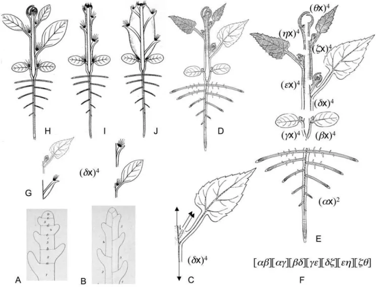
Because the lateral branch of a mericyclic stem is also mericyclic, the simplest description of the phytomer of a mericyclic stem is the binary quartic (Figure 3C). In a simplest case mericyclic stems may be therefore described using a covariants of a binary quartics. This provides a description of Troll’s bauplan of the angiosperm plant [32,33] and the principle of variable proportions (Figure 3D–J) [32,33].
3. Morphological misfits, wholeness and the Nullforms of CIT
According to Goethe, the plant body can be shown as the metamorphosis of the ‘‘Leaf ‘‘ (‘‘Blatt’’) [15]. Using CIT we may re-formulate this observation: Goethe’s ‘‘Blatt’’ corresponds to Qð Þx (or, generally, to systemfQð ÞxgÞand, therefore, phytomers
ax
ð Þn,ð Þbxn,ðgxÞn etc are seen as symbolical representations of Qð Þx
:Because a phytomer encloses all the basic organs, we may
also treatQð Þx as an entity corresponding to the whole plant, or therefore we may understand the phytomers (ax)n, (bx)n, (gx)netc. as a parts that formally represent this whole [34].
If a plant is a single whole, then it does not make sense to treat the structure of this plant in terms of a sequence of phytomers. In the context of the current approach it means that all invariants/ covariants of the formNð Þx corresponding to this plant, are equal to zero. A binary formNð Þx for which all the invariants vanish is known as a Nullform [2]. Certain morphological misfits [31, 35–37] are therefore semantically identical to the Nullforms of CIT. The shoot system of Utricularia’s species (Magnoliophyta, Lentibulariaceae) is probably, the best-known example of this kind [36,37]. Bryopsis corticulans (Chlorophyta, Bryopsidaceae) [38] is another example.
4. Elementary examples of the application of CIT to plant morphology
As shown above, the Third Identity of CIT generally asserts the principal conformity of two basic types of a stem – mericyclic and holocyclic. However due to the interpretation of the Third Identity of CIT, just the description of the mericyclic stem in notation of CIT (Figure 2C) shows that the mericyclic stem cannot be derived from the holocyclic simply by vertical congenital fusion, as Celakovsky suggested [17]. The notation of CIT itself therefore provides not only a compressed manner to describe plants, but sometimes is a way to understand the logic of the form. Another example is a Nullform that, as suggested above, helps us to understand the holistic approaches in plant morphology as a part of a more general theory.
a. General remark: the weight of invariant/covariant and
morphological simplicity. Since Aristotle simplicity is widely
considered as thesigillum veriin science [39], especially in the case of physic-chemical disciplines closely connected with math [40,41]. It is obvious, however, that in classical biology the simplicity postulate may also be a convenient instrument of method [40]. It is also widely believed that simplicity is a reliable guideline for judging the elegance of proofs [41], but like all aesthetic principles, such a criterion may be subjective [39,41]. The problem of simplicity is therefore of central importance of the epistemology of the natural sciences [39] but the concept of simplicity requires objective formulation [39,41]. This has unfortunately never been undertaken in the particular case of the morphology of living organisms.
If we describe a morphological structure in the notation of CIT, we can obviously treat the weight of the covariant/invariant that we used as a measure of the simplicity of the description. In other words, we can correspond to each combination of parts of a morphological structure not only an algebraic invariant/covariant but also some natural number, which is the weight of invariant/ covariant, the measure of its simplicity. CIT therefore helps us not to discern, but more to express the most parsimonious explanation we are looking for. Thus, if we have several alternative morphological treatments of the same structure, we can select the covariant/invariant with the minimum weight and reject the alternatives.
b. A simple example: the double-needles of the umbrella
pine. The morphology of needles of Sciadopitys (the umbrella
needle represents the paired basal segments, which arise from the scale-leaf and are fused in front of it [reviewed in 34].
From the shoot morphology ofSciadopitys[42] it is obvious that the stem of this plant is mericyclic. If the needle represents the
minimum axilar shoot with a merycyclic stem, to describe the needle we need at least three quartics. Again, the quarticðaxÞ4
correspond to the phytomer with the scale leaf, the quarticsðbxÞ4
andð Þcx4 corresponds to the phytomers of the axial shoot. The Figure 2. Three Fundamental Identitys of CIT and their morphological interpretation (A–C).The images of phytomers from [31] are re-drawn without buds, reduced phytomers being re-drawn in a dotted line.
covariant½ab½ acð Þax2ðbxÞ3ð Þcx3of weight two therefore describe the double needle of the umbrella pine.
But if the double needle of the umbrella pine is equal to one phyllome we need only one quarticð Þax4 to describe the whole needle. This quartic describes the phytomer with the appendicular part divided into scale and the paired basal segments. So we have to conclude that this treatment is more simple than the alternative one.
Both alternative treatments, however, are questionable from the pure morphological standpoint. If the needle of umbrella pine is a shoot, where are the prophylls of this shoot? In addition, Carrier [reviewed in 43] described the monstrousSciadopitysneedle where the slightly bifid character of the extremity of the ordinary needle had become very pronounced, and where a bud was developing on the interval between the two points [reviewed in 43]. If the
needle of Sciadopitys is one phyllome, how do we explain this unusual morphology of mutants?
This observation of Carrier [reviewed in 43] appears to be strong evidence that the needles ofSciadopitysrepresented deeply modified lateral shoots (‘‘phylloid shoots’’, ‘‘phylloclades’’, ‘‘clad-odes’’ etc.), perhaps with reduced prophylls. In this case the double-needle is actually composed of stem derivates.
However, if we treat the needle of the umbrella pine simple as a pair of fused transversal prophylls of the bud that are born in the axil of the scale, then we may associate these prophylls with the same scale-leaf phytomer and again describe the whole double needle ofSciadopitysonly by single quartic (ax)4. This solution is close to Engelmann and Mohl’s [reviewed in 43] solutions and to the modern concept of a double-needle [42].
Figure 3. Basic types of segmentation of a stem, descriptions of Troll’s bauplan of angiosperms and the principle of variable proportions.All imagesA–EandG–Jare re-drawn from [17] and [32] with or without modifications.A, Holocyclic stem [17] constructed from a series of phytomers each occupying the entire diameter of the axis.B, Mericyclic stem [17] constructed from a series of phytomers each occupying only a portion of the whole diameter of the axis.C, The phytomer of mericyclic stem and the corresponded binary quartic. The prophylls, the hypopodium and the mesopodium are not shown.D, The bauplan of the angiosperm plant (‘‘Urpflanze’’) [32].E, Same asD, but built up from the primary root and shoot with mericyclic stem, each phytomer is drawn with the corresponding binary quartic, primary root drawn with the corresponding binary quadratic.F, Brief notation [1] of covariant corresponded toD,E, andH–J.G–J, The principle of variable proportions [32]: the same binary form corresponds to the phytomers themselves or to the parts of the primary thickening and modified shoot axis corresponding to phytomers, that share the same position in bauplanDbut generally differ with the shape and/or proportions (G). The phytomers or corresponded parts of a shoot axis are drawn with prophylls/spines [18,32] and buds/areoles [18,32]. Each plantH(‘‘Pereskia’’, Cactaceace),I(‘‘Cylindropuntia’’, Cactaceae), andJ(‘‘Ferocactus’’, Cactaceae), as well as the bauplanDtherefore may be described by a covariant of the kindF.
If the double-needle of Sciadopitys is a pair of fused lateral prophylls, the bud observed by Carrier [reviewed in 43] represents the apex of the axial shoot, which is normally non-developed.
So, there are two simplest treatments of the morphology of needles of Sciadopitys, but only one of them explains the data concerning the Sciadopitys mutants. Note that without of the description of the needle of Sciadopitysin the notation of CIT, it would not be obvious that the two treatments are equal in terms of simplicity.
c. The axis with appendages or the chain of the
phytomers?. According to the ‘‘classical’’ theory there are
three basic plant organs: roots, stems and leaves. Stems are subdivided into nodes and internodes; leaves are only found at the nodes in a lateral position [32,33] (Figure 4A). Under this view, a monocot seedling [44] can be describe by the following covariant ½ri1½i1g1½g1i2½i2g2½g2i3½i3g3½g1w1½g2w2½g3w3ðg3xÞ
with a weight of nine (Figure 4C). Therefore, to provide a complete treatment we need a simultaneous system [3,4] of four binary forms.
Let us then make an alternative assumption, that the same seedling is constructed from phytomers (Figure 4B). Under this view, we can describe the seedling using an elementary system of binary cubics, e. g.Qð Þx~ð Þax3~ðbxÞ3~ð Þcx3;ðb,aÞ1~½baðbxÞ2ð Þax2~0;
b,a
ð Þ2~½ba2ðbxÞð Þax~H;ðH,cÞ~½ba2½ acðbxÞð Þcx2(Figure 4D). The weight of this irreducible covariant is three.
From anatomical and developmental points of view a monopodial shoot with the holocyclic stem may equally be described as a chain of phytomers or as a stem with adherent leaves [45]. Which description is simpler?
If the shoot is a stem with leaves, let us for simplicity exclude nodes and internodes and describe the stem only by one binary formð Þax2mz2. Let us also describe each of m leaves by the linear binary form (bx). In this case the covariant ½a1b½a2b. . .
amb
½ ðaxÞmz2 of weight m corresponds to the whole shoot. But
if the shoot is a chain of the phytomers ða1xÞ3,ða2xÞ3,
a2x
ð Þ3. . .ðamxÞ3, then we can describe it by the covariant
a1a2
½ ½a2a3. . .½am-1amða1XÞ2ða2XÞða3XÞ. . .ðamXÞ2of the weight m{1:
Because in case m .0, m21,m, the second description is simpler and must be accepted.
d. What solution of grass seedling is the simplest
one?. One of the most long-lasting and controversial
discu-ssions in the field of plant morphology concerns the organ homologies of the grass embryo/seedling, and since the beginning of the 19thcentury, more than 100 publications have addressed this issue [reviewed in 44, 46].
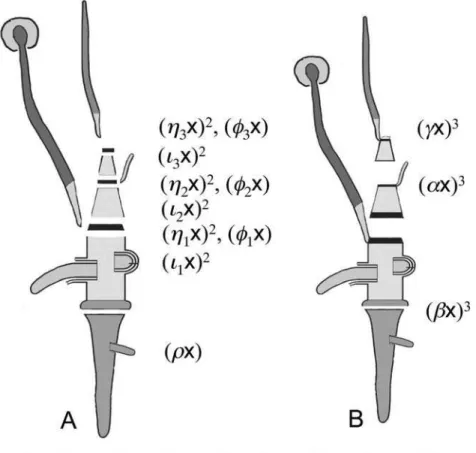
There are two classical conflicting treatments of the scutellum and coleoptile of the grass embryo: a. the coleoptile is the leaf of the plumule, the scutellum being the cotyledon (Figure 4E and F),
or b. the scutellum and coleoptile together form a single cotyledon [44,46] (Figure 4E and G).
It is not obvious which treatment simpler because in both cases the seedling contain two non-reduced, ‘‘physically present’’ phytomers (Figure 4F and G).
If the scutellum and coleoptile together form a single cotyledon (Figure 4E and G), we may describe the seedling by a Jacobian
ab
½ ð Þax2ðbxÞ2or by the Hessian ½ab2ðaxÞðbxÞ. If (ax)3 and (bx)3are equal, the Jacobian½abð Þax2ðbxÞ2is trivial. IfðaxÞ3and
bx
ð Þ3are different, the simplest description of the seedling is the Jacobian½abð Þax2ðbxÞ2.
If the coleoptile is the leaf after the cotyledon, based on the position of the coleoptile and distichous phyllotaxis (K) (diagnostic to Poaceae) we must conclude that the first leaf after the cotyledon in grasses is reduced to nothing (Figure 4F) or to the epiblast, a small scale-like structure with no vascular bundles (Figure 4E). But how does this reduced phytomer affect the complexity of the seedling? To understand this we need a correct way to visualize a member which has disappeared from the sequence. CIT, particularly the Second Identity may help us in this situation.
In the case where we treat the coleoptile as a separate leaf after the scutellum, we must describe the seedling by covariants
ab
½ 2ð ÞaxðbxÞð Þcx3 or ½abð Þax2ðbxÞ2ð Þcx3. Again ifð Þax3,ðbxÞ3, andð Þcx3 are equal, the covariant½abð Þax2ðbxÞ2ð Þcx3 vanishes, but ifð Þax3,ðbxÞ3, andð Þcx3are different, the same covariant is the simplest description of the seedling.
Based on First and Second Identities:
1:½ab
2ð ÞaxðbxÞð Þcx3~nð Þax3~ðbxÞ3~ð Þcx3o ~f½abð Þcxg2ð ÞaxðbxÞð Þcx~
~f½ acðbxÞz½ cbð Þaxg2ð ÞaxðbxÞð Þcx~ ~f½ acðbxÞz½ bcð Þaxg2ð ÞaxðbxÞð Þcx~0; 2:½abð ÞaxðbxÞð Þcx
3~
ax
ð Þ3=ðbxÞ3=ð Þcx3
n o
~½ acð Þax2ð Þcx2ðbxÞ3z½ cbð Þcx2ðbxÞ2ð Þax3
:
All descriptions of the grass seedling/embryo are summarized in Table 1. Based on this summary we must conclude that the treatment ‘‘scutellum+coleoptile = cotyledon’’ is generally more simple. This is in agreement with the current solution of the grass seedling/embryo [44].
However, if we understand the bud of the grass seedling as a lateral [23,47–50], then the coleoptile is seen to be a single prophyll [23,47–50] of the lateral bud and we may therefore treat the grass seedling as single phytomer [17,29], describe the seedling only by single cubic ðaxÞ3~ð Þaxð Þay2 and by this way
Table 1.Descriptions of grass seedling/embryo based on the different treatments of coleoptile.
ax
ð Þ3
,ðbxÞ3
,andð Þªx 3
are equal ðaxÞ3
,ðbxÞ3
,andð Þªx3are different
Coleoptile is the leaf of the plumule, the scutellum being the cotyledon
ab
½ ð Þax2b
x
ð Þ2c
x
ð Þ3~
0or½ab2a
x
ð ÞðbxÞ2c
x
ð Þ3~
0 ½abð Þax2ðbxÞ2ð Þcx3~n½ acðaxÞ2ð Þcx2ðbxÞ3z½ cbð Þcx2ðbxÞ2ð Þax3o
Scutellum and coleoptile together
form the single cotyledon ½abð Þax 2
bx
ð Þ2~0 or½ab2ðaxÞðbxÞ ½abð Þax2ðbxÞ2
demonstrate that the corresponding morphological treatment is the most simple one.
e. Conclusions and closing comments. CIT can be
applied to the structure of plants, especially when conceptualized as a series of plant metamers (phytomers). Whilst in the current study we have concentrated on the relationship between the binary form and the plant phytomer, this is the only one of many examples of the branching and repetition of the morphological and developmental units (cells, meristems, modules etc) that are omnipresent in the plant kingdom [24,35,51].
Classical morphology has largely disappeared from scientific discussions in the last ten years or so. Moreover, as Kaplan [33] correctly indicated, the discipline of plant morphology in its pure form has never been widely practiced in the United States. The basic idea of classical morphological approach, as we interpret it, is that there are general, pure mathematical laws of form that are invariant among all organisms, i. e. independent from genetics, embryology and other backgrounds. CIT provides a good opportunity to demonstrate this. Indeed, as bacteria, invertebrates, and higher vertebrates are all generally shared a metameric
morphology [52–57], much wider implications of the proposed symmetry between CIT and classical morphology of plants are apparent.
Acknowledgments
I thank Dr. Pamela S. Soltis (University of Florida), Dr. Peter Olver (University of Minnesota), Dr. Andrew N. Doust (Oklahoma State University), Dr. Samuel F. Brockington (University of Florida), and Dr. Dmitry Sokoloff (Moscow State University, Department of Physics) for reading and critics of the earlier versions of this manuscript. I am sincerely grateful to Dr. Richard Buggs (University of Florida) for linguistic correction of the text and for useful discussions that helped me to clarify arguments. I would like to thank anonymous reviewer and PLoS ONE Section Editor (Mathematics) Dr. Nick Monk for very helpful comments.
In memory of Focko Weberling ({2009)
Author Contributions
Conceived and designed the experiments: EM. Analyzed the data: EM. Wrote the paper: EM.
References
1. Olver PJ, Shakiban C (1989) Graph theory and classical invariant theory. Adv Math 75: 212–245.
2. Olver PJ (1999) Classical Invariant Theory. Cambridge: Cambridge University Press.
3. Gordan P, Alexejeff W (1900) Uebereinstimmung der Formeln der Chemie und der Invariantentheorie. Zeitschrift fur physikalische Chemie 35: 610–633. 4. Grace JH, Young A (1903) The Algebra of Invariants. Cambridge: Cambridge
University Press.
5. Clifford W (1878) Extract of a letter to Mr. Sylvester from Prof. Clifford of University College, London. Amer J Math 1: 126–128.
6. Sylvester JJ (1878) On an application of the new atomic theory to the graphical representation of the invariants and covariants of binary quantics. Amer J Math 1: 64–125.
7. Rouvray DH (1974) Isomer enumeration methods. Chem Soc Rev 3: 355–371. 8. Born M (1932) The theory of the homopolar valence in multiatomic molecules.
Angew Chem 45: 6–8.
9. Rumer G, Teller E, Weyl H (1932) Eine fu¨r die Valenztheorie geeignete Basis der bina¨ren Vektorinvarianten, Nachr Ges Wiss Go¨ttingen Math-Phy Kl . pp 499–504.
10. Weyl H (1949) Chemical valence and the hierarchy of structures. In: Weyl H, ed (1949) Philospophy of Mathematics and Natural Science - Appendix D. Princeton: Princeton Univ Press. pp 266–275.
11. Griffith JS (1964) Sylvester’s chemico–algebraic theory: a partial anticipation of modern quantum chemistry. The Math Gazette 48: 57–65.
12. Wormer PES, Paldus J (2006) Angular Momentum Diagrams. Adv Quantum Chem 51: 59–124.
13. Alexejeff W (1901) Ueber die Bedeutung der symbolischen Invariantentheorie fu¨r die Chemie. Zeitschrift fur physikalische Chemie 38: 741–743.
14. Sylvester JJ (1869) Presidential address to section A of the British Association. In: Ewald WB, ed (1869) From Kant to Hilbert: A Source Book in the Foundations of Mathematics. 2 vols. Oxford: Oxford University Press(1996) 1: 511–522. 15. Goethe JW (1952) Botanical Writings (Hawaii Univ Press, Honolulu). 16. Gaudichaud C (1841) Recherches ge´ne´rales sur l’organographie, la physiologie
et l’organoge´nie des ve´ge´taux. C R Acad Sci 12: 627–637.
17. Celakovsky LJ (1901) Die Gliederung der Kaulome. Bot Zeit 59: 79–113. 18. Velenovsky´ J (1907) Vergleichende Morphologie der Pflanzen, 2. Prag. F.
Rivinac.
19. Priestley JH, Scott LI (1935) The development of the shoot inAlstromeriaand the unit of shoot growth in monocotyledons. Ann Bot 49: 161–179.
20. Etter AG (1951) How Kentucky Bluegrass grows? Ann Mo Bot Gard 38: 293–375.
21. Galinat WC (1959) The phytomer in relation to the floral homologies in the American Maydea. Bot Mus Leafl Harv Univ 19: 1–32.
22. Nayar BK (1985) In support of phyllorhize? Curr Sci 54: 1025–1035. 23. Bossinger G, Rohde W, Lundqvist U, Salamini F (1992) Genetics of barley
development: mutant phenotypes and molecular aspects. In: Shewry PR, ed (1992) Barley: genetics, biochemistry, molecular biology and biotechnology. Wallingford: CAB International. pp 231–264.
24. Barlow P (1994) Rhythm, periodicity and polarity as bases for morphogenesis in plants. Biol Rev Cambridge Phil Soc 69: 475–525.
25. McSteen P, Leyser O (2005) Shoot branching. Ann Rev Plant Biol 56: 353–374. 26. Barthelemy D, Caraglio Y (2007) Plant architecture: a dynamic, multilevel and comprehensive approach to plant form, structure and ontogeny. Ann Bot 99: 375–407.
27. Forster BP, Franckowiak JD, Lundqvist U, Lyon J, Pitkethly I, et al. (2007) The barley phytomer. Ann Bot 100: 725–733.
28. Louarn G, Guedon Y, Lecoeur J, Lebon E (2007) Quantitative analysis of the phenotypic variability of shoot architecture in two grapevine (Vitis vinifera) cultivars. Ann Bot 99: 425–437.
29. Tzvelev NN (1997) Prophylls and phytomers as construction units of Higher Plants. Bull Moscow Soc Nat Biol Ser 102(5): 54–57 (in Russian).
30. Ray T (1987) Diversity of shoot organisation in the Araceae. Amer J Bot 74: 1373–1387.
31. Bell AD (1991) Plant Form. An Illustrated Guide to Flowering Plant Morphology, 1st edition. Oxford: Oxford University Press.
32. Troll W, Wolf KL (1950) Goethes Morphologischer Auftrag, Versuch einer Naturwissenschaftlichen Morphologie. Leipzig: Becker and Erler.
33. Kaplan DR (2001) The science of plant morphology: definition, history, and role in modern biology. Amer J Bot 88: 1711–1741.
34. Arber A (1950) The Natural Philosophy of Plant Form. Cambridge: Cambridge University Press.
35. Barlow P (1989) Meristems, metamers and modules in the development of shoot and root systems. Bot J Linn Soc 100: 225–279.
36. Richens RH (1946) Relational plant morphology. Nature 157: 127–128. 37. Rutishauser R, Isler B (2001) Developmental genetics and morphological
evolution of flowering plants, especially Bladderworts (Utricularia): fuzzy Arberian morphology complements classical morphology. Ann Bot 88: 1173–1202. 38. Kaplan DR (2001) Fundamental concepts of leaf morphology and
morphogen-esis: a contribution to the interpretation of molecular genetic mutants. Int J Plant Sci 162: 465–474.
39. Weyl H (1949) Philosophy of Mathematics and Natural Science. Princeton: Princeton Univ Press.
40. Arber A (1954) The Mind and the Eye. A Study of the Biologist’s Standpoint. Cambridge: Cambridge University Press.
41. Thiele R (2003) Hilbert’s twenty-fourth problem. Amer Math Month 110: 1–24. 42. Takaso TPB, Tomlinson PB (1991) Cone and ovule development inSciadopitys
(Taxodiaceae-Coniferales). Amer J Bot 78: 417–428.
43. Dickson A (1885) On the occurrence of foliage-leaves inRuscus(Semele)andogynus, with some structural and morphological observations. Trans Proc Bot Soc Edinb 16: 130–149.
44. Tillich HJ (2007) Seedling diversity and the homologies of seedling organs in the order Poales (Monocotyledons). Ann Bot 100: 1413–1429.
45. Schuepp O (1969) Morphological concepts: their meaning in the ideal morphology and in comparative ontogeny. Amer J Bot 56: 899–804. 46. Brown WV (1960) The morphology of the grass embryo. Phytomorphology 10:
215–223.
47. Percival J (1921) The Wheat Plant. A monograph. London: Duckworth and Co. 48. McCall MA (1934) Developmental anatomy and homologies in wheat. J Agricult
Res 48: 283–321.
49. Smirnov PA (1953) Morphological investigations of grasses. Bull Moscow Soc Nat Biol Ser 58(6): 71–75 (in Russian).
50. Jacques-Felix H (1957) Sur une interpretation nouvelle de l’embryon des Graminees. La nature axillaire de la gemmule. C R Acad Sci 245: 1260–1263. 51. Halle´ F, Oldeman RAA, Tomlinson PB (1978) Tropical Trees and Forests. An
Architectural Analysis. Berlin-Heidelberg-New York: Springer-Verlag. 52. Bateson W (1894) Materials for the Study of Variation Treated with Especial
53. Andrews JH (1998) Bacteria as modular organisms. Ann Rev microb 52: 105–126.
54. Beklemishev WN (1964) Principles of Comparative Anatomy of Invertebrates. Moscow: Nauka (in Russian).
55. Ivanov PP (1944) The primary and secondary metamery of the body. J Gen Biol 5: 61–95 (in Russian).