http://scma.maragheh.ac.ir
SOLUTION OF NONLINEAR
VOLTERRA-HAMMERSTEIN INTEGRAL EQUATIONS USING ALTERNATIVE LEGENDRE COLLOCATION
METHOD
SOHRAB BAZM
Abstract. Alternative Legendre polynomials (ALPs) are used to approximate the solution of a class of nonlinear Volterra-Hammerstein integral equations. For this purpose, the operational matrices of in-tegration and the product for ALPs are derived. Then, using the collocation method, the considered problem is reduced into a set of nonlinear algebraic equations. The error analysis of the method is given and the efficiency and accuracy are illustrated by applying the method to some examples.
1. Introduction
In this study, we consider the nonlinear Volterra-Hammerstein inte-gral equations of the form
(1.1) u(x) =f(x) + ∫ x
0
k(x, t)N(u(t))dt, x∈I := [0,1],
where u(x) is an unknown real valued function and f(x) and k(x, t) are given continuous functions defined, respectively on I and I ×I, and N(u(x)) is a polynomials of u(x) with constant coefficients. The existence and uniqueness of the solution of Eq. (1.1) are discussed in [4, 18].
Integral equations of type (1.1) arise in the mathematical modelling of parabolic boundary value problems and in various areas of physics, engineering and biological sciences [2, 8, 9, 21].
2010Mathematics Subject Classification. 65R20.
Key words and phrases. Nonlinear Volterra-Hammerstein integral equations, Al-ternative Legendre polynomials, Operational matrix, Collocation method.
Received: 01 August 2016, Accepted: 20 August 2016.
To obtain the numerical solution of integral equation (1.1), several approaches have been proposed. For example, two methods based on the use of Haar wavelets are presented in [1, 19]. Chebyshev collocation method is applied in [22] to get the solution in the domain [−1,1]. Two methods based on the operational matrices of Bernstein and Bernoulli polynomials, respectively proposed in [15] and [3]. Also, a collocation method based on the Legendre polynomials is proposed in [16]. In this paper, we use the alternative Legendre polynomials to approximate the solution of (1.1). These polynomials have recently created by Vladimir Chelyshkov [6, 7], which are orthogonal over the interval [0,1] with re-spect to the weight function w(x) = 1.
For convenience, we assume that
(1.2) N(u(x)) =um(x),
where m is a positive integer, but the method can be easily extended and applied to any nonlinear VHIE of the form (1.1), where N(u(x))is a polynomial of u(x) with constant coefficients.
The reminder of this paper is organized as follows. A review on ALPs and their properties is given in Section 2.1. Some bounds on the error of approximation of smooth functions by ALPs in L2 norm is provided
in Section 2.2. In Section 3, the operational matrices of integration and the product for ALPs is derived. In Section 4, the derived operational matrices together with the collocation method are applied to reduce the solution of integral equation (1.1) with assumption (1.2) to the solution of a nonlinear system of algebraic equations. We also show in this sec-tion that the ALP coefficient vector of funcsec-tionum(x) can be computed in terms of the ALP coefficient vector of u(x). A number of numeri-cal examples are presented in Section 5, to demonstrate the efficiency and accuracy of the proposed method. Finally, conclusions are given in Section 6.
2. Alternative legendre polynomials
In this section, we briefly introduce ALPs and give a number of theirs properties. For more details, the reader is referred to [6, 7].
2.1. Definition and properties. Let n be a fixed integer number. The set Pn ={Pnl(x)}nl=0 of alternative Legendre polynomials were
explic-itly introduced [6] as (2.1)
Pnl(x) = n−l ∑ j=0
(−1)j (
n−l j
)(
n+l+j+ 1
n−l )
It is easy to see that, in contrast to common sets of orthogonal polyno-mials, every member in bmPn has degree n.
Relation (2.1) yields Rodrigues’s type representation, (2.2)
Pnl(x) =
1 (n−l)!
1
xl+1 dn−l dxn−l
(
xn+l+1(1−x)n−l), l= 0,1, . . . , n.
It follows from (2.2) that
(2.3)
∫ 1 0
Pnl(x)dx=
1
n+ 1, l= 0,1, . . . , n.
The set Pn ={Pnl(x)}n
l=0 of alternative Legendre polynomials are
or-thogonal over the interval [0,1] with respect to the weight function
w(x) = 1, i.e. they satisfy the orthogonality relationships
∫ 1 0
Pni(x)Pnj(x)dx=
1
i+j+ 1δij, i, j= 0,1, . . . , n,
where δij denotes the Kronecker delta.
LetT denotes the transpose of a matrix or vector. By using Eq. (2.1), the ALP vector
(2.4) Φ(x) = [Pn0(x),Pn1(x), . . . ,Pnn(x)]T,
can be written in the form
Φ(x) =QX(x),
where
X(x) = [1, x, x2, . . . , xn]T,
and Qis the upper triangular matrix defined by
Q= [qkj]nk,j=0, qkj =
0, 0≤j < k,
(−1)j−k(n−k j−k
)(n+j+1 n−k
)
, k≤j≤n.
The dual matrix of Φ(x) is a diagonal matrix defined by
D= ∫ 1
0
Φ(x)ΦT(x)dx
= diag {
1 2i+ 1
}n
i=0 .
The ALPs also satisfy the three-term recurrence relation [6]
Pnn(x) =xn,
Pn,n−1(x) = 2nxn
−1−(2n+ 1)xn,
ankPn,k−1(x) = (bnkx−1−cnk)Pnk(x)−dnkPn,k+1(x),
where
ank = (k+ 1)(n−k+ 1)(n+k+ 1),
bnk =k(2k+ 1)(2k+ 2),
cnk= (2k+ 1)((n+ 1)2+k2+k), dnk =k(n−k)(n+k+ 2).
The ALPs have properties, which are analogues to the properties of common orthogonal polynomials. These polynomials are not solutions of the equation of the hypergeometric type, but they can be expressed in terms of the Jacobi polynomials Pi(α,β)(x) by the following relation
(2.6) Pnl(x) = (−1)n−lxlPn(0,2l+1)−l (2x−1), l= 0,1, . . . , n.
Hence, the ALPs are related to different families of the Jacobi poly-nomials and keep distinctively all the attributes of regular orthogonal polynomials.
Properties of the zeros of the Jacobi polynomials [20] and relation (2.6) give the following result.
Corollary 2.1 ([6]). Polynomials Pnl(x) have k multiple zeros x = 0
and n−l distinct real zeros in the interval [0,1].
By the above corollary,Pn0(x) has exactly nsimple roots in [0,1].
2.2. Function approximations and error estimates. LetH =L2(I) be the space of square integrable functions with respect to Lebesgue mea-sure on the closed interval I = [0,1]. The inner product in this space is defined by
⟨f, g⟩= ∫ 1
0
f(x)g(x)dx,
and the norm is as follows
∥f∥2 =⟨f, f⟩ 1 2
=( ∫
1
0
Let
Hn= span{Pn0(x),Pn1(x), . . . ,Pnn(x)}.
Since Hn is a finite dimensional subspace of H, then it is closed [13, Theorem 2.4-3] and for every given f ∈ H there exist a unique best approximation ¯f ∈Hn [13, Theorem 6.2-5] such that
∥f −f¯∥2 ≤ ∥f −g∥2, ∀g∈Hn.
Moreover, we have [10, Theorem 4.14]
¯
f(x) =
n ∑ k=0
fkPnk(x),
where
fk =
⟨f,Pnk⟩
⟨Pnk,Pnk⟩
= (2k+ 1)⟨f,Pnk⟩, k= 0,1, . . . , n.
(2.7)
Therefore, any function f(x) ∈ H may be approximated in terms of ALP basis as
(2.8) f(x)≃f¯(x) = ΦT(x)F,
where
F = [f0, f1, . . . , fn]T,
is the ALP coefficient vector of f. Also, any functionk(x, t)∈L2(I×I) can be similarly expanded in terms of ALP basis as
(2.9) k(x, t)≃k¯(x, t) = ΦT(x)KΦ(t),
where K = [kij]ni,j=0 is a (n+ 1)×(n+ 1) matrix in which the ALP
coefficients kij are given by
kij =
⟨⟨k,Pni⟩,Pnj⟩
⟨Pni,Pni⟩⟨Pnj,Pnj⟩
= (2i+ 1)(2j+ 1)⟨⟨k,Pni⟩,Pnj⟩, i, j= 0,1, . . . , n.
(2.10)
By the same argument as done for univariate functions, ¯k(x, t) is the unique best approximation to k(x, t) in the space
Hn2= span{Pni(x)Pnj(x), i, j= 0,1, . . . , n}.
Now, we obtain an estimation of the error norm of the best approx-imation of smooth functions of one and two variables, respectively by some polynomials in Hn and Hn2. For this purpose, let us denote by
Cm(I) the space of functions f :I →Rwith continuous derivatives
f(i)(x) = d
i
for all i such that 0≤i≤m and by Cm,n(I×I) the space of functions f :I×I →Rwith continuous partial derivatives
f(i,j)(x, t) = ∂
i+j
∂xi∂tjf(x, t), (x, t)∈I×I,
for all (i, j) such that 0≤i≤m,0≤j≤n.
Theorem 2.2. Suppose that f(x) ∈ Cn(I) and f¯(x) = ΦT(x)F be its
expansion in terms of ALPs, as described by Eq. (2.8). Then
(2.11) ∥f−f¯∥2≤
c
(n+ 1)!22n+1,
where c is a constant such that
|f(n+1)(x)| ≤c, x∈I.
Proof. Assume thatpn(x) is the interpolating polynomial tof at points xl, where xl, l = 0,1, . . . , n are the roots of the (n+ 1)-degree shifted
Chebyshev polynomial inI. Then, for anyx∈I, we have [12]
f(x)−pn(x) =
f(n+1)(ξx)
(n+ 1)!
n ∏ l=0
(x−xl), ξx ∈I.
By taking into account the estimates for Chebyshev interpolation nodes [12], we obtain
|f(x)−pn(x)| ≤ c
(n+ 1)!22n+1, ∀x∈I.
As shown in Section 2.2, ¯f is the unique best approximation of f inHn,
then we have
∥f −f¯∥22 ≤ ∥f−pn∥22= ∫ 1
0
|f(x)−pn(x)|2dx
≤
∫ 1 0
(
c
(n+ 1)!22n+1 )2
dx
= (
c
(n+ 1)!22n+1 )2
.
(2.12)
Taking the square root of both sides of (2.12) gives the result. □
Theorem 2.3. Suppose thatk(x, t)∈ Cn,n(I×I)and¯k(x, t) = ΦT(x)KΦ(t)
be its expansion in terms of ALPs, as described by Eq. (2.9). Then
∥k−¯k∥2≤
1 (n+ 1)!22n+1
(
c1+c2+
c3
(n+ 1)!22n+1 )
where c1, c2, c3 are constants such that
max
(x,t)∈I×I
∂n+1k(x, t)
∂xn+1 ≤c1,
max
(x,t)∈I×I
∂n+1k(x, t)
∂tn+1 ≤c2,
max
(x,t)∈I×I
∂2n+2k(x, t)
∂xn+1∂tn+1 ≤c3.
Proof. Assume that pn,n(x, t) is the interpolating polynomial to k(x, t)
at points (xl, tm), wherexl =tl, l= 0,1, . . . , nare the roots of the (n
+1)-degree shifted Chebyshev polynomial inI. Then, for any (x, t)∈I×I, we have [11]
k(x, t)−pn,n(x, t) =
∂n+1k(ξ, t)
∂xn+1(n+ 1)! n ∏ l=0
(x−xl)
+ ∂
n+1k(x, η)
∂tn+1(n+ 1)! n ∏ m=0
(t−tm)
− ∂
2n+2k(ξ′, η′)
∂xn+1∂tn+1(n+ 1)!2 n ∏ l=0
(x−xl) n ∏ m=0
(t−tm),
whereξ, η, ξ′, η′
∈[0,1]. Therefore, by taking into account the estimates for Chebyshev interpolation nodes [12], we obtain
|k(x, t)−pn,n(x, t)| ≤
1 (n+ 1)!22n+1
(
c1+c2+
c3
(n+ 1)!22n+1 )
,
The rest of the proof proceeds in a similar fashion to that of Theorem
2.2 □
Later, in Section 5, we will need the following theorem to evaluate the distance between the best approximation un of the exact solutionu
inHn and the computed solution ¯un.
Theorem 2.4. Let
g(x) =
n ∑
l=0
glPnl(x),
and
h(x) =
n ∑ l=0
be two functions of space Hn. Then
(2.13) ∥g−h∥2≤αn∥G−H∥2, αn= ( n
∑ l=0
1 2l+ 1
)1 2 ,
in which G and H are (n+ 1)-vectors with elements gl and hl,
respec-tively. The norm on the right hand side is the usual Euclidean norm for vectors.
Proof. We can write
∥g−h∥22 = ∫ 1
0
|g(x)−h(x)|2dx
(2.14) = ∫ 1 0 n ∑ l=0
(gl−hl)Pnl(x) 2 dx ≤ ∫ 1 0 ( n ∑ l=0
|gl−hl|2 ) ( n
∑ l=0
|Pnl(x)|2 ) dx = ( n ∑ l=0
|gl−hl|2 ) ( n
∑ l=0
∫ 1 0
|Pnl(x)|2dx )
=∥G−H∥22
( n ∑
l=0
1 2l+ 1
) .
(2.15)
Taking the square root of both sides of (2.14) gives the result. □
The previous theorem can be extended to the 2-dimensional case as follows.
Theorem 2.5. Let
k(x, t) =
n ∑ i,j=0
kijPni(x)Pnj(x),
and
s(x, t) =
n ∑ i,j=0
sijPni(x)Pnj(x),
be two functions of space Hn2. Then
∥k−s∥2 ≤α2n∥K−S∥F,
where K and S are (n+ 1)×(n+ 1) matrices with entries kij and sij,
respectively and αnis the value defined by (2.13). The norm on the right hand side is the usual Frobenius norm for matrices.
Proof. The proof proceeds in a similar fashion to that of Theorem 2.4.
3. ALP operational matrices of integration and the product
In this section, we derive the ALP operational matrices . We need the following two lemmas, which we state without proof since the proofs are easy.
Lemma 3.1. Let
Pnk(x) = n ∑ r=0
p(k)r xr,
and
Pnj(x) = n ∑ r=0
p(j)r xr,
are kth and jth ALP polynomials, respectively. Then the product of Pnk(x) and Pnj(x) is a polynomial of degree at most 2n that can be
written as
Q(k,j)2n =Pnk(x)Pnj(x) = 2n ∑ r=0
qr(k,j)xr,
where
q(k,j)r = r ∑ l=0
p(k)l p(j)r−l, r ≤n,
n ∑ l=r−n
p(k)l p(j)r−l, r > n.
Lemma 3.2. Let r be a nonnegative integer. Then
∫ 1 0
xrPnk(x)dx= n−k ∑ l=0
(−1)l(n−k l
)(n+k+l+1 n−k
)
k+l+r+ 1 , k= 0,1, . . . , n.
By combining Lemmas 3.1 and 3.2 we can easily obtain the following result.
Lemma 3.3. Let Pni(x), Pnj(x) and Pnk(x) are ith, jth and kth ALP
polynomials, respectively. If, according to Lemma 3.1, we define
Pnk(x)Pnj(x) = 2n ∑ r=0
qr(k,j)xr,
then
∫ 1 0
Pni(x)Pnj(x)Pnk(x)dx= 2n ∑ r=0
qr(k,j) n−i ∑ l=0
(−1)l(n−i l
)(n+i+l+1 n−i
In the next theorem, the ALP operational matrix of integration is first derived.
Theorem 3.4. Let Φ(x) be the ALP vector defined by (2.4). Then
(3.1)
∫ x 0
Φ(t)dt≃PΦ(x),
where P = [pkr]nk,r=0 is the ALP operational matrix of integration of
order (n+ 1)×(n+ 1), in which
pkr = (2r+ 1) n−k ∑ j=0
(−1)j(n−k j
)(n+k+j+1 n−k
) k+j+ 1
n−r ∑ l=0
(−1)l(n−r l
)(n+r+l+1 n−r
) k+r+l+j+ 2 .
Proof. By integrating ofPnk(t), i.e. Eq. (2.1), from 0 tox we get
∫ x 0
Pnk(t)dt= n−k ∑ j=0
(−1)j(n−k j
)(n+k+j+1 n−k
) xk+j+1
k+j+ 1 .
Now, using Eq. (2.8), one can approximate xk+j+1 in terms of ALPs as
xk+j+1 ≃
n ∑ r=0
bkjrPnr(x),
where, by Eq. (2.7) and Lemma 3.2, we have
bkjr = (2r+ 1) ∫ 1
0
xk+j+1Pnr(x)dx
= (2r+ 1)
n−r ∑ l=0
(−1)l(n−r l
)(n+r+l+1 n−r
) k+r+l+j+ 2 .
Therefore,
∫ x 0
Pnk(t)dt≃ n ∑ r=0
(2r+ 1) [n−k
∑ j=0
(−1)j(n−k j
)(n+k+j+1 n−k
) k+j+ 1
n−r ∑ l=0
(−1)l(n−r l
)(n+r+l+1 n−r
) k+r+l+j+ 2
]
Pnr(x)
=
n ∑ r=0
pkrPnr(x).
In the next theorem, we introduce the ALP operational matrix of the product. This matrix is of great importance in the next section where we reduce the solution of integral equation (1.1) to the solution of a set of algebraic equations.
Theorem 3.5. Let V = [v0, v1, . . . , vn]T be an arbitrary vector inRn+1.
Then
(3.2) Φ(x)ΦT(x)V ≃VˆΦ(x),
where Vˆ = [ˆvik]ni,k=0 is the ALP operational matrix of the product in
which
(3.3) ˆvik = (2k+ 1) n ∑ j=0
vjϱijk, ϱijk= ∫ 1
0
Pni(x)Pnj(x)Pnk(x)dx.
The values ϱijk in (3.3) are computed by means of Lemma 3.3.
Proof. We have
(3.4) Φ(x)ΦT(x)V = n ∑ j=0
vjPn0(x)Pnj(x)
n ∑ j=0
vjPn1(x)Pnj(x)
.. .
n ∑ j=0
vjPnn(x)Pnj(x) .
Using Eq. (2.8), one can approximatePni(x)Pnj(x), fori, j= 0,1, . . . , n,
in terms of ALPs as
Pni(x)Pnj(x)≃ n ∑ k=0
aijkPnk(x),
where, by Eq. (2.7), we obtain
aijk= (2k+ 1) ∫ 1
0
Pni(x)Pnj(x)Pnk(x)dx
So, for every i= 0,1, . . . , n, we have
n ∑ j=0
vjPni(x)Pnj(x)≃ n ∑ j=0
vj n ∑ k=0
(2k+ 1)ϱijkPnk(x)
=
n ∑ k=0
(
(2k+ 1)
n ∑ j=0
vjϱijk )
Pnk(x)
=
n ∑ k=0
ˆ
vikPnk(x).
(3.5)
Substituting (3.5) into (3.4) gives the result. □
4. Numerical solution of nonlinear VFH integral equations
In this section, we try to convert problem (1.1) with assumption (1.2) to a nonlinear set of algebraic equations. So, we consider the following integral equation
(4.1) u(x) =f(x) + ∫ x
0
k(x, t)um(t)dt, x∈I.
If we approximate functionsu(x),um(x) andk(x, t) in terms of ALPs,
as described by equations (2.8) and (2.9), then we obtain
u(x)≃ΦT(x)U,
(4.2)
um(x)≃ΦT(x)U(m),
(4.3)
k(x, t)≃ΦT(x)KΦ(t),
(4.4)
where the vectors U, U(m) and matrix K are ALP coefficients ofu(x),
um(x) and k(x, t) respectively.
In the sequel, we need to express the components of vector U(m) as nonlinear functions of the elements of the vector U. We do this by the following lemma.
Lemma 4.1. Let m be a positive integer and U and U(m) be the ALP coefficient vectors of functions u(x) and um(x), respectively. Then, we
have
(4.5) U(m) ≃ 1
n+ 1D −1Uˆm
1,
Proof. We can write
DU(m) = (∫ 1
0
Φ(x)ΦT(x)dx )
U(m)
= ∫ 1
0
Φ(x)ΦT(x)U(m)dx.
Also, using relations (4.3), (4.2) and (3.2), we have
∫ 1 0
Φ(x)ΦT(x)U(m)dx≃∫ 1 0
Φ(x)um(x)dx
≃
∫ 1 0
Φ(x)(ΦT(x)U)mdx
= ∫ 1
0
≃UΦ(x)ˆ
z }| {
(
Φ(x)ΦT(x)U) (ΦT(x)U)m
−1 dx
≃Uˆ ∫ 1
0
Φ(x)(ΦT(x)U)m
−1 dx
.. .
≃Uˆm ∫ 1
0
Φ(x)dx.
From the other side, by relation (2.2), we have
∫ 1 0
Φ(x)dx= 1
n+ 11.
Therefore,
DU(m)≃ 1
n+ 1Uˆ
m1.
Using relations (4.3), (4.4), (3.1), (3.2) and (2.5), the Volterra part of Eq. (4.1) may be written as
∫ x 0
k(x, t)um(t)dt≃
∫ x 0
ΦT(x)KΦ(t)ΦT(t)U(m)dt
= ΦT(x)K ∫ x
0
Φ(t)ΦT(t)U(m)dt
≃ΦT(x)K ∫ x
0
[
U(m)Φ(t)dt
= ΦT(x)KU[(m) ∫ x
0
Φ(t)dt
≃ΦT(x)KU[(m)PΦ(x),
(4.6)
where P is the ALP operational matrix of integration introduced in Theorem 3.4. With substituting approximations (4.2) and (4.6) into equation (4.1), we get
(4.7) ΦT(x)U ≃f(x) + ΦT(x)KU[(m)PΦ(x).
Now, by Corollary 2.1, let
(4.8) Sn={xl|Pn+1,0(xl) = 0, l= 0,1, . . . , n},
be the set of the Gauss-Chelyshkov (GC) collocation nodes. Collocating equation (4.7) at the GC nodesxl, l = 0,1, . . . , n, will result in
(4.9) ΦT(xl)U ≃f(xl) + ΦT(xl)KU[(m)PΦ(xl), l= 0,1, . . . , n.
Since U(m) is a column vector whose elements are nonlinear functions of the elements of the unknown vector U = [ui]ni=0, then equation (4.9)
is a set of (n+ 1) nonlinear algebraic equations with (n+ 1) unknowns
u0, u1, . . ., un. This nonlinear system of algebraic equations can be
solved by numerical methods such as Newton’s iterative method. If ¯U
be an approximate solution of this system, then ¯un(x) = ΦT(x) ¯U is an
approximate solution of equation (4.1).
5. Illustrative examples
introduce notations
en(x) =u(x)−un(x),
¯
en(x) =u(x)−u¯n(x),
γn=
1 (n+ 1)!22n+1, βn=∥Un−U¯n∥2,
whereu(x),un(x) and ¯un(x) are the exact solution, its best
approxima-tion using ALPs and the computed soluapproxima-tion by the presented method, respectively andUnand ¯Unare the ALP coefficient vectors ofun(x) and
¯
un(x), respectively. We also define
∥¯en∥∞= max{|¯en(xl)|, l= 0,1, . . . , n},
and the global error as [17]
ϵn=
1 |u|max
v u u t1
n n ∑
l=0
[¯en(xl)]2,
where xl,l = 0,1, . . . , n, are the GC collocation nodes defined by (4.8)
and|u|maxdenotes the maximum absolute value of the exact solution u.
Experiments were performed on a personal computer using a 2.50 GHz processor and the codes were written in Mathematica 9.
Example 5.1. Consider the following linear Volterra integral equation
(5.1) u(x) =f(x) + ∫ x
0
(x−t)u(t)dt, x∈[0,1].
The function f(x) was chosen so that the analytical solution of (5.1) is
u(x) =γxe1−γx,
with γ denoting a given (real) parameter. The results obtained for this example are given in Tables 1 and 2. Also, the error function ¯en(x) is
plotted for n= 9 in Fig. 1. We see from Table 1 that by decreasing γ, the total variation of the exact solution u(x) (which is denoted by utv)
Table 1. Computed errors∥e¯n∥∞for Example 5.1.
nγ= 1(utv = 1)γ=−1(utv =e2)γ=−2(utv = 2e3)γ=−3(utv= 3e4)
1 3.723×10⁻² 2.842×10⁻¹ 1.858×10+0 7.594×10+0
3 1.961×10⁻³ 9.313×10⁻³ 8.949×10⁻² 5.840×10⁻¹
5 1.639×10⁻⁵ 6.775×10⁻⁵ 2.256×10⁻³ 2.407×10⁻²
7 4.673×10⁻⁸ 1.714×10⁻⁷ 2.142×10⁻⁵ 4.819×10⁻⁴
9 6.407×10−112.194×10⁻¹⁰ 1.058×10⁻⁷ 5.158×10⁻⁶
Table 2. L2errors for Example 5.1 withγ=−1.
n 1 3 5 7
γn 6.25×10⁻² 3.255×10⁻⁴ 6.782×10⁻⁷ 7.569×10⁻¹⁰
∥en∥2 4.341×10⁻¹ 4.074×10⁻³ 0 0
αn 1.1547 1.29468 1.37048 1.4219
βn 4.374×10⁻¹ 1.451×10⁻² 9.275×10⁻⁵ 2.860×10⁻⁷ ∥e¯n∥2 5.578×10⁻¹ 1.390×10⁻² 8.847×10⁻⁵ 6.744×10⁻⁷
Figure 1. Graph of ¯en(x) for Example 5.1 withγ=−1 and n= 9.
Example 5.2 ([1, 14, 15]). Consider the following nonlinear Volterra integral equation
(5.2) u(x) = 3 2−
1 2e
−2x−∫ x 0
(
The exact solution of this problem is u(x) = e−x. Tables 3 and 4
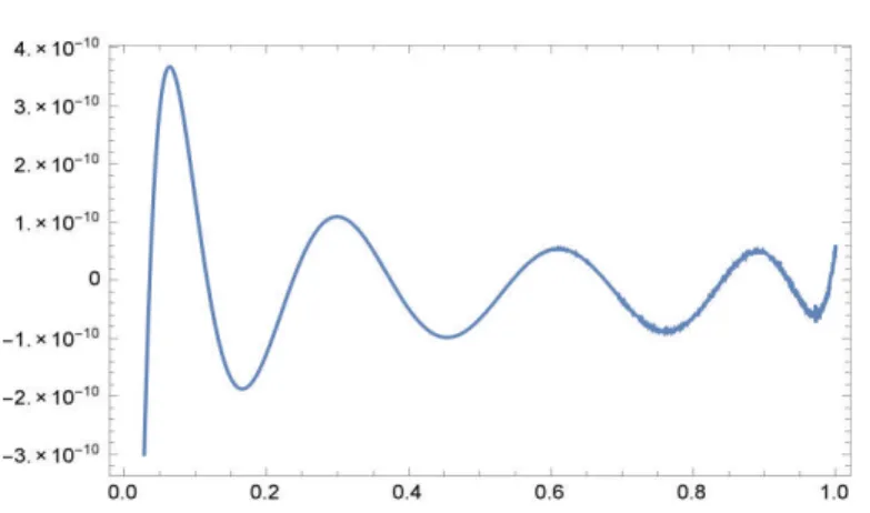
il-lustrate the numerical results obtained by the present method for this example. Also, Fig. 2 shows the graph of the error function ¯en(x)
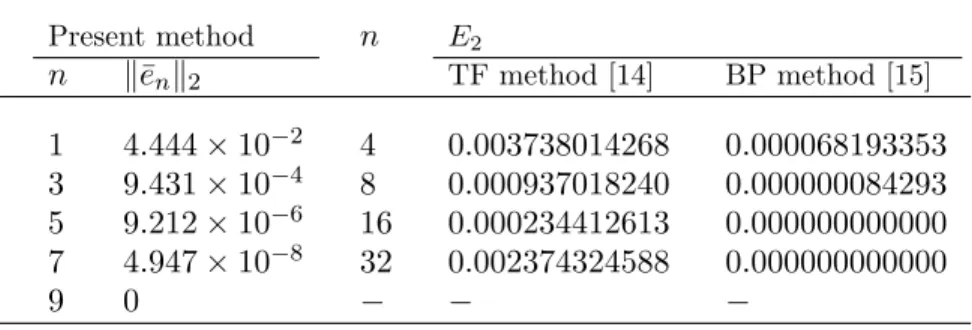
for n = 7. In Table 5, we have compared the L2 errors of the present
method with those of the triangular function (TF) method and the Bern-stein polynomial (BP) method. The table shows that better accuracy is obtained with the present method using a very fewer number of the basis functions and collocation nodes.
Table 3. L∞errors for Example 5.2. n ∥¯en∥∞
1 6.282×10⁻²
3 1.001×10⁻³
5 8.294×10⁻⁶
7 3.913×10⁻⁸
9 1.163×10⁻¹⁰
Table 4. L2errors for Example 5.2.
n 1 3 5 7
γn 6.25×10⁻² 3.255×10⁻⁴ 6.782×10⁻⁷ 7.569×10⁻¹⁰
∥en∥2 2.309×10⁻² 1.218×10⁻⁴ 0 0
αn 1.1547 1.29468 1.37048
βn 5.093×10⁻² 1.075×10⁻³ 1.009×10⁻⁵ 4.986×10⁻⁸
∥e¯n∥2 4.444×10⁻² 9.431×10⁻⁴ 9.212×10⁻⁶ 4.947×10⁻⁸
Table 5. Comparison ofL2 errors for Example 5.2. Present method n E2
n ∥en¯ ∥2 TF method [14] BP method [15]
1 4.444×10⁻² 4 0.003738014268 0.000068193353
3 9.431×10⁻⁴ 8 0.000937018240 0.000000084293
5 9.212×10⁻⁶ 16 0.000234412613 0.000000000000
7 4.947×10⁻⁸ 32 0.002374324588 0.000000000000
Figure 2. Graph of ¯en(x) for Example 5.2 with n= 9.
Example 5.3. As the final example, we consider the nonlinear Volterra integral equation
(5.3) u(x) =f(x) + ∫ x
0
(x−t)u2(t)dt, x∈[0,1].
The function f(x) was chosen so that the analytical solution of (5.3) is
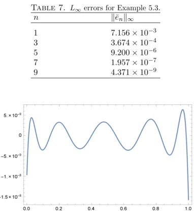
u(x) = ln(x+ 1). The results obtained for this example are given in Tables 6 and 7. Also, the error function ¯en(x) is plotted for n = 9 in
Fig. 3.
Table 6. L2errors for Example 5.3.
n 1 3 5 7
γn 6.25×10⁻² 3.255×10⁻⁴ 6.782×10⁻⁷ 7.569×10⁻¹⁰
∥en∥2 1.752×10⁻² 2.638×10⁻⁴ 1.079×10⁻⁵ 0
αn 1.1547 1.29468 1.37048 1.4219
βn 1.897×10⁻² 2.528×10⁻⁴ 6.448×10⁻⁶ 1.157×10⁻⁷
Table 7. L∞errors for Example 5.3. n ∥¯en∥∞
1 7.156×10⁻³
3 3.674×10⁻⁴
5 9.200×10⁻⁶
7 1.957×10⁻⁷
9 4.371×10⁻⁹
Figure 3. Graph of ¯en(x) for Example 5.3 with n= 9.
6. Conclusion and comments
In the presented method, the ALP operational matrices of integration and the product together with the collocation method are used to get the solution of problem (1.1) with assumption (1.2). We transformed the considered problem to a nonlinear system of algebraic equations with unknown ALP coefficients of the exact solution. As it is illustrated by the numerical examples, high accuracy results can be achieved only using a small number of basis functions.
The numerical experiments have also shown that the convergence rate of the numerical solution is similar to the ones of the best approximation of the exact solution by a polynomial in Hn.
References
2. H.O. Bakodah and M.A. Darwish,On discrete Adomian decompo-sition method with Chebyshev abscissa for nonlinear integral equa-tions of Hammerstein type, Adv. Pure Math. 2 (2012) 310-313. 3. S. Bazm,Bernoulli polynomials for the numerical solution of some
classes of linear and nonlinear integral equations, J. Comput. Appl. Math. 275 (2015) 44-60.
4. H. Brunner, On the numerical solution of nonlinear Volterra-Fredholm integral equation by collocation methods, SIAM J. Numer. Anal. 27 (1990) 987-1000.
5. H. Brunner and N. Yan,On global superconvergence of iterated col-location solutions to linear second-kind Volterra integral equations, J. Comput. Appl. Math. 67(1) (1996) 185-189.
6. V.S. Chelyshkov,Alternative Orthogonal Polynomials and Quadra-tures, Electron. Trans. Numer. Anal. 25(7) (2006) 17-26.
7. V.S. Chelyshkov, Alternative Jacobi polynomials and orthogonal exponentials, arXiv:1105.1838.
8. M.A. Darwish, Fredholm-Volterra integral equation with singular kernel, Korean J. Comput. Appl. Math. 6 (1999) 163-174.
9. M.A. Darwish, Note on stability theorems for nonlinear mixed in-tegral equations, J. Appl. Math. Comput. 6 (1999) 633-637. 10. F. Deutsch, Best approximation in inner product spaces,
Springer-Verlag, New York, 2001.
11. M. Gasca and T. Sauer, On the history of multivariate polynomial interpolation, J. Comput. Appl. Math. 122 (2000) 23-35.
12. A. Gil, J. Segura, and N.M. Temme, Numerical methods for special functions, Society for Industrial and Applied Mathematics (SIAM), Philadelphia, PA, 2007.
13. E. Kreyszig, Introductory Functional Analysis with Applications, John Wiley & Sons, 1989.
14. K. Maleknejad, H. Almasieh, and M. Roodaki, Triangular func-tions (TF) method for the solution of nonlinear Volterra-Fredholm integral equations, Commun. Nonlinear Sci. Numer. Simul. 15(11) (2010) 3293-3298.
15. K. Maleknejad, E. Hashemizadeh, and B. Basirat, Computational method based on Bernstein operational matrices for nonlinear Volterra-Fredholm-Hammerstein integral equations, Commun. Non-linear Sci. Numer. Simul. 17(1) (2012) 52-61.
16. S. Nemati, P.M. Lima, and Y. Ordokhani, Numerical solution of a class of two-dimensional nonlinear Volterra integral equations using Legendre polynomials, J. Comput. Appl. Math. 242 (2013) 53-69. 17. H. Li and H. Zou, A random integral quadrature method for
J. Comput. Appl. Math. 237(1) (2013) 35-42.
18. B.G. Pachpatte, On a nonlinear Volterra-Fredholm integral equa-tion, Sarajevo J. Math. 16 (2008) 61-71.
19. I. Singh and S. Kumar, Haar wavelet method for some nonlinear Volterra integral equations of the first kind, J. Comput. Appl. Math. 292 (2016) 541-552.
20. G. Szego, Orthogonal Polynomials, AMS, Providence, 1975. 21. A.M. Wazwaz, A reliable treatment for mixed Volterra-Fredholm
integral equations, Appl. Math. Comput. 127 (2002) 405-414. 22. C. Yang, Chebyshev polynomial solution of nonlinear integral
equa-tions, Journal of the Franklin Institute, 349 (2012) 947-956.
Department of Mathematics, Faculty of Science, University of Maragheh,, P.O.Box 55181-83111 Maragheh, Iran.