eve asholanda A Computer Program for Linear Viscoelastic by Prony Series

A COMPUTER PROGRAM FOR LINEAR VISCOELASTIC CHARACTERIZATION USING PRONY SERIES

Henrique Nogueira Silva Pedro Cavalcanti de Sousa Áurea Silva de Holanda Jorge Barbosa Soares henriquensilva@gmail.com pedro_sousa203@yahoo.com.br aurea@det.ufc.br

jsoares@det.ufc.br

Centro de Tecnologia, Departamento de Engenharia de Transportes, Universidade Federal do Ceará, Campus do Pici, 60455/760, Fortaleza - CE – Brazil

Abstract. This work describes the computer implementation and the main features of a new software that characterizes viscoelastic materials. This new proposed software is based on the representation of viscoelastic functions (relaxation modulus and creep compliance) by a Prony series, which the literature has proved to be a representative and computational efficient function for viscoelastic materials. Although the Prony series has these desired characteristics, it is not an easy task to obtain it from experimental data because it involves many numerical steps, which result in a non-practical method to be performed in a common spreadsheet software. In order to avoid such difficulties, this specific software was conceived to read experimental data and promptly output the fitted Prony series in a faster way. It was comprehensively used the object-oriented approach in C++ computer language associated with open-source wxWidgets graphical library. In order to give a general overview of the implemented code, the main classes for both numerical and graphical interface are shown. The main features available on this software are: construction of master curves; collocation method and least squares method to fit Prony series; possibility to set the independent term, the time constants and the number of dependent terms of the Prony series; and interconversion between viscoelastic functions.

1. INTRODUCTION

In mechanistic analysis of some materials the response of stresses and strains is dependent of time of loading. As examples it can be cited the asphalt concrete employed in road structures and many polymers used as primary resources in industries. These cited materials have in common the presence of an elastic (instantaneous) response associated to a viscous (time dependent) response. The theory of linear viscoelasticity is usually a viable choice to model these materials.

In this theory it is necessary to perform some stress-strain experiments involving time as a response (independent) variable. After that, the experimental results are represented by a mathematical function. On one hand, the Prony series is the most used mathematical curve to represent viscoelastic materials, which the literature has proved to be a representative and computational efficient function for such materials (Bathe, 1996; Huang, 2004; Souza, 2005; Evangelista Jr., 2006). On the other hand, the procedure to obtain Prony series from experimental data (curve fitting procedure) is not easy, involving many numerical tasks. As a consequence, it is very prone to errors if using common spreadsheet software. Another difficult task is the interconversion between viscoelastic time functions. In fact, the process of interconvertion between viscoelastic functions in time domain involves complex mathematical relations that are not easily found in current literature.

Due to these two reasons, the authors of the presented work decided to develop a computer program that perform both curve fitting of Prony series and interconversion between the viscoelastic functions in time domain. This specific software was conceived to read experimental data and promptly output the fitted Prony series in a faster way, making curve fitting of Prony series and interconversion an easier task.

The development of this proposed software was done using Object Oriented Paradigm (OOP) in C++ computer language (Stroustrup, 1997) associated with open-source wxWidgets graphical library (Smart et al., 2006). In order to give a general overview of the implemented software, the main classes for both numerical and graphical interface are shown. On a user perspective, the main features available on this software are: construction of master curves; collocation method and least squares method to fit Prony series; possibility to set the independent term, the time constants and the number of dependent terms of the Prony series; and interconversion between viscoelastic functions. In final section, the implemented features in this proposed computer program were validated.

2. BIBLIOGRAPHIC REVIEW

2.1 Prony Series

For viscoelastic materials it is necessary to consider the time-dependent response (Ferry, 1961). In a classical work Schapery (1982)shows that the time-dependent uniaxial stress σ(t) and strain ε(t) can be obtained by Eq. (1) considering this material under isothermal, nonaging e linear conditions.

∫

= =

− =

t

d d d t E t

τ

τ

τ τ

τ ε τ σ

0

) ( ) ( )

( ;

∫

=

= − =

t

d d d t D t

τ

τ

τ τ

τ σ τ ε

0

) ( ) ( )

( (1a and 1b)

Even though these material functions are obtained from experimental observation, it is necessary to represent them by mathematical functions in order to perform stress analysis on viscoelastic materials (Taylor, 1970; Evangelista Jr. et al., 2005) and to interconvert these viscoelastic functions (Park & Schapery, 1999; Park, 2001; Park & Kim, 2001). Among all analytical representations available, the Prony Series is one of the most used due to the remarkable computational efficiency associated with its exponential basis function (Park & Kim, 2001). The analytical description of relaxation modulus E(t) _{and creep} complianceD(t)by Prony series is expressed in Eq. (2):

∑

= − +

= M

i t i e

i

e E E

t E

1

)

( ρ ;

∑

=

−

− +

= N

j

t j g

j e D D

t D

1

) 1 ( )

( τ (2a and 2b)

where, Ee, ρi, Ei, and Dg, τj, Dj, are degrees of freedom of the Prony series. Equation 2a and 2b are obtained representing the viscoelastic material by a mechanical model consisting of linear springs and dashpots (Ferry, 1961; Christensen, 1982). The terms Ee and Dg are called independent terms. The exponential terms ρi and τj are known as time constants because they appear in association with the time variable t. The set of terms Ei and Dj are the dependent terms of the Prony series and the number of terms used (M and N , respectively) is determined accordlying to the experimental data. Usually, it must be used around 8 to 15 terms in Prony series of Eq. (2) in order to have a satisfactory mathematical model to be fitted from experimental data. Next section describes the most common curve fitting method to obtain the coefficients of a Prony series.

2.2 Classical Techniques for Prony Series Curve Fitting

The curve fitting of Eq. (2) from experimental data results in a nonlinear optimization problem, in which techniques of nonlinear optimizations must be applied. To solve this problem, Baumgaertel & Winter (1989) presented a nonlinear regression technique in whichρi, Ei (or τj,Dj) and the number of terms M (or N ) are all variables. However, a more common practice is to avoid the nonlinear system of equations by estimating the time constants ρi (or τj) from the total range of time domain (Schapery, 1961; Schapery, 1982; Sousa & Soares, 2007). In a classical work, Schapery (1961) proposed the selection of one ρi (or τj) for each logarithmic decade of time, resulting in a linear system of equations to find the dependent coefficients Ei (or Dj). Furthermore, as illustrated by Sousa & Soares (2007), the independent term Ee (orDg) can be directly inferred from the minimum value using a simple scatter plot of experimental data.

Once this simplified method of estimating time constants is chosen, a technique to build the linear system must be defined. In recent works (Sousa & Soares, 2007, Sousa et al., 2008), it was illustrated the classical collocation curve fitting method (Schapery, 1961), in which sampling discrete times tk are conveniently taken to be tk =aρk(or=aτk) (k=1,...,Nor M ) where typically a=1 or a=1/2 is used (Park & Schapery, 1999). An alternative method is to consider all experimental data as part of the sampling points tk(now k=1,...,P where P is the number of experimental points) resulting in the least squares method. Considering Prony series of Eq. (2) in the least squares method results in Eq. (3) and Eq. (4) for relaxation modulus and creep compliance, respectively.

i j

ijE B

(

)(

)

∑

= − − ₋ − = P k t t ij j k i k _e e A 1 / / 1

1 τ τ

(

)

(

)

∑

= − − − = P k t g k i i k e D t D B 1 / 1 ) ( τ i j

ijE B

A = (summed on j; i=1,...,N; j=1,...,N) (4) where:

(

)

(

)

∑

= − − = P k t t ij j k i k e e A 1 /

/ρ ρ

(

)

(

)

∑

= − − = P k t e k i i k e E t E B 1 / ) ( ρ

It must be emphasized that this last method (least squares method) is less sensible to the noisy of experimental data, once it considers all experimental points (k=1,...,P), rather than the small quantity of sampling points in collocation method (k=1,...,Nor M ).

2.3 Interconversion between Viscoelastic Properties

Many works about linear viscoelastic theory (Ferry, 1961; Christensen, 1982; Schapery, 1982; Park & Schapery, 1999) cite that interconversion between viscoelastic materials may be necessary due two reasons: i) the response of a material under a certain excitation condition is inaccessible in direct experiments and may be predicted from measurements under other readily realizable conditions, and ii) a material function often cannot be determined over the complete range of its domain from a single excitation and then the range can be extended by combining the responses to different types of excitation. For more details about these advantages the reader is referred to Park & Schapery (1999) and Medeiros Jr. (2006).

Park & Schapery (1999) describe an analytical approach in which the source (known) and target (unknown) functions are represented by Prony series of Eq. (2). In this work, it is shown the reduction of the interconversion from relaxation modulus E(t) (source function) to creep compliance D(t) (target function). In this reduction it is necessary to put Eq. (2a) and Eq. (2b) into the integral relation defined according to Eq. (5).

1 ) ( ) ( 0 = −

∫

t d

d dD t

E τ

ττ

τ (t>0) (5)

Considering that the time constants of the target function τj are known, the final relation to obtain the dependent terms Dj of creep compliance D(t)(target function) from the relaxation modulus E(t) (source function) is expressed according to Eq. (6).

k j

kjD B

       ≠ − − + − = + − = − − = − = − −

∑

∑

i j t t M

i i j

i i t e M i i j t j k i t e kj j k i k j k i k j k e e E e E e t E e E A ρ τ τ ρ ρ ρ τ τ τ ρ τ ρ τ when ) ( ) 1 ( or when ) 1 ( ) / ( ) / ( 1 ) / ( 1 ) / ( ) / ( and       +       + − =

∑

∑

= = − M i i e M i t i e

k E Ee E E

B k i

1 1 ) / ( 1 ρ

In the interconversion process, differently from the curve fitting process, sampling few points in the collocation method imply in results as good as the least squares method (Park & Schapery, 1999). So index k has a maximum value Q , where Q=M or N in collocation method and Q=P' in least squares method (P' is a subset of the P experimental points). The inverse interconversion process, i.e. interconversion from creep compliance D(t) (source function) to relaxation modulus E(t) (target function), is done by using the relationship described according to Eq. (7).

1 ) ( ) ( 0 = −

∫

t d

d dE t D τ τ τ

τ (t>0) (7)

Following similar method describe in (Park & Schapery, 1999), the authors of this presented work obtained the equation to find the dependent terms Ei of the relaxation modulus E(t)(target function) modulus from the creep compliance D(t)(source function). This relation is expressed according to Eq. (8)

k i

kiE B

A = (summed on i; i=1,...,M ; k =1,...,Q) (8) where:         ≠ − − + − − + − − = + − − + − − =

∑

∑

∑

∑

= = − − − − = − = − − j i N j N j t t i j j j t j t g j i N j t i k j N j t j t g ki i k j k i k i k j k i k i k e e D e D e D e t D e D e D A τ ρ ρ τ τ τ ρ ρ ρ τ ρ ρ τ ρ ρ n whe ) ( ) 1 ( ) 1 ( or n whe ) 1 ( ) 1 ( 1 1 ) / ( ) / ( ) / ( ) / ( 1 ) / ( 1 ) / ( ) / ( g N j t j g

k D D e D

B k j

      − + − =

∑

= − 1 ) / ( ) 1 ( 1 τ

3. DESCRIPTION OF THE PROPOSED COMPUTER PROGRAM

This section gives an overview of the proposed computer program. Its development was motivated due to the lack existent between linear viscoelastic theory and practical tools to use such theory. Although the algorithmic process of curve fitting Prony series and interconversion between viscoelastic functions may be done in a common spreadsheet computer program, it is important to say that such procedures are not easy to be done in this environment because: i) it involves many steps (resulting in a non-practical approach); and ii) it involves many indices (resulting in a very prone error approach).

The development of the proposed computer program, named ViscoTool, was based on the object-oriented C++ computer language, which enables data encapsulation, a more organized code and natural expansion of this code (Stroustrup, 1997; Prata, 2005). In first part of this section a short description of the main classes of ViscoTool is done. The second part describes the main features of ViscoTool from user perspective.

3.1 Development of ViscoTool Computer Program

In order to develop a computer program that performs constitutive characterization of viscoelastic materials, it was decided to use the Object-Oriented Paradigm (OOP). The main advantages of such paradigm are: i) data encapsulation (data hiding) by a class entity and ii) more natural reuse of code by class inheritance mechanisms (Stroustrup, 1997; Prata, 2005). In ViscoTool, it was not necessary to use class inheritance, but it was used extensively data hiding by class definition, which resultsin a more organized source code and easier to expand software. It was decided to use C++ language, one of the most popular OOP computer languages, associated with the graphical user interface library wxWidgets (Smart et al., 2007). This library is free-to-use, open source and a good option to developers in C++ language. Furthermore, the authors used DialogBlocks (Smart, 2007), a Rapid Application Development (RAD) tool which enable wxWidgets graphical interface code generation by graphical means, resulting in a very productive development of source code related to graphical interface.

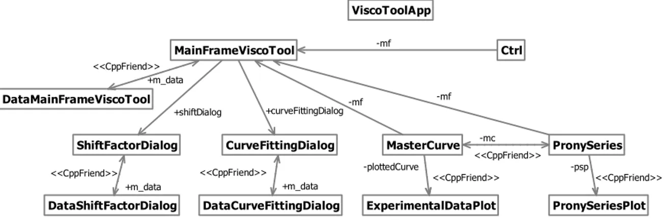
The main classes of ViscoTool are shown in Fig. 1, using the UML notation (OMG, 1997). In the next topics, the main classes related to graphical interface and numerical aspects described in section 2 (bibliographic review) are presented.

Graphical Classes of ViscoTool

The ViscoToolApp class is responsible to the initialization of the program (as main function is necessary for console applications), and instantiates the main user graphical interface class, named MainFrameViscoTool. This later one is responsible to the initial screen of ViscoTool, which has the controls (menus, toolbar) and a plotting area, for the visualization of the Prony series. As indicated in Fig. (1), the data of this class is designed in another specific class (DataMainFrameViscoTool class). The connection between the graphical class (MainFrameViscoTool) and its data class (DataMainFrameViscoTool) is done with a friendship relation between them. This design is suggested by the work of Smart et al. (2006), to provide a more modular code, separating source code of graphical controls from code of data structure. Another two graphical classes were implemented (ShifFactorDialog and CurveFittingDialog classes); and they represent minor dialogs for user interaction. The communication to the MainFrameViscoTool class is by efficient pointer mechanism, and MainFrameViscoTool has access of ShifFactorDialog and CurveFittingDialog data only using the accessors (set and get), which is a realization of the data hiding mechanism (Prata, 2005). In these two minor graphical classes it was also used data isolation from graphical controls.

Numerical Classes of ViscoTool

For the numerical implementation of curve fitting of Prony series and interconversion between relaxation modulus and creep compliance functions, it was designed three classes. The first one, the Ctrl class, is a static class that manages the numerical (non-graphical) aspects of ViscoTool. The Ctrl class is the unique way that MainFrameViscoTool class can pass information to other numerical classes, and it is done by static definition as suggested in Holanda et al. (2006).

3.2 Available Features of ViscoTool from User Perspective

From a user perspective, the proposed computer program was created to read a simple input text file where experimental data is divided into different blocks, organized by temperature in which the laboratory test was performed (Sousa et al., 2008). These blocks are structured in two different columns: (i) time column and (ii) the viscoelastic property column. It is important to say that, before the creation of this input file, a pre-treatment of data outside Viscotool might be required to exclude outliers. For illustration purposes, Fig. (2a) shows a hypothetic example of an input file for the creep compliance test. For each constant temperature indicated by the symbol “%” (the sentinel character for reading purpose), there is a list of time t and the corresponding creep compliance property.

(a)

(b)

(c) Figure 2 – input file (a, b) and output file (c) of ViscoTool.

Once the input file is loaded, a message window pops up (Fig. 2b) confirming the correct reading of input data and a plot of experimental curves is shown (see Fig. 3). After performing the required tasks, the user has the option to save the results in a text file, as indicated in Fig. (2c).

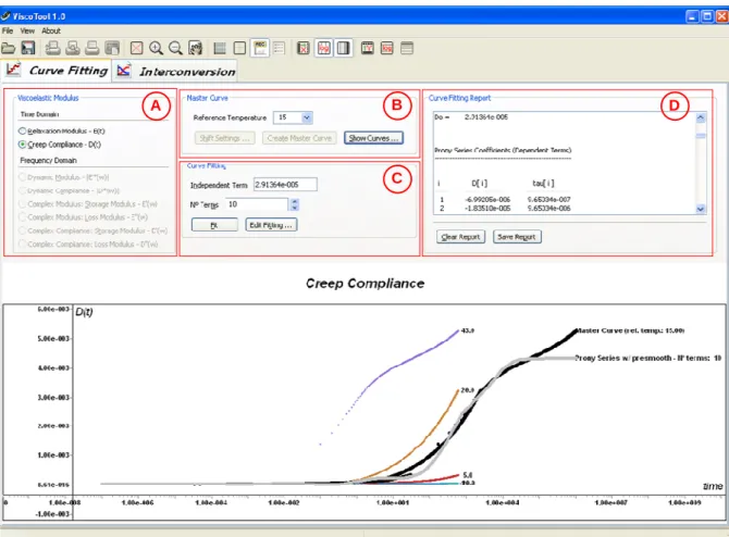
The next step concerns of fitting a Prony series from the generated master curve as indicated in Fig. (4c). ViscoTool suggests to the user both the number of terms of the Prony series (Mor N) and the value for the independent term (Ee or Dg). Such independent term is determined based on the master curve (usually the minimum value of this curve). In button “Edit Fitting” of Fig. (4c) the user has the possibility to decide which curve fitting method use (collocation menthod or least squares method). Figure (5) shows the dialog that appears when the user clicks on this button. In this dialog, the user can also edit the time constants, which sometimes solve local problems of numerical values of the viscoelastic function due to scatter of experimental measurements (Park and Schapery, 1999).

After solving the linear system, as indicated Fig. (4d), a report is created showing the selected settings and the fitted coefficients of Prony Series - Ee,ρiandEi _{for relaxation} modulusE(t); and Dg,τjandDjfor creep complianceD(t). In this report, it is showed the corresponding interconverted viscoelastic function. The user has the possibility to choose the curves to be shown (Fig. 4b) and to fit as many Prony series she/he judges necessary.

A B

C

D

(a)

(b)

(c)

(d)

Figure 4 – (a) choice of viscoelastic property; (b) master curve construction; (c) basic settings of curve fitting of Prony series; (d) report of Prony series curve fitting and interconversion.

Figure 5 – choice of curve fitting method and edition of time constants of Prony series.

A B

C

4. VALIDATION OF VISCOTOOL

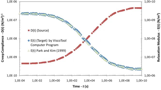
In order to validate curve fitting method and interconversion of ViscoTool, it was extracted the Prony series indicated in the work of Park and Schapery (1999). In fact, this work does not show any experimental data, but, from the Prony series given in this paper, it was simulated experimental points, making an input file to be loaded in ViscoTool. This approach is valid because the main purpose of the presented work is to validate the implementation efforts, and the fenomenological analysis of this result is irrelevant. To illustrate the inverse process shown in Park and Shapery (1999) the creep compliance curve fitting was performed as well as the corresponding interconverted relaxation modulus.

4.1 Curve Fitting using Prony series

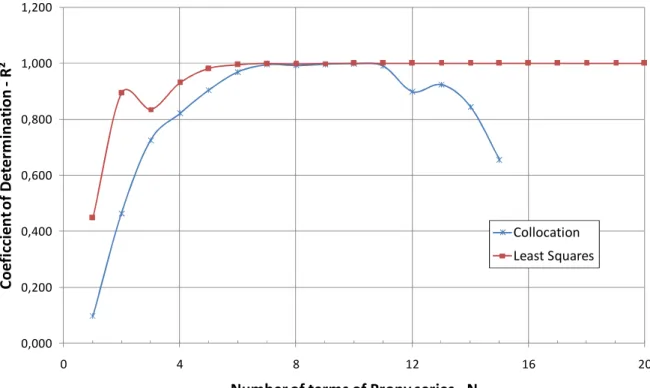
Performing the curve fitting for many terms and both process (collocation and least squares) we obtain Fig. (6). In this figure we can see that both methods can be used to curve fitting procedure, once they result in coefficient of determination very close to 1.0. This is particularly true when using 7 to 11 terms of the Prony series of Eq. (2a), which is the recommended range of terms used in Prony series in this particular example. This figure indicates also that the least squares is a more robust technique than the collocation approach, resulting in more accurate results in all domain (number of terms) and not affected by the exceeded quantity of terms used ( N from 12 to 20 terms).

0,000 0,200 0,400 0,600 0,800 1,000 1,200

0 4 8 12 16 20

C

o

e

fi

cc

ie

n

t

o

f

D

e

te

rm

in

a

ti

o

n

-R

²

Number of terms of Prony series - N

Collocation

Least Squares

Figure 6 – Coefficient R² versus number of terms of Prony series (for both collocation and least squares method).

(1999). The same accuracy in fitting using collocation method was obtained and it will not be shown here for brevity purposes.

Figure 7 – Prony series plotted in ViscoTool (N = 11) Table 1 – Prony series of creep compliance

using least squares method in ViscoTool.

j

j

D

(N/m²)-1

j

τ

(s)

1 4.08E-11 2.19E-2

2 7.37E-11 2.34E-1

3 2.25E-10 2.88E+0

4 6.40E-10 3.80E+1

5 2.03E-9 5.25E+2

6 6.86E-9 6.61E+3

7 2.19E-8 6.03E+4

8 6.50E-8 5.89E+5

9 1.37E-7 4.27E+6

10 6.93E-8 2.57E+7

11 1.45E-7 2.95E+8

g

D = 4.47E-10

4.2 Interconversion of Viscoelastic Properties

(source) to relaxation modulus (target) was correctly done, indicating that Eq. (8) was correctly obtained by authors of this current work.

Table 2 – Prony series of interconverted relaxation modulus using ViscoTool.

i E_i

(N/m²)

i

ρ

(s)

1 2.05E+8 2.19E-2

2 3.13E+8 2.34E-1

3 6.39E+8 2.88E+0

4 6.41E+8 3.80E+1

5 3.26E+8 5.25E+2

6 7.75E+7 6.61E+3

7 2.13E+7 6.03E+4

8 8.83E+6 5.89E+5

9 8.85E+5 4.27E+6

10 8.64E+5 2.57E+7

11 9.28E+5 2.95E+8

e

E = 2.23E+6

For validation purposes, Fig. (8) indicates also the interconverted relaxation modulus exhibited in the work of Park and Schapery (1999). Although this cited work presents a more accurate way to obtain the time constants, we can graphically conclude that the simplified method implemented in ViscoTool of equal time constants in both source and target functions is good enough.

1,0E+06 1,0E+07 1,0E+08 1,0E+09 1,0E+10

1,0E-10 1,0E-09 1,0E-08 1,0E-07 1,0E-06

1,0E-04 1,0E-02 1,0E+00 1,0E+02 1,0E+04 1,0E+06 1,0E+08 1,0E+10

C

re

e

p

C

o

m

p

li

a

n

ce

-D

(t

)

(N

/m

²)

-1

R

e

la

x

a

ti

o

n

M

o

d

u

lu

s

-E

(t

)

(N

/m

²)

Time -t(s) D(t) (Source)

E(t) (Target) by ViscoTool Computer Program

E(t) Park and Kim (1999)

5. FINAL REMARKS

In this work, it was presented a computer program that performs curve fitting of Prony series and interconversion between viscoelastic functions. The main features of this proposed computer program from developers and users perspective were depicted. From developer’s point of view, this computer program was designed and implemented using Object Oriented Paradigm, by using extensively class definition for data hiding and well defined communication process between these classes. From a user’s perspective, this software perform curve fitting of Prony series and interconversion between viscoelastic functions. The specialized environment constructed enables perform these numerical procedures in a more easy way than in a common spreadsheet software.

In fact other features must be implemented in this software, such as curve fitting and interconvertion in the frequency domain. This software must be viewed as an initial effort to make theory of viscoelasticy more practical to be used in characterization of materials that present time dependent mechanical responses.

Acknowledgements

The authors acknowledge to CNPq-Brazil due to the assistantship conceded to the first two authors of this work and PETROBRAS and FINEP due to the financial support of pavement analysis research.

REFERENCES

Bathe, K. J., Finite Element Procedures, Prentice Hall, 1996.

Baumgaertel, M. & Winter, H. H., 19898. Determination of discrete relaxation and retardation time spectra from dynamic mechanical data. Rheologica Acta, vol. 28, pp. 511–519. Buttlar, W. G., Roque, R. & Reid, B., 1998. Automated procedure for generation of creep

compliance master curve for asphalt mixtures. Transportation Research Record, vol. 1630, pp. 28–36.

Christensen, R. M., 1982. Theory of Viscoelasticity. Academic Press, New York, USA, 1982. Evangelista Jr., F., 2006 Análise Quasi-Estática e Dinâmica de Pavimentos Asfálticos, MSc

thesis, Programa de Mestrado em Engenharia de Transportes, Universidade Federal do Ceará, Fortaleza, Brazil.

Evangelista Jr., F., Parente Jr., E. & Soares, J. B., 2005. Viscoelastic and Elastic Structural Analysis of Flexible Pavements, In: Proceedings of XXVI Iberian Latin-American Congress on Computational Methods in Engineering (CILAMCE), Guarapari, Brazil. Ferry, J. D., 1961. Viscoelastic Properties of Polymers, John Wiley & Sons Inc.

Holanda, A. S., Parente Jr., Araújo, T. D. P., Melo, L. T. B., Evangelista Jr., F. & Soares, J. B., 2006. An object oriented system for finite element analysis of pavements. In: III European Conference on Computational Mechanics Solids, Structures and Coupled Problems in Engineering, Lisbon, Portugal.

Huang, Y. H., 2004. Pavement Analysis and Design. Pearson Education, Inc., Upper Saddle River, NJ, USA.

Medeiros Jr., M. S., 2006. Estudo de Interconversão entre o Módulo Complexo e a Creep Compliance na Caracterização de Misturas Asfálticas, MSc thesis, Programa de Mestrado em Engenharia de Transportes, Universidade Federal do Ceará, Fortaleza, Brazil.

Park, S. W., Schapery, R. A., 1999. Methods of interconversion between linear viscoelastic material functions. Part I – a numerical method based on Prony series. International Journal of Solids and Structures, vol. 36, pp. 1653–1675.

Park, S. W., 2001. Analytical modeling of viscoelastic dampers for structural and vibration control. International Journal of Solids and Structures, vol. 38, pp. 8065–8092.

Park, S. W. & Kim, Y. R., 2001. Fitting prony-series viscoelastic models with power law presmoothing. Journal of Materials in Civil Engineering, vol. 13 (1), pp. 26–32.

Prata, S., 2005. C++ Primer Plus. Fifth edition, Sams Inc., Indiana, USA.

Schapery, R. A., 1961. A simple collocation method for fitting viscoelastic models to experimental data. Rep. GALCIT SM 61-23A, California Institute of Technology, Pasadena, USA.

Schapery, R. A., 1982. Theory of viscoelasticity, Lecture notes.

Smart, J., Hock, K., Csomor, S., 2006. Cross-Platform GUI Programming with wxWidgets, Prentice Hall, USA.

Smart J., 2007. Anthemion Software Ltd.

Smart, J., Roebling, R., Zeitlin, V., Dunn, R., 2007. wxWidgets 2.8.6: A portable C++ and Python GUI toolkit.

Sousa, P. C. & Soares, J. B., 2007. Método da colocação para obtenção de séries de Prony usadas na caracterização viscoelástica de materiais asfálticos, In: XXI Congresso de Pesquisa e Ensino em Transportes - ANPET, Rio de Janeiro, Brazil.

Sousa, P. C., Silva, H. N. & Soares, J. B., 2008. Prony Series Study for Viscoelastic Characterization of Asphalt Mixtures. In: 19° Encontro de Asfalto, Instituto Brasileiro de Petróleo, Gás e Biocombustíveis – IBP, Rio de Janeiro, Brazil.

Stroustrup, B., 1997. The C++ Programming Language, Third edition, Addison-Wesley. Souza, F. V., 2005. Modelo Multi-Escala para Análise Estrutural de Compósitos

Viscoelásticos Suscetíveis ao Dano, Dissertação de Mestrado, Programa de Mestrado em Engenharia de Transportes, Universidade Federal do Ceará, Fortaleza.

Taylor, R. L., Gerald K. S. P., Goudreau, L., 1970. Thermomechanical analysis of viscoelastic solids. International Journal for Numerical Methods in Engineering, vol. 2, n. 1, pp. 45– 59.