www.atmos-chem-phys.net/9/865/2009/
© Author(s) 2009. This work is distributed under the Creative Commons Attribution 3.0 License.
Chemistry
and Physics
Quantification of the impact of climate uncertainty on regional
air quality
K.-J. Liao1, E. Tagaris1, K. Manomaiphiboon1,4, C. Wang2, J.-H. Woo3,5, P. Amar3, S. He3, and A. G. Russell1
1School of Civil and Environmental Engineering, Georgia Institute of Technology, Atlanta, GA, USA
2Joint Program on the Science and Policy of Global Change, Massachusetts Institute of Technology, Boston, MA, USA 3Northeast States for Coordinated Air Use Management (NESCAUM), Boston, MA, USA
4Joint Graduate School of Energy and Environment, King Mongkut’s University of Technology Thonburi, Bangkok, Thailand 5Department of Advanced Technology Fusion, Konkuk University, Seoul, Korea
Received: 18 January 2008 – Published in Atmos. Chem. Phys. Discuss.: 21 April 2008 Revised: 17 December 2008 – Accepted: 2 January 2009 – Published: 3 February 2009
Abstract. Uncertainties in calculated impacts of climate forecasts on future regional air quality are investigated us-ing downscaled MM5 meteorological fields from the NASA GISS and MIT IGSM global models and the CMAQ model in 2050 in the continental US. Differences between three fu-ture scenarios: high-extreme, low-extreme and base case, are used for quantifying effects of climate uncertainty on re-gional air quality. GISS, with the IPCC A1B scenario, is used for the base case simulations. IGSM results, in the form of probabilistic distributions, are used to perturb the base case climate to provide the high- and low-extreme scenarios. Impacts of the extreme climate scenarios on concentrations of summertime fourth-highest daily maximum 8-h average ozone are predicted to be up to 10 ppbV (about one-seventh of the current US ozone standard of 75 ppbV) in urban areas of the Northeast, Midwest and Texas due to impacts of mete-orological changes, especially temperature and humidity, on the photochemistry of tropospheric ozone formation and in-creases in biogenic VOC emissions, though the differences in average peak ozone concentrations are about 1–2 ppbV on a regional basis. Differences between the extreme and base scenarios in annualized PM2.5levels are very location depen-dent and predicted to range between−1.0 and+1.5µg m−3. Future annualized PM2.5is less sensitive to the extreme cli-mate scenarios than summertime peak ozone since precipita-tion scavenging is only slightly affected by the extreme cli-mate scenarios examined. Relative abundances of biogenic VOC and anthropogenic NOxlead to the areas that are most responsive to climate change. Overall, planned controls for decreasing regional ozone and PM2.5levels will continue to
Correspondence to:A. G. Russell ([email protected])
be effective in the future under the extreme climate scenar-ios. However, the impact of climate uncertainties may be substantial in some urban areas and should be included in assessing future regional air quality and emission control re-quirements.
1 Introduction
emissions remain constant. Sanderson et al. (2003) predict a 10–20 ppbV increase in ozone concentrations during July due to a combined effect of changes in vegetation and pre-scribed IPCC IS92a CO2emissions in 2090s compared with 1990s over the majority of the US.
The objective of this study is to investigate how uncer-tainties inherent in climate change forecasts impact regional air quality predictions over the continental US using mul-tiple climate futures. Given that model inputs (e.g., re-gional meteorology and precursor emissions) and parameter-izations/assumptions lead to uncertainties in regional down-scaling of future climate and air quality modeling (which have been presented elsewhere, e.g., Bergin et al., 1998; Rus-sell and Dennis, 2000; Hanna et al., 2001; Hanna et al., 2005; Gustafson and Leung, 2007), the purpose of this study is not to specifically forecast future air quality but to quantify the impact of climate uncertainties on regional air quality fore-casts, particularly focusing on ground-level ozone and PM2.5 (particulate matter with an aerodynamic diameter less than 2.5µm) due to their adverse health-related effects (Bernard et al., 2001; Galizia and Kinney, 1999; Johnson and Graham, 2005). Of particular interest are the uncertainties associated with the “climate penalty” (increases in levels of air pollu-tants caused by climate change, Mickley et al., 2004) and investigating if uncertainties in climate predictions suggest alternative emission control strategies.
2 Method
2.1 Downscaling of global climate models to a meso-scale meteorological model
The meso-scale meteorological model, MM5 (The Fifth-Generation NCAR/Penn State Mesoscale Model) (Grell et al., 1994; Seaman, 2000), is used to downscale outputs from the NASA Goddard Institute of Space Studies (GISS) global climate model (GCM) (Rind et al., 1999) to regional scale for studying effects of climate on regional air quality in year 2050. 2050 is chosen for this study as a compromise between non-trivial climate modification and a reasonable horizon for regional air quality planning. The GISS-MM5 climate fields, following the IPCC A1B scenario, are used as base case me-teorological fields in this study. Details in GISS global cli-mate simulation and downscaling of GISS global clicli-mate to meso-scale climate are described by Mickley et al. (2004) and Leung and Gustafson (2005), respectively. The IPCC A1B emission scenario assumes a future world of very rapid economic growth with a balanced case between fossil and non-fossil energy sources and projects mid-level increases in greenhouse gas emissions and temperatures (Naki´cenovi´c, 2000). As such, the IPCC A1B is used for the base case GISS-MM5 simulations within multiple IPCC scenarios. For assessing uncertainties in climate projections and their asso-ciated effects on regional air quality, it is useful to
investi-gate uncertainties in individual, but covering, climate vari-ables (e.g., temperature, absolute humidity, etc.) in terms of their probabilistic distributions instead of qualitative as-sessments. In this study, climate fields from MIT’s Inte-grated Global System Model (IGSM) (Prinn et al., 1999; Reilly et al., 1999) simulations, in the form of probabilis-tic distributions, are used to quantify uncertainties inherent in forecasts of future changes, and their associated effects on regional air quality. The IGSM is composed of: (a) the Emissions Prediction and Policy Analysis (EPPA) model, de-signed to project emissions of climate-relevant gases and the economic consequences of policies to limit them (Babiker et al., 2000), (b) the climate model, a 2-D zonally-averaged land-ocean resolving atmospheric model, coupled to an at-mospheric chemistry model, (c) a 2-D ocean model con-sisting of a surface mixed layer with specified meridional heat transport, diffusion of temperature anomalies into the deep ocean, an ocean carbon component, and a thermody-namic sea-ice model (Sokolov and Stone, 1998; Holian et al., 2001; Wang et al., 1998), (d) the Terrestrial Ecosystem Model (TEM 4.1) (Melillo et al., 1993; Tian et al., 1999), designed to simulate carbon and nitrogen dynamics of ter-restrial ecosystems, and (e) the Natural Emissions Model (NEM) that calculates natural terrestrial fluxes of CH4 and N2O from soils and wetlands (Prinn et al., 1999). The prob-abilistic distributions of changes in climate fields in 2050 were derived from a set of 1000 ensemble simulations (Web-ster et al., 2003). In configuring this ensemble of simula-tions, the model uncertainty is included by using a joint PDF of three climate model parameters, i.e., climate sensitivity, ocean heat uptake, and aerosol radiative forcing along with PDF of predicted anthropogenic emissions of major green-house gases which is calculated using Monte Carlo analysis of the EPPA model. The IGSM provides 2-D longitudinally and monthly averaged meteorological fields. For uncertainty analyses, extreme cases from probabilistic distributions of climate fields are of interest for policy-making. The use of the 2-D model allowed development of wider probabilistic distributions from which a wide variety of proposed policies and extreme future cases can be chosen (Prinn et al., 1999).
Temperature and absolute humidity fields from the GISS-MM5 climate are chosen for perturbations as they are strongly correlated with regional ozone and secondary PM2.5 levels (Sillman and Samson, 1995; Wunderli and Gehrig, 1991; Wise and Comrie, 2005; Strader et al., 1999; Seinfeld and Pandis, 2006; Nenes et al., 1998). Climate fields used are associated with the 0.5th, 50th and 99.5th percentiles of tem-perature and absolute humidity from IGSM. The 50th per-centile of both the meteorological parameters are adjusted to the GISS-MM5 by minimizing the discrepancies in temporal and spatial resolutions between the 50th IGSM and GISS-MM5 outputs and used to develop perturbation fields along with the GISS-MM5 based on the following processes:
(longitudonally) and temporally (monthly) averaged field and a fluctuating term (Eq. 1).
M (y, x, z, t )GISS−MM5=M (y, z, m)GISS−MM5
+M′(y, x, z, t )GISS−MM5 (1)
where
M (y, x, z, t )GISS−MM5: Original GISS-MM5 climate
field (temperature and absolute humidity)
M (y, z, m)GISS−MM5: Longitudinally and monthly-average
ofM (y, x, z, t )GISS−MM5(“steady term” of
M (y, x, z, t )GISS−MM5)
M′(y, x, z, t )
GISS−MM5: Fluctuating term of
M (y, x, z, t )GISS−MM5, where
P
t,x
M′(y, x, z, t )
GISS−MM5=0
y: latitude,z: altitude,x: longitude
m: monthly-averaged values
t: MM5 temporal resolution of every 6-h
Second, the longitudinally and monthly-averaged term, M(y, z, m)GISS−MM5, is replaced with the
0.5th, 50th and 99.5th percentiles of meteorological fields from the IGSM results (i.e., M(y, z, m)0.5%,
M(y, z, m)50% and M(y, z, m)99.5%) and used to
con-struct intermediate three-dimensional climate fields (i.e.,
M (y, x, z, t )INT 0.5%, M (y, x, z, t )INT 50% and
M (y, x, z, t )INT 99.5%) along with the fluctuating term
(M′(y, x, z, t )
GISS−MM5) for the three percentiles sepa-rately (Eq. 2).
M (y, x, z, t )INT IGSM%=M (y, z, m)IGSM%
+M′(y, x, z, t )
GISS−MM5 (2)
where
M (y, x, z, t )INT IGSM%: Intermediate three-dimensional
climate field
M (y, z, m)IGSM%: IGSM climate field
M′(y, x, z, t )
GISS−MM5is defined in Eq. 1. IGSM%: 0.5%, 50% and 99.5%
Finally, the new three-dimensional time-dependent climate fields for each of the three percentiles (i.e.,M(y, x, z, t )0.5%,
M(y, x, z, t )50% and M(y, x, z, t )99.5% ) are derived by
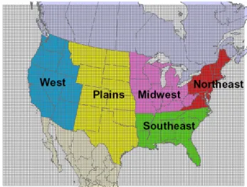
Fig. 1.Simulation domain and US regions.
re-running MM5 with new initial and boundary conditions (i.e.,M (y, x, z, t )INT 0.5%, M (y, x, z, t )INT 50% and
M (y, x, z, t )INT 99.5%from step 2) in order to get
conserva-tive meteorological fields.
We keep the GISS-MM5 field (M (y, x, z, t )GISS−MM5)as the base case scenario in order to compare with current pollu-tant levels (note that new fields of the IGSM 50th percentile climate are not identical to the GISS-MM5 fields). The high-and low-extreme fields are calculated as follows (Eq. 3a high-and b):
High−extreme climate=M (y, x, z, t )99.5%
−M (y, x, z, t )50%+M (y, x, z, t )IGSM−MM5 (3a)
Low−extreme climate=M (y, x, z, t )0.5%
−M (y, x, z, t )50%+M (y, x, z, t )IGSM−MM5 (3b)
It is recognized that using MM5 for downscaling the tem-perature and absolute humidity distributions from the IGSM outputs may not capture the full range of uncertainty in cli-mate change, however, the new fields do capture the extreme cases from the probabilistic distributions of both the meteo-rological fields, and the other meteometeo-rological fields (e.g., pre-cipitation, wind fields, etc.) are dynamically consistent and responsive to the perturbations in temperature and absolute humidity.
2.2 Emission and air quality modeling
MM5 results are inputs to the Sparse Matrix Operating Ker-nel for Emissions (SMOKE) (http://www.smoke-model.org/ index.cfm, last access: 15 December 2008) for estimating emissions of precursors, and to the Community Multiscale Air Quality Model (CMAQ) version 4.3 (Byun and Schere, 2006) for simulating impacts of climate uncertainties on re-gional air quality in 2050. Details of the projections of fu-ture precursor emissions and regional air quality modeling approach are given elsewhere (Tagaris et al., 2007; Woo et al., 2008), and summarized here. The IPCC A1B emission scenario projects decreases in SO2, NOx and non-methane volatile organic compound (NMVOC) emissions from Or-ganization for Economic Co-operation and Development (OECD) countries, including the US and Canada, in 2050s as compared with 1990s based on long-term energy-use and economic trends, which don’t include currently planned pre-cursor emission control regulations (Naki´cenovi´c, 2000). For future regional air quality modeling, projections in regional anthropogenic precursor emission changes are required in addition to national and global emission trends. In this study, projections of regional anthropogenic precursor emis-sions were developed for North America integrating cur-rently planned emission controls (i.e., US Clean Air In-terstate Rule (CAIR); Houyoux, 2004) and long-term eco-nomic and population growth, based on the A1B scenario. Although the same projected emission inventories are ap-plied in the uncertainty simulations in 2050, simulated emis-sions of precursors of pollutants for the three climate sce-narios are not identical since emissions (especially biogenic volatile organic compounds (VOCs)) respond to changes in meteorological fields (e.g., temperature, precipitation, etc.) (see Table S2 http://www.atmos-chem-phys.net/9/865/2009/ acp-9-865-2009-supplement.pdf).
The highest daily maximum 8-h average ozone (MDA8h O3)levels, which are often associated with adverse health effects in epidemiologic studies and used for assessing at-tainment of the US National Ambient Air Quality Stan-dards (NAAQS) for ozone (Bernard et al., 2001; Levy et al., 2001), consistently occur in summer. Three summer months (June, July and August) in the year-2050 are cho-sen as the target period for studying the impact of climate uncertainties on the average and 4th highest MDA8h O3(4th MDA8h O3)concentrations. The 4th highest value is cho-sen as being more stably predicted by chemical transport models than the maximum in any location. For PM2.5, one month from each of the four seasons (i.e., January, April, July and October) in 2050 is chosen for studying the impact of climate uncertainties on annualized PM2.5levels because PM2.5 has distinct seasonal variation and an annual health-based standard (http://www.epa.gov/air/criteria.html, last ac-cess: 15 December 2008). Interannual variability of meteo-rology is a critical issue since only the year 2050 is chosen as the future episode examined in this study. The analysis for the interannual variability of climate fields has been pre-sented by Tagaris et al. (2007): the results show that
cumula-tive distribution function (CDF) and spatial distribution plots for temperature and absolute humidity are similar for the three consecutive future years (2049–2051). The former pa-per provides information on interannual variability, and this paper looks at perturbations to the modeled base meteorol-ogy.
3 Results and discussion
3.1 Meteorology
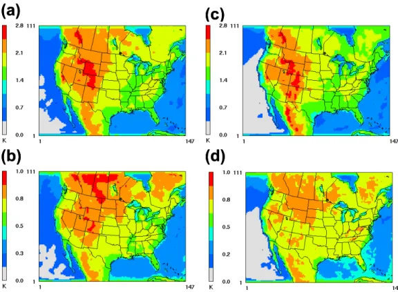
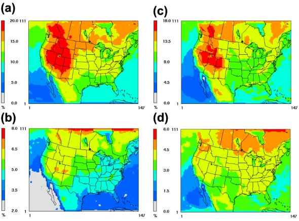
The annualized temperatures (average temperatures of Jan-uary, April, July and October) of the 2050 base GISS-MM5 climate, based on the IPCC A1B scenario, are predicted to be 0.4–2.4 K warmer than 2001, depending on the re-gion, whereas absolute humidity values are simulated to be approximately 0.5 g/Kg (9%)–0.7 g/Kg (14%) higher than 2001 (Table 1). Spatial distributions of annualized temper-ature and absolute humidity between the base case GISS-MM5 and IGSM 50th percentile climate are found to be sim-ilar (Fig. S1 http://www.atmos-chem-phys.net/9/865/2009/ acp-9-865-2009-supplement.pdf), although regional average values differ slightly since the IGSM 50th percentile data has been used for re-running MM5 after being adjusted to the base case GISS-MM5 (Table 1). On the other hand, annualized temperatures and absolute humidity of the two 2050 extreme scenarios are predicted to change approxi-mately from−0.8 K (low-extreme) to+2.1 K (high-extreme) and−0.4 g/Kg (−7%) (low-extreme) to+1.1 g/Kg (+19%) (high-extreme), respectively, as compared with the 2050 base scenario on a regional basis (Table 1). Summer (JJA) tem-peratures and absolute humidity values are predicted to be higher for the 2050 base case than 2001 climate (Table 1). Differences between the high-extreme and base case scenar-ios are found to be larger than differences between the low-extreme and base scenarios for both temperature and abso-lute humidity (Figs. 2 and 3). This reflects that the proba-bility density functions of predicted temperatures and abso-lute humidity are not normally distributed but have a long right-hand tail in the IGSM outputs (Table S1) (Webster et al., 2003). Annualized precipitation is found to be somewhat different for the three scenarios in 2050, with a 0.1 mm/day decrease in summer precipitation in the Plains for the high-extreme scenario as compared with the base case (Fig. 4). The differences in precipitation between the 2050 base case and extreme scenarios are driven by the perturbations in tem-peratures and absolute humidity and based on the extreme percentiles of probabilistic distributions of temperature and absolute humidity changes derived from global modeling in 2050.
3.2 Emissions
Fig. 2.Spatial distribution of difference (K) in temperature in 2050 for(a)annualized (high-extreme – base case);(b)annualized (base case – low-extreme);(c)summer-averaged (high-extreme – base case);(d)summer-averaged (base case – low-extreme) scenarios.
Table 1.Changes in summer-average and annualized temperatures (K), absolute humidity (g/Kg) and total VOC (=anthropogenic+biogenic VOCs) emissions (%) between 2001 and 2050 base case as well as the three 2050 climate scenarios.
Summer-average Annualized
West Plains Midwest Northeast Southeast US West Plains Midwest Northeast Southeast US
Temperature (K)
Base case – 2001 1.8 0.6 0.2 1.8 0.9 1.0 2.4 1.1 1.0 1.8 0.4 1.3
Base case – 50% IGSM Climate 0.5 0.0 −0.5 −0.2 0.3 0.1 0.0 −0.1 −0.1 0.1 0.4 0.0 Low-extreme – Base case −0.7 −0.7 −0.7 −0.7 −0.7 −0.7 −0.7 −0.7 −0.7 −0.6 −0.7 −0.8 High-extreme – Base case 1.9 2.1 1.8 1.7 1.6 1.9 2.1 2.1 1.8 1.7 1.7 1.9
Absolute Humidity (g/Kg)
Base – 2001 0.7 0.6 0.9 0.8 0.5 0.7 0.5 0.5 0.6 0.7 0.7 0.6
Base case – 50% IGSM Climate −2.0 −1.0 −0.2 −0.3 −1.0 −1.0 −0.8 −0.5 −0.1 −0.2 −0.4 −0.5 Low-extreme – Base case −0.3 −0.4 −0.4 −0.4 −0.5 −0.4 −0.3 −0.3 −0.3 −0.4 −0.4 −0.3 High-extreme – Base case 1.0 1.2 1.1 1.1 1.4 1.2 0.8 0.9 0.8 0.8 1.1 0.9
Total VOC Emissions (%)
Base case – 2001 16.6 3.5 −16.9 −3.5 5.3 2.3 11.7 −9.1 −26.3 −19.6 −16.9 −11.8 Low-extreme – Base case −17.0 −10.3 0.4 0.1 −6.9 −8.3 −13.9 −9.1 −1.4 −2.4 −4.9 −7.6 High-extreme – Base case 4.1 14.9 28.5 24.2 15.6 15.4 6.3 14.0 22.0 12.9 17.1 13.2
scenario compared with emissions in 2001, due to planned emission controls. Ammonia (NH3) emissions are simu-lated to increase by about 7% due to increases in popu-lation and related human activities. Total volatile organic compounds (VOC) emissions are predicted to increase by about 2% for the 2050 base case as a net result of
Fig. 3.Spatial distribution of difference (%) in absolute humidity in 2050 for(a)annualized (high-extreme – base case);(b)annualized (base case – low-extreme);(c)summer-averaged (high-extreme – base case);(d)summer-averaged (base case – low-extreme) scenarios.
scenario (Table S2 http://www.atmos-chem-phys.net/9/865/ 2009/acp-9-865-2009-supplement.pdf). However, predicted total VOC emissions vary significantly as biogenic VOC emissions are much more sensitive to temperature changes than other precursor emissions (Tables 1 and S2). Responses of VOC emissions to the extreme climate scenarios are also found to change spatially. The low-extreme scenario results in an approximately 0–17% decrease in total VOC (=anthro-pogenic+biogenic VOC) emissions compared with the 2050 base scenario. For the high-extreme scenario, higher bio-genic VOC emissions cause an increase of up to about 22% in annualized and 29% in summer-average total VOC emis-sions compared with the base case in 2050 on a regional basis (Table 1).
3.3 Summer-average ozone and summertime fourth-highest daily maximum 8-h average ozone
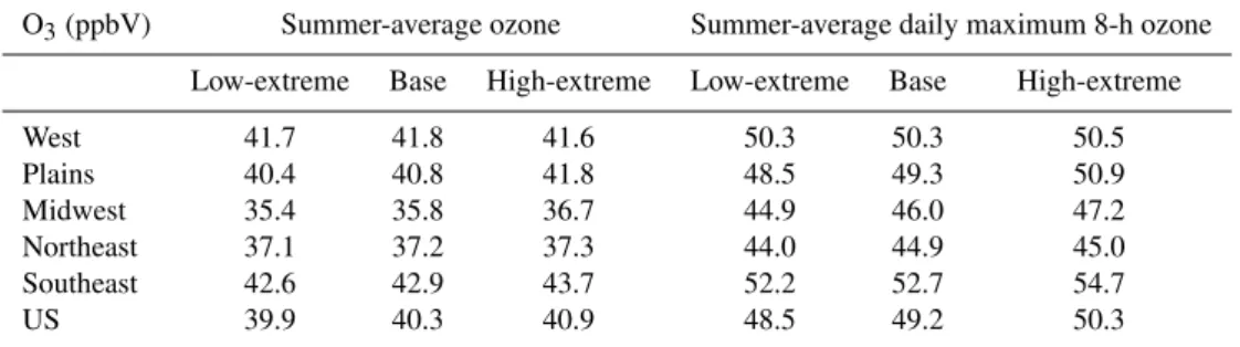
Summer-average ozone and daily maximum 8-h ozone con-centrations are found to be slightly affected by the extreme climate scenarios in 2050 with typical changes of about 1– 2 ppbV between the extreme and base case climate scenar-ios on a regional basis (Table 2). For the peak ozone levels, summertime (JJA) 4th MDA8h O3 (4th MDA8h O3 in the summer of 2050) concentrations for the high-extreme sce-nario are predicted to increase up to 10 ppbV as compared
Fig. 4. Spatial distribution of difference (mm/day) in precipitation in 2050 for(a)annualized (high-extreme – base case);(b)annualized (base – low-extreme);(c)Summer-averaged (high-extreme – base case);(d)summer-averaged (base – low-extreme) scenarios.
Table 2.Summer-average ozone and daily maximum 8-h ozone concentrations (in ppbV) for the three climate scenarios for the five regions and US.
O3(ppbV) Summer-average ozone Summer-average daily maximum 8-h ozone Low-extreme Base High-extreme Low-extreme Base High-extreme
West 41.7 41.8 41.6 50.3 50.3 50.5 Plains 40.4 40.8 41.8 48.5 49.3 50.9 Midwest 35.4 35.8 36.7 44.9 46.0 47.2 Northeast 37.1 37.2 37.3 44.0 44.9 45.0 Southeast 42.6 42.9 43.7 52.2 52.7 54.7 US 39.9 40.3 40.9 48.5 49.2 50.3
VOC emissions (especially biogenic VOC emissions) (Ta-ble 1 and Fig. 6) are considered, higher ozone levels are found in NOx-saturated (or VOC-sensitive) urban areas, e.g., Chicago and New York, and the effects of the high-extreme climate scenario are predicted to be more significant. More-over, for five urban areas in the continental US (i.e., Atlanta, Chicago, Houston, New York and Los Angeles), our previ-ous results show that concentrations of daily maximum 8-h average ozone are predicted to positively respond to VOC emissions on some days for the base case GISS-MM5 sim-ulations in 2050, especially in Chicago and New York,
(a)
(b)
(c)
(d)
g m3 g m3 g m3 g m3
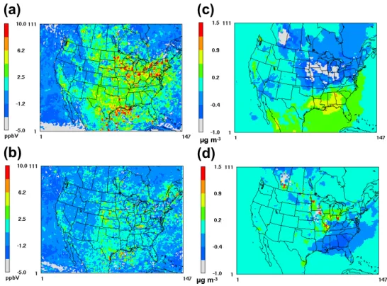
Fig. 5. Spatial distribution of difference in(a)summertime (high-extreme – base scenarios); (b)summertime (base case – low-extreme scenarios) 4th MDA8h O3(ppbV);(c)annualized (high-extreme – base case) PM2.5; and(d)annualized (base case – low-extreme scenario) PM2.5(µg m−3).
and base case climate scenarios does not follow that of tem-perature, absolute humidity and precipitation since ground-level ozone formation is affected by the combined effects of different climate fields and local precursor emissions as well. Differences in concentrations of summertime 4th MDA8h O3are predicted to be approximately+/−3 ppbV between the base case and low-extreme scenarios (Fig. 5). Concen-trations of summertime 4th MDA8h O3are found to be less sensitive to the low-extreme climate scenario than the high-extreme scenario due to smaller differences in meteorolog-ical fields between the base case and low-extreme scenario as well as non-linear responses of ozone concentrations to emission changes (Cohan et al., 2005). Tagaris et al. (2007) present an about 20% decrease in concentrations of summer-average daily maximum 8-h ozone and less number of ex-ceedance days of ozone concentration of 85 ppbV in five US cities between 2000–2002 and 2049–2051, mainly due to currently planned emission controls in the future. Here, a maximum change of 10 ppbV in 4th MDA8h O3(about one-seventh of the current NAAQS of ozone of 75 ppbV) is found in 2050 for the high-extreme climate scenario, which may significantly offset the effectiveness of currently planned emission reductions in urban areas with high concentrations of PANs, VOC, CH4and CO as well as VOC-sensitive ozone formation regimes.
3.4 Annualized PM2.5
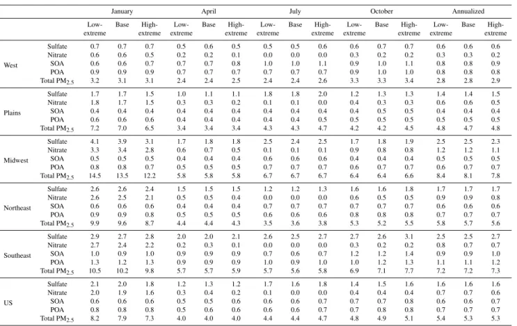
Table 3.Annualized and seasonal (January, April, July and October) total PM2.5levels and composition (sulfate, nitrate, secondary organic aerosol (SOA) and primary organic aerosol (POA)) for the three climate scenarios in 2050 for the five regions and US Unit:µg m−3.
January April July October Annualized
Low- Base High- Low- Base High- Low- Base High- Low- Base High- Low- Base High-extreme extreme extreme extreme extreme extreme extreme extreme extreme extreme
West
Sulfate 0.7 0.7 0.7 0.5 0.6 0.5 0.5 0.5 0.6 0.6 0.7 0.7 0.6 0.6 0.6 Nitrate 0.6 0.6 0.5 0.2 0.2 0.1 0.0 0.0 0.0 0.3 0.2 0.2 0.3 0.3 0.2
SOA 0.6 0.6 0.7 0.7 0.7 0.8 1.0 1.0 1.1 0.9 1.0 1.1 0.8 0.8 0.9
POA 0.9 0.9 0.9 0.7 0.7 0.7 0.7 0.7 0.7 0.9 1.0 1.0 0.8 0.8 0.8
Total PM2.5 3.2 3.1 3.1 2.4 2.4 2.5 2.4 2.4 2.6 3.3 3.3 3.4 2.8 2.8 2.9
Plains
Sulfate 1.7 1.7 1.5 1.0 1.1 1.1 1.8 1.8 2.0 1.2 1.3 1.3 1.4 1.4 1.5 Nitrate 1.8 1.7 1.5 0.3 0.3 0.2 0.1 0.1 0.0 0.4 0.3 0.3 0.6 0.6 0.5
SOA 0.4 0.4 0.4 0.4 0.4 0.4 0.4 0.4 0.4 0.4 0.5 0.5 0.4 0.4 0.4
POA 0.6 0.6 0.6 0.4 0.4 0.4 0.4 0.4 0.5 0.5 0.5 0.5 0.5 0.5 0.5
Total PM2.5 7.2 7.0 6.5 3.4 3.4 3.4 4.3 4.3 4.7 4.2 4.2 4.5 4.8 4.7 4.8
Midwest
Sulfate 4.1 3.9 3.1 1.7 1.8 1.8 2.5 2.4 2.5 1.7 1.8 1.9 2.5 2.5 2.3 Nitrate 3.3 3.4 2.8 0.6 0.7 0.5 0.1 0.1 0.1 0.9 0.8 0.8 1.2 1.2 1.1
SOA 0.5 0.5 0.5 0.4 0.4 0.4 0.6 0.6 0.6 0.4 0.4 0.4 0.5 0.5 0.5
POA 0.8 0.8 0.7 0.5 0.5 0.5 0.7 0.7 0.7 0.6 0.7 0.7 0.6 0.7 0.7
Total PM2.5 14.5 13.5 12.2 5.8 5.8 5.8 6.7 6.7 6.7 6.4 6.4 6.6 8.4 8.1 7.8
Northeast
Sulfate 2.6 2.6 2.4 1.5 1.5 1.5 1.2 1.2 1.3 1.6 1.6 1.8 1.7 1.7 1.7 Nitrate 2.6 2.5 2.1 0.5 0.5 0.4 0.0 0.0 0.0 0.6 0.5 0.5 0.9 0.9 0.8
SOA 0.6 0.6 0.6 0.4 0.4 0.4 0.7 0.7 0.7 0.7 0.7 0.7 0.6 0.6 0.6
POA 0.9 0.9 0.8 0.5 0.5 0.5 0.6 0.6 0.6 0.8 0.8 0.8 0.7 0.7 0.7
Total PM2.5 9.9 9.6 8.7 4.4 4.4 4.3 3.5 3.6 3.8 5.3 5.2 5.5 5.8 5.7 5.6
Southeast
Sulfate 2.9 2.7 2.8 2.0 2.0 2.1 2.6 2.5 2.7 2.7 2.6 3.1 2.5 2.5 2.7 Nitrate 2.7 2.4 2.2 0.2 0.3 0.1 0.0 0.0 0.0 0.3 0.2 0.2 0.8 0.7 0.7
SOA 1.0 0.9 1.0 0.9 0.9 0.9 0.7 0.6 0.7 1.2 1.2 1.4 0.9 0.9 1.0
POA 1.3 1.2 1.3 0.9 0.9 0.9 1.0 0.9 1.0 1.0 1.2 1.3 1.1 1.1 1.2
Total PM2.5 10.5 10.2 9.8 5.7 5.7 5.9 5.7 5.6 5.8 6.9 7.1 7.7 7.2 7.2 7.3
US
Sulfate 2.1 2.0 1.8 1.2 1.3 1.2 1.7 1.6 1.8 1.4 1.5 1.6 1.6 1.6 1.6 Nitrate 2.0 1.9 1.6 0.3 0.4 0.2 0.1 0.0 0.0 0.4 0.4 0.4 0.7 0.7 0.6
SOA 0.6 0.6 0.6 0.5 0.5 0.6 0.6 0.6 0.7 0.7 0.7 0.8 0.6 0.6 0.7
POA 0.8 0.8 0.8 0.5 0.6 0.6 0.6 0.6 0.7 0.7 0.8 0.8 0.7 0.7 0.7
Total PM2.5 8.2 7.9 7.3 4.0 4.0 4.0 4.4 4.4 4.7 4.8 4.9 5.1 5.4 5.3 5.3
increase in annualized PM2.5levels in the Southeast for the low-extreme scenario is due to higher nitrate in the winter (January) than the base case (Table 3). SOA is predicted to be influenced by changes in biogenic VOC emissions as well as modifications in the formation rates under the effects of the extreme climate scenarios. In CMAQ version 4.3, the SOA gas-particle partitioning model is based on the Sec-ondary Organic Aerosol Model (SORGAM) (Schell et al., 2001), which doesn’t account for SOA formation from iso-prene. Some studies show that isoprene significantly con-tributes to SOA formation (Claeys et al., 2004), and SOA levels are predicted to be underestimated without including isoprene as a SOA precursor (Zhang et al., 2007; Morris et al., 2006; Pun and Seigneur, 2007). In this study, the changes in PM2.5levels attributed to the extreme climate scenarios are dominated by sulfate and nitrate PM2.5in most of the US re-gions since SOA formation is not fully captured in current regional air quality models (Table 3).
Impacts of climate uncertainties on PM2.5concentrations also show a seasonal trend. Monthly-average PM2.5 con-centrations are predicted to be lower in January but slightly higher in July for the high-extreme scenario compared with the 2050 base case (Table 3); this is mainly because
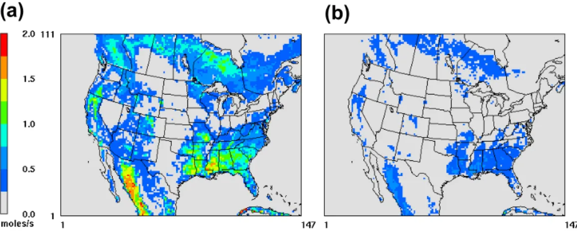
Fig. 6.Spatial distribution of difference (moles/s) in summertime biogenic VOC emissions between(a)high-extreme and base case as well as(b)base case – low-extreme scenarios.
statistical analysis, PM is not as weather-dependent as ozone in the southwestern US since low precipitation is found in the studying region. The results in this study also show that an-nualized PM2.5levels are not as sensitive as concentrations of summertime peak ozone with respect to the extreme climate scenarios examined since one of the main removal mecha-nisms of PM2.5, precipitation scavenging, is found to slightly affect annualized PM2.5levels between the extreme climate scenarios (Fig. 4). Our previous study shows that annual av-erage PM2.5levels are predicted to decrease by about 23% (regionally varies from−9% to−32%) in 2050 as a com-bined effect of future climate change and CAIR emission controls (Tagaris et al., 2007). The results here imply that, on a regional basis, future emission controls will still be ef-fective in decreasing annualized PM2.5levels with respect to the extreme climate scenarios if precipitation is only slightly affected.
4 Response of air quality to emission controls under ex-treme climate scenarios
In addition to simulating how the alternative extreme scenar-ios impact pollutant levels, we also investigate the responses of ozone and PM2.5levels to emission controls under the ex-treme climate scenarios. CMAQ, with the Decoupled Direct Method-3D (DDM-3D) (Dunker et al., 2002; Yang et al., 1997), is used to quantify sensitivities of ozone and PM2.5 to precursor emissions. First-order sensitivities (Si,j)of pol-lutant concentrationi(Ci)(i.e. ozone and PM2.5)to source emissions j (Ej) (i.e., anthropogenic VOC, anthropogenic NOx and total SO2 emissions) are defined as (Yang et al., 1997):
Si,j =Ej
∂Ci
∂Ej
(4b)
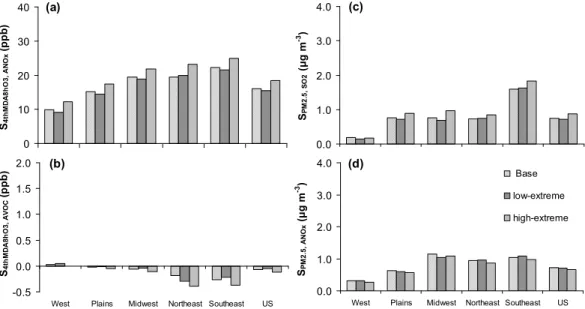
First-order sensitivities represent the locally linear responses of pollutant concentrations to emission changes and have the same units as the concentrations. Sensitivities of sum-mertime 4th MDA8h O3 to anthropogenic NOx emissions (S4th MDA8h O3,A NOx) are predicted to slightly decrease for
the low-extreme scenario but increase for the high-extreme scenario as compared with the base case in 2050. The dif-ferences are mainly attributed to the climate effects on bio-genic VOC emissions and photochemistry. Biobio-genic VOC emissions are predicted to increase for the high-extreme sce-nario, especially in the Southeast region and west coast of the continental US, compared with the base case in the sum-mer of 2050 (Fig. 6). Higher biogenic VOC emissions for the high-extreme attribute to a more NOx-limit environment for ozone formation and increase S4th MDA8h O3,A NOx. The
effects of the extreme climate scenarios on sensitivities of summertime 4th MDA8h O3 to anthropogenic VOC emis-sions (S4th MDA8h O3,A VOC)are predicted to be small (Fig. 7).
For the responses of PM2.5to emission changes under the ex-treme climate scenarios, sensitivities of annualized PM2.5to SO2emissions (SPM2.5,SO2)are predicted to slightly increase
for the high-extreme scenario on a regional basis, because of higher temperature, humidity, decreased rainfall in some re-gions, and faster oxidation of precursors as compared with the base scenario. Higher temperatures for the high-extreme scenario favor particulate NH4NO3 to dissociate to its gas phase precursors and cause slight decreases in sensitivities of annualized PM2.5 concentrations to anthropogenic NOx emissions (SPM2.5,A NOx)(Fig. 7). Overall, on a regional
ba-sis, the effectiveness of NOxand SO2emission controls for reducing peak ozone and PM2.5levels changes little, though climate-driven increases in extreme ozone levels may require additional controls to reach applicable air quality standards.
Fig. 7.Sensitivities of 4th MDA8h O3to(a)anthropogenic NOx(S4th MDA8h O3,A NOx)and(b)anthropogenic VOC (S4th MDA8h O3,A VOC)
(ppbV) as well as sensitivities of annualized PM2.5 to(c)anthropogenic SO2 (SPM2.5,SO2)and (d)anthropogenic NOx (SPM2.5,A NOx)
(µg m−3)in 2001 and the 2050 base and extreme scenarios for the five regions and US.
Table 4.Annualized monthly maximum daily PM2.5levels (average of monthly maximum daily PM2.5for January, April, July and October) and their sensitivities to SO2(SPM2.5,SO2), anthropogenic NOx(SPM2.5,A NOx)and VOC (SPM2.5,A VOC)for the five US cities for the three
climate scenarios in 2050 Unit:µg m−3.
2050 Low-extreme 2050 Base 2050 High-extreme
Los Angeles
PM2.5 21.9 22.1 24.2
SPM2.5,SO2 0.0 0.1 0.0
SPM2.5,A NOx 0.3 0.9 0.4
SPM2.5,A VOC 0.5 0.5 0.6
Houston
PM2.5 25.1 25.2 24.6
SPM2.5,SO2 3.0 3.3 3.9
SPM2.5,A NOx 3.3 3.1 2.6
SPM2.5,A VOC −0.1 −0.1 −0.1
Chicago
PM2.5 36.5 36.9 38.3
SPM2.5,SO2 1.7 1.9 3.3
SPM2.5,A NOx 5.2 4.7 7.3
SPM2.5,A VOC 0.7 0.7 0.4
New York
PM2.5 35.7 34.9 36.5
SPM2.5,SO2 1.7 1.5 1.5
SPM2.5,A NOx 3.3 3.0 1.7
SPM2.5,A VOC 0.9 0.9 1.0
Atlanta
PM2.5 26.5 26.4 27.1
SPM2.5,SO2 2.6 2.6 2.5
SPM2.5,A NOx 2.0 1.9 2.8
in 2050 for five US urban areas, Atlanta, Chicago, Houston, Los Angeles and New York, where currently have high PM2.5 levels (http://www.epa.gov/oar/oaqps/greenbk/, last access: 15 December 2008). Such areas are particularly susceptible to the climate penalty, especially when tightening of future daily average PM2.5 standards is considered. For the five cities examined, sensitivities of annualized monthly maxi-mum daily PM2.5to anthropogenic NOxemissions are pre-dicted to be affected by the extreme climate scenarios, with changes up to 2.6µg m−3 (Table 4), since ammonium ni-trate (NH4NO3)formation is very responsive to changes in meteorology (particularly temperature, Stelson and Seinfeld, 1982). Responses of annualized monthly maximum daily PM2.5 to SO2 emissions are also predicted to be different under the extreme climate scenarios in Chicago due to high SO2 emissions in the Midwest region of the US (Table 4). For four of the five cities examined, Los Angeles being the exception, reductions in SO2and anthropogenic NOx emis-sions are predicted to continue to be still effective for de-creasing annualized monthly peak daily PM2.5levels under the extreme climate scenarios in 2050. While reductions in anthropogenic NOxand VOCs emissions are predicted to be effective for decreasing annualized monthly peak PM2.5 lev-els in Los Angeles for the three climate scenarios in 2050. Overall, the results for the five cities show that, although the effectiveness of emission controls for decreasing peak PM2.5 levels responds to the extreme climate scenarios, the direc-tions of currently planned emission controls will not be sig-nificantly affected.
5 Conclusions
Uncertainties associated with simulations of the extreme cli-mate scenarios are found to have a rather moderate effect on predicted emissions of VOC and concentrations of fourth-highest daily maximum 8-h average ozone in year 2050. Differences in concentrations of fourth-highest daily maxi-mum 8-h average ozone between the extreme climate sce-narios and base case are found up to 10 ppbV (about one-seventh of the current ozone standards of 75 ppbV) in some polluted urban areas due to the combined effects of higher temperature, absolute humidity and VOC emissions, though the change in summer-average ozone is minimal on a re-gional basis (∼1 ppbV). Differences between the extreme and base scenarios in annualized PM2.5levels are predicted to range between−1.0 and+1.5µg m−3. For the five US cities examined, sensitivities of annualized monthly maxi-mum daily PM2.5to anthropogenic NOxemissions are pre-dicted to influenced by the extreme climate scenarios since temperature changes significantly affect ammonium nitrate (NH4NO3) formation. Responses of annualized monthly maximum daily PM2.5 to SO2 emissions change most in the Midwest due to locally high emissions. Overall, fu-ture annualized PM2.5is predicted to be less sensitive to the
extreme climate scenarios than summertime fourth-highest daily maximum 8-h average ozone since precipitation scav-enging is not significantly changed with the extreme climate scenarios where perturbations in temperatures and absolute humidity from the global model are used to drive changes in the regional meteorological modeling. Planned controls for decreasing regional ozone and PM2.5will continue to be effective in the future under the extreme climate scenarios. However, the impact of climate uncertainties may be substan-tial in some urban areas and should be included in assessing future regional air quality and emission control requirements.
Acknowledgements. The authors would like to thank US Environ-mental Protection Agency for providing funding for this project under Science To Achieve Results (STAR) grant No. RD83096001, RD82897602 and RD83107601 and Eastern Tennessee State University. The views expressed in this paper are those of the authors and do not necessarily reflect the views or policies of the EPA. The authors would also like to thank L. Ruby Leung from Pacific Northwest National Laboratory for providing future meteorological data and Loretta Mickley from Harvard University for the GISS simulation used by Leung and Marcus Sarofim for his help in collecting the needed IGSM data.
Edited by: J. Rinne
References
Aw, J. and Kleeman, M. J.: Evaluating the first-order ef-fect of intraannual temperature variability on urban air pollution, J. Geophys. Res.-Atmos., 108(D12), 4365, doi:10.1029/2002JD002688, 2003.
Babiker, M., Reilly, J., and Ellerman, D.: Japanese nuclear power and the kyoto agreement, J. Jpn. Int. Econ., 14, 169–188, 2000. Baertsch-Ritter, N., Keller, J., Dommen, J., and Prevot, A. S. H.:
Effects of various meteorological conditions and spatial emis-sionresolutions on the ozone concentration and ROG/NOx lim-itationin the Milan area (I), Atmos. Chem. Phys., 4, 423–438, 2004,
http://www.atmos-chem-phys.net/4/423/2004/.
Bergin, M. S., Russell, A. G., and Milford, J. B.: Effects of chem-ical mechanism uncertainties on the reactivity quantification of volatile organic compounds using a three-dimensional air qual-ity model, Environ. Sci. Technol., 32, 694–703, 1998.
Bernard, S. M., Samet, J. M., Grambsch, A., Ebi, K. L., and Romieu, I.: The potential impacts of climate variability and change on air pollution-related health effects in the united states, Environ. Health Persp., 109, 199–209, 2001.
Byun, D. W. and Schere, K. L.: Review of the governing equations, computational algorithms, and other components of the models-3 community multscale air quality (cmaq) modeling system, Appl. Mech. Rev., 59, 51–77, 2006.
Cohan, D. S., Hakami, A., Hu, Y. T., and Russell, A. G.: Nonlinear response of ozone to emissions: Source apportionment and sen-sitivity analysis, Environ. Sci. Technol., 39, 6739–6748, 2005. Dawson, J. P., Adams, P. J., and Pandis, S. N.: Sensitivity of ozone
to summertime climate in the eastern USA: A modeling case study, Atmos. Environ., 41, 1494–1511, 2007.
Dunker, A. M., Yarwood, G., Ortmann, J. P., and Wilson, G. M.: The decoupled direct method for sensitivity analysis in a three-dimensional air quality model – implementation, accuracy, and efficiency, Environ. Sci. Technol., 36, 2965–2976, 2002. Galizia, A. and Kinney, P. L.: Long-term residence in areas of high
ozone: Associations with respiratory health in a nationwide sam-ple of nonsmoking young adults, Environ. Health Persp., 107, 675–679, 1999.
Grell, G., Dudhia, J., and Stauffer, D. R.: A description of the fifth generation penn state/ncar mesoscale model (mm5) – ncar tech. Note – ncar/tn-398+str, Natl. Cent for Atmos. Res., Boulder, Col-orado, 1994.
Gustafson, W. I. and Leung, L. R.: Regional downscaling for air quality assessment – a reasonable proposition?, B. Am. Meteo-rol. Soc., 88, 1215–1227, 2007.
Hanna, S. R., Lu, Z. G., Frey, H. C., Wheeler, N., Vukovich, J., Arunachalam, S., Fernau, M., and Hansen, D. A.: Uncertainties in predicted ozone concentrations due to input uncertainties for the uam-v photochemical grid model applied to the july 1995 otag domain, Atmos. Environ., 35, 891–903, 2001.
Hanna, S. R., Russell, A. G., Wilkinson, J. G., Vukovich, J., and Hansen, D. A.: Monte carlo estimation of uncertainties in beis3 emission outputs and their effects on uncertainties in chemi-cal transport model predictions, J. Geophys. Res.-Atmos., 110, D01302, doi:10.1029/2004JD004986, 2005.
Hogrefe, C., Lynn, B., Civerolo, K., Ku, J. Y., Rosenthal, J., Rosen-zweig, C., Goldberg, R., Gaffin, S., Knowlton, K., and Kin-ney, P. L.: Simulating changes in regional air pollution over the eastern united states due to changes in global and regional climate and emissions, J. Geophys. Res.-Atmos., 109, D22301. doi:10.1029/2004JD004690, 2004.
Holian, G., Sokolov, A., and Prinn, R.: Uncertainty in atmospheric CO2 predictions from a parametric uncertainty analysis of a global ocean carbon cycle model, report no. 80, Joint Program on the Science and Policy of Global Change, MIT, Boston, MA, 2001.
Houyoux, M.: Cair emissions inventory overview, US Environmen-tal Protection Agency, 2004.
IPCC: Climate change 2007: The physical science basis, Cam-bridge University Press, CamCam-bridge, UK, 2007.
Johnson, P. R. S. and Graham, J. J.: Fine particulate matter national ambient air quality standards: Public health impact on popula-tions in the northeastern united states, Environ. Health Persp., 113, 1140–1147, 2005.
Leung, L. R. and Gustafson, W. I.: Potential regional climate change and implications to us air quality, Geophys. Res. Lett., 32, L16711, doi:10.1029/2005GL022911, 2005.
Levy, J. I., Carrothers, T. J., Tuomisto, J. T., Hammitt, J. K., and Evans, J. S.: Assessing the public health benefits of reduced ozone concentrations, Environ. Health Persp., 109, 1215–1226, 2001.
Liao, K. J., Tagaris, E., Manomaiphiboon, k., Woo, J. H., He, S., Amar, P., and Russell, A. G.: Current and future linked responses
of ozone and PM2.5to emission controls, Environ. Sci. Technol., 42, 4670–4675, 2008.
Melillo, J. M., McGuire, A. D., Kicklighter, D. W., Moore, B., Vorosmarty, C. J., and Schloss, A. L.: Global climate-change and terrestrial net primary production, Nature, 363, 234–240, 1993. Menut, L.: Adjoint modeling for atmospheric pollution process
sen-sitivity at regional scale, J. Geophys. Res.-Atmos., 108(D17), 8562, doi:10.1029/2002JD002549, 2003.
Mickley, L. J., Jacob, D. J., Field, B. D., and Rind, D.: Effects of future climate change on regional air pollution episodes in the united states, Geophys. Res. Lett., 31, L24103, doi:10.1029/2004GL021216, 2004.
Morris, R. E., Koo, B., Guenther, A., Yarwood, G., McNally, D., Tesche, T. W., Tonnesen, G., Boylan, J., and Brewer, P.: Model sensitivity evaluation for organic carbon using two multi-pollutant air quality models that simulate regional haze in the southeastern united states, Atmos. Environ., 40, 4960–4972, 2006.
Murazaki, K. and Hess, P.: How does climate change contribute to surface ozone change over the united states?, J. Geophys. Res.-Atmos., 111, D05301, doi:10.1029/2005JD005873, 2006. Naki´cenovi´c, N.: Special report on emissions scenarios, Cambridge
University Press, Cambridge, UK, 2000.
Nenes, A., Pandis, S. N., and Pilinis, C.: Isorropia: A new ther-modynamic equilibrium model for multiphase multicomponent inorganic aerosols, Aquat. Geochem., 4, 123–152, 1998. Prinn, R., Jacoby, H., Sokolov, A., Wang, C., Xiao, X., Yang, Z.,
Eckhaus, R., Stone, P., Ellerman, D., Melillo, J., Fitzmaurice, J., Kicklighter, D., Holian, G., and Liu, Y.: Integrated global system model for climate policy assessment: Feedbacks and sensitivity studies, Clim. Change, 41, 469–546, 1999.
Pun, B. K. and Seigneur, C.: Investigative modeling of new path-ways for secondary organic aerosol formation, Atmos. Chem. Phys., 7, 2199–2216, 2007,
http://www.atmos-chem-phys.net/7/2199/2007/.
Racherla, P. N. and Adams, P. J.: Sensitivity of global tro-pospheric ozone and fine particulate matter concentrations to climate change, J. Geophys. Res.-Atmos., 111, D24103, doi:10.1029/2005JD006939, 2006.
Rae, J. G. L., Johnson, C. E., Bellouin, N., Boucher, O., Haywood, J. M., and Jones, A.: Sensitivity of global sulphate aerosol pro-duction to changes in oxidant concentrations and climate, J. Geo-phys. Res.-Atmos., 112, D10312, doi:10.1029/2006JD007826, 2007.
Reilly, J., Prinn, R., Harnisch, J., Fitzmaurice, J., Jacoby, H., Kick-lighter, D., Melillo, J., Stone, P., Sokolov, A., and Wang, C.: Multi-gas assessment of the kyoto protocol, Nature, 401, 549– 555, 1999.
Rind, D., Lerner, J., Shah, K., and Suozzo, R.: Use of on-line trac-ers as a diagnostic tool in general circulation model development 2. Transport between the troposphere and stratosphere, J. Geo-phys. Res.-Atmos., 104, 9151–9167, 1999.
Russell, A. and Dennis, R.: Narsto critical review of photochemical models and modeling, Atmos. Environ., 34, 2283–2324, 2000. Sanderson, M. G., Jones, C. D., Collins, W. J., Johnson, C. E., and
Derwent, R. G.: Effect of climate change on isoprene emissions and surface ozone levels, Geophys. Res. Lett., 30(18), 1936, doi:10.1029/2003GL017642, 2003.
A.: Modeling the formation of secondary organic aerosol within a comprehensive air quality model system, J. Geophys. Res.-Atmos., 106, 28275–28293, 2001.
Seaman, N. L.: Meteorological modeling for air-quality assess-ments, Atmos. Environ., 34, 2231–2259, 2000.
Seinfeld, J. H. and Pandis, S. N.: Atmospheric chemistry and physics: From air pollution to climate change, 2nd ed., John Wi-ley & Sons, Inc., New York, 2006.
Sillman, S. and Samson, F. J.: Impact of temperature on oxi-dant photochemistry in urban, polluted rural and remote envi-ronments, J. Geophys. Res.-Atmos., 100, 11497–11508, 1995. Sokolov, A. P. and Stone, P. H.: A flexible climate model for use in
integrated assessments, Clim. Dynam., 14, 291–303, 1998. Stelson, A. W. and Seinfeld, J. H.: Thermodynamic prediction of
the water activity, NH4NO3 dissociation-constant, density and refractive-index for the NH4NO3-(NH4)2SO4-H2O system at 25-degrees-C, Atmos. Environ., 16, 2507–2514, 1982.
Strader, R., Lurmann, F., and Pandis, S. N.: Evaluation of secondary organic aerosol formation in winter, Atmos. Environ., 33, 4849– 4863, 1999.
Tagaris, E., Manomaiphiboon, K., Liao, K. J., Leung, L. R., Woo, J. H., He, S., Amar, P., and Russell, A. G.: Impacts of global climate change and emissions on regional ozone and fine partic-ulate matter concentrations overthe us, J. Geophys. Res.-Atmos., 112, D14312, doi:10.1029/2006JD008262, 2007.
Tian, H., Melillo, J. M., Kicklighter, D. W., McGuire, A. D., and Helfrich, J.: The sensitivity of terrestrial carbon storage to histor-ical climate variability and atmospheric CO2in the united states, Tellus Series B-Chemical and Physical Meteorology, 51, 414– 452, 1999.
Wang, C., Prinn, R. G., and Sokolov, A.: A global interactive chem-istry and climate model: Formulation and testing, J. Geophys. Res.-Atmos., 103, 3399–3417, 1998.
Webster, M., Forest, C., Reilly, J., Babiker, M., Kicklighter, D., Mayer, M., Prinn, R., Sarofim, M., Sokolov, A., Stone, P., and Wang, C.: Uncertainty analysis of climate change and policy re-sponse, Clim. Change, 61, 295–320, 2003.
Wise, E. K. and Comrie, A. C.: Meteorologically adjusted urban air quality trends in the southwestern united states, Atmos. Environ., 39, 2969–2980, 2005.
Woo, J. H., He, S. P., Amar, P., Tagaris, E., Manomaiphiboon, K., Liao, K. J., and Russell, A. G.: Development of mid-century an-thropogenic emissions inventory in support of regional air quality modeling under influence of climate change, J. Air Waste Mag. Asso., 58, 1483–1494, 2008.
Wunderli, S. and Gehrig, R.: Influence of temperature on formation and stability of surface pan and ozone – a 2-year field-study in switzerland, Atmos. Environ., Part a-General Topics, 25, 1599– 1608, 1991.
Yang, Y. J., Wilkinson, J. G., and Russell, A. G.: Fast, direct sensi-tivity analysis of multidimensional photochemical models, Env-iron. Sci. Technol., 31, 2859–2868, 1997.