www.atmos-meas-tech.net/8/2017/2015/ doi:10.5194/amt-8-2017-2015
© Author(s) 2015. CC Attribution 3.0 License.
Measurements of methane emissions from natural gas gathering
facilities and processing plants: measurement methods
J. R. Roscioli1, T. I. Yacovitch1, C. Floerchinger1, A. L. Mitchell2, D. S. Tkacik2, R. Subramanian2, D. M. Martinez3, T. L. Vaughn3, L. Williams5, D. Zimmerle4, A. L. Robinson2, S. C. Herndon1, and A. J. Marchese3
1Aerodyne Research Inc., Billerica, MA, USA
2Department of Mechanical Engineering, Carnegie Mellon University, Pittsburgh, PA 15213, USA 3Department of Mechanical Engineering, Colorado State University, Fort Collins, CO 80523, USA 4The Energy Institute, Colorado State University, Fort Collins, CO 80523, USA
5Fort Lewis College, Durango, CO 81301, USA
Correspondence to:S. C. Herndon ([email protected])
Received: 29 October 2014 – Published in Atmos. Meas. Tech. Discuss.: 11 December 2014 Revised: 31 March 2015 – Accepted: 10 April 2015 – Published: 7 May 2015
Abstract. Increased natural gas production in recent years has spurred intense interest in methane (CH4)emissions
as-sociated with its production, gathering, processing, trans-mission, and distribution. Gathering and processing facili-ties (G&P facilifacili-ties) are unique in that the wide range of gas sources (shale, coal-bed, tight gas, conventional, etc.) sults in a wide range of gas compositions, which in turn re-quires an array of technologies to prepare the gas for pipeline transmission and distribution. We present an overview and detailed description of the measurement method and analy-sis approach used during a 20-week field campaign studying CH4emissions from the natural gas G&P facilities between
October 2013 and April 2014. Dual-tracer flux measure-ments and on-site observations were used to address the mag-nitude and origins of CH4 emissions from these facilities.
The use of a second tracer as an internal standard revealed plume-specific uncertainties in the measured emission rates of 20–47 %, depending upon plume classification. Combin-ing downwind methane, ethane (C2H6), carbon monoxide
(CO), carbon dioxide (CO2), and tracer gas measurements
with on-site tracer gas release allows for quantification of fa-cility emissions and in some cases a more detailed picture of source locations.
1 Introduction
The natural gas industry has undergone a transformation in recent years, largely due to technological advancements such as hydraulic fracturing and horizontal drilling. These ad-vances have led to increases in domestic natural gas produc-tion (EPA, 2014b), although concomitant with this increase has been a rising concern over methane emissions from the entire natural gas system from the perspective of both envi-ronmental impact and a loss of resources or product. Over the past decade, many studies have aimed at quantifying these emissions using a variety of methods, yielding a wide range of methane loss rate assessments for various sectors and basins from < 0.5 % to greater than 10 % (Pétron et al., 2012a and b; Allen et al., 2013; Karion et al., 2013; Bullock and Nettles, 2014; Subramanian et al., 2014; Zimmerle et al., 2014; Harrison et al., 2011; Zavala-Araiza et al., 2014).
The path of natural gas from well to the consumer can be considered in terms of five possible steps: production, gath-ering, processing, transmission and storage, and distribution. A recent series of studies have investigated CH4emissions
production, transmission, and storage facilities (Allen et al., 2013; Subramanian et al., 2014; Lamb et al., 2015). Of par-ticular emphasis in this report are the measurement approach to the field campaign and the unique emission profiles as-sociated with gathering and processing, illustrating the wide variety of handling, treating, and processing tools at the dis-posal of the natural gas industry. The G&P field campaign was executed by Aerodyne Research, Inc. (ARI), Carnegie Mellon University (CMU), and Colorado State University from October 2013 through April 2014. Mobile laboratories operated by ARI and CMU sampled emissions from a to-tal of 130 G&P facilities across 20 natural gas basins in 13 states, using tracer release methodology as discussed below. The measurements were performed with cooperation from industry partners, who provided site access and detailed fa-cility data, such as natural gas throughput, gas type, gas com-position, equipment inventories, compressor power, age, and inlet/outlet pressures. Efforts were made by the study partici-pants to ensure that the facilities were sampled as found, and the resulting data were assigned random numbers such that they cannot be traced back to a specific facility or partner company.
The inherent chemical profile of natural gas from different sources can significantly affect the technological approach that G&P facilities use to prepare the gas for delivery into the transmission pipeline system. In order to sample from the wide range of equipment employed during gathering and processing, the campaign measured emissions from facilities associated with a variety of types of gas, such as gas with low- and high-C2+hydrocarbon content (here referred to as
dry and wet gas, respectively), as well as sour (high sulfur and/or CO2content) and sweet gas sources (low sulfur and/or
CO2content). More detailed information about site selection
is presented by Mitchell et al. in the companion paper, “Mea-surement Results” (Mitchell et al., 2015). These facilities handled natural gas derived from a variety of origins, includ-ing shale, coal-bed, and conventional wells. In many cases, the emission profiles associated with these facilities reflect the equipment used to prepare the natural gas (EIA, 2006; Kidnay et al., 2011). For example, the first step during gath-ering is often passage through gathgath-ering lines and a compres-sor (gathering) station. One of the primary purposes of gath-ering facilities is to collect and compress the input stream of gas to pipeline pressures, usually ∼800 psi (∼55 bar). This requires the use of compressors and associated equip-ment, for which there are multiple possible emission sources such as compressor seals, natural-gas-driven pneumatic de-vices, and engine exhaust. Frequently gathering facilities will also remove water from the gas stream using dehydration trains, which provide more possible emissions points. Fol-lowing gathering, sweet, dry gas can typically be easily con-ditioned and sent to the distribution network. However, gas that is sour, wet, or with a high water content requires signif-icant subsequent processing, such as the removal of natural gas liquids (NGLs) using forced extraction, and sometimes
a dehydration step to further remove water (Kidnay et al., 2011; Jumonville, 2010). These relatively complex structures can involve distillation columns, turboexpanders, separators, compressors, pneumatic devices, and heat exchangers, all of which can emit CH4 either through minor fugitive
compo-nents or venting. Finally, extracted natural gas can have high CO2 and/or H2S content (i.e., sour, especially in coal-bed
methane and some shale-gas regions), which requires amine treating (frequently collocated with other gas processing or compression facilities) to make it distribution-ready (Kidnay et al., 2011). Again, this equipment and additional processing adds to the number of possible emission sources.
Presented in the second half of this paper are examples of the unique chemical profiles associated with the gather-ing, treatment, and processing systems utilized by the nat-ural gas industry. In the process of measuring CH4
emis-sion rates, these signatures can provide important informa-tion about contribuinforma-tions from specific methane sources on site.
2 Challenges in measuring emissions from natural gas facilities
The necessity for emissions measurements at natural gas fa-cilities is two-fold: (i) as an assessment of the impact of facil-ity operation upon regional and national air qualfacil-ity and cli-mate (EPA, 2014a) and (ii) to quantify losses due to normal operation or identify large emission sources. In the case of (i), measured emissions provide an opportunity to compare to national estimates and assess the overall impact of the nat-ural gas supply chain on CH4emissions in the US.
(March-ese et al., 2015; Subramanian et al., 2014). In the case of (ii), these measurements aid the natural gas industry in minimiz-ing product losses.
2.1 Bottom-up approaches
plants, where the inability to measure emissions from a large number of components could lead to an asymmetric bias in the reported FLER. In addition, in order to accurately scale bottom-up studies to nationwide (or even regional) estimates, care must be taken to ensure that the sampled population, which is typically small, accurately represents the national or regional inventory of facilities.
Optical gas imaging (e.g., infrared cameras such as FLIR®) is a method by which leaks can be identified by us-ing real-time infrared imagus-ing. This method provides a high duty cycle – dozens of fixtures within a facility can be investi-gated per hour – and large emitters can be readily identified. It is often used in conjunction with the above methods to locate possible leak sources. However, because the method does not measure CH4 concentrations or flow rates, it does
not quantify the emission magnitudes. It nonetheless serves as a powerful qualitative tool in leak detection and is there-fore leveraged in this study to identify suspected emission points at each G&P facility.
2.2 Top-down approaches
Top-down estimates aim to quantify methane emissions from a particular geographic region. These results can then be compared to inventories constructed from bottom-up mea-surements. Two top-down approaches are commonly used for determining regional methane emissions: mass-balance flights and fixed sensors fields (Zavala-Araiza et al., 2014). The mass-balance flight method, exemplified in several re-cent oil and gas basin studies (Karion et al., 2013; Pétron et al., 2012b, 2013), uses upwind and downwind transects to capture emissions from a bounded region. This area can be as small as an individual facility or as large as an entire basin. Under favorable meteorological conditions, such mea-surements can potentially estimate emissions from a large area with a single flight, but these techniques are costly and provide little to no specificity. This lack of source-specificity makes it especially difficult for top-down studies to determine the relative emissions from various activities within the industry (i.e., from gathering, processing, trans-mission, or production) or even differentiate between emis-sions from different industries, such as natural gas vs. feed-lots vs. farming operations vs. natural emissions. In addition, due to costs, these studies have a limited number of samples over a short duration (hours) and therefore may not be rep-resentative of actual emissions when extrapolated and com-pared with annual nationwide inventories.
Top-down estimates of regional emissions are also com-monly performed using meteorological transport simulations in combination with a network of fixed sensors or using in-verse modeling coupled with dispersion or advection mod-els (Wofsy, 2013; Bullock and Nettles, 2014; Zavala-Araiza et al., 2014). Such methods can leverage preexisting sensor networks with data available 24 h day−1. However, the inter-pretation of sensor data for emissions measurements is highly
dependent upon atmospheric modeling, with large uncertain-ties (Nehrkorn et al., 2010; Draxler and Hess, 1997, 1998). 2.3 Tracer release approach
Because the goal of this study was to develop an understand-ing of the total emissions from individual G&P facilities and to use these measurements to estimate total national emis-sions from natural gas gathering and processing (Marchese et al., 2015), the measurement approach described here uses an established measurement technique called tracer flux ratio (or tracer ratio). It has previously been demonstrated that the tracer ratio method can quantify the total emissions from in-dustrial sites (Lamb et al., 1995; Allen et al., 2013) and land-fills (Czepiel et al., 1996; Mosher et al., 1999). The strengths of the method are that it does not require theoretical mod-eling, can measure facility-wide emissions, and under the proper conditions can be useful in identifying large sources within a facility. The tracer ratio method has been shown to effectively and accurately yield the total emissions from many small sources within a large area, where measurements of individual leak rates would be challenging (Shorter et al., 1997; Mosher et al., 1999; Subramanian et al., 2014; Lamb et al., 1995). It therefore allows for FLERs to be determined for large facilities such as processing and treatment plants, where a multitude of possible emissions sources exist that may not be accessible or quantifiable using bottom-up ap-proaches. For this study, the method is applied to quantify total facility-level methane emission rates (fugitive, venting, and combustion) at natural gas processing plants, treatment facilities, and midstream compressor stations.
Conceptually, the tracer release method is based upon the simple relation that the downwind concentration enhance-ment of gasXabove ambient background,1[X], is directly related to the flow rate at its source,FX:
1[X] = α·FX. (1)
The relation between these two quantities is determined by α. The coefficientα is a complicated function of meteoro-logical information, such as wind speed, wind history, turbu-lence, solar irradiance, temperature, boundary layer height, local topography, and downwind distance. In principle this information can be estimated using, for example, a Gaussian dispersion model (Beychok, 2005). Such models have had success in qualitatively reproducing measured plume data but frequently lack the precision and accuracy required for this study, especially in areas with complex terrain and meteorol-ogy.
The tracer release method provides an empirical means to bypass the need for determining α (Lamb et al., 1986, 1995). By deploying a known flow of tracer gas located phys-ically near a CH4emission source, the downwind tracer
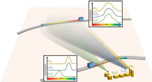
quan-Figure 1.Schematic of dual-tracer release technique. At distances far downwind (top), both tracers and CH4are spatiotemporally overlapped. At distances closer to the facility, the spatial position of the CH4plume relative to the two tracer plumes can indicate the location of an emission vector on-site with sub-facility resolution.
tities. The ratio of the two downwind concentrations is then equal to the ratio of flow rates:
1[CH4] 1[T] =
α α
FCH4 FT =
FCH4 FT
, (2)
whereFCH4 refers to the flow of CH4from the facility. Be-cause concentrations 1[CH4] and 1[T] are measured and FT is known,FCH4 can be determined without the need for detailed information aboutα.
The underlying assumption in this technique is that the tracer release point is located close enough to the unknown emission source that both gases experience the same dilution factorα. This separation distance becomes less important as the concentration measurement (aboard a mobile platform) moves further downwind. However, when the separation dis-tance is of the same order as the downwind disdis-tance, the α values associated with CH4andT are expected to be
signifi-cantly different. Under ideal circumstances, the tracer is col-located with the emission source, and their concentrations are measured far downwind in stable meteorological conditions. In practice this is not always possible due to facility size, in-terfering methane sources, road access, or varying winds.
To mitigate these issues, this study made use of a dual-tracer release technique (Allen et al., 2013) in which two different tracer gases, in this case N2O and C2H2, are
re-leased from different locations within the facility, bracketing the on-site equipment, as shown in Fig. 1. The use of a sec-ond tracer has two important advantages over single-tracer measurements. First, closer downwind measurements (50– 200 m downwind) afford a refined assessment of an emission source location based upon the position of its CH4plume
rel-ative to each tracer plume. Second, when conducting mixed plume characterization in the far-field (downwind), where αN2O∼αC2H2 ∼αCH4, the second tracer becomes an
inter-nal standard to the measurement. This capability mitigates the need for a calibration or for benchmarking against other measurements. Emissions rates determined by tracer release have, however, been compared to detailed on-site leak mea-surements in Subramanian et al. (2014). That study found that these two techniques usually agreed to within experi-mental uncertainty. The use of two known tracer gas flow rates and an observed downwind molar ratio also provides an empirical measure of the uncertainty for every plume. This error will be further described below, in the Supplement, and in the associated Measurements report (Mitchell et al., 2015).
2.4 Understanding and optimizing data quality
In the context of the two possible transect scenarios de-picted in Fig. 1 (spatially overlapping plumes vs. spatially separated plumes), it is important to qualitatively understand what measurement conditions (tracer separation, transect dis-tance, meteorology) yield these two results. This can be de-veloped using Gaussian dispersion modeling as a guide (Bey-chok, 2005). As a rule of thumb, for typical mid-day atmo-spheric conditions (stability classes A, B, or C, as described in the Supplement) and downwind distances (100–3000 m), the horizontal width of a plume that is propagating according to Gaussian dispersion is∼20–50 % of the distance that it has traveled from its source. That is, the ratio of plume width to downwind distance is 0.2–0.5, where low wind conditions yield wider plumes (∼0.5) and high wind conditions yield narrower plumes (∼0.2). A plume observed 1000 m down-wind of its origin, for example, is typically 200–500 m wide. If the plume widths of two gases being measured down-wind (e.g., CH4 and N2O) are much larger than the
distance between emission sources to the downwind tran-sect distance must be less than 0.2–0.5 in order to achieve co-dispersion. When, for example, the separation between an N2O tracer and a CH4 source is 100 m, the downwind
distance required to observe the onset of co-dispersion is > 500 m in high winds and > 200 m in low winds. Alterna-tively, when local road access limits the downwind distance to 200–500 m, the N2O tracer must be placed within 100 m
of the suspected CH4emission source.
This same rule-of-thumb approach can be applied to cases where a nearby CH4source, such as a wellhead, may
inter-fere with the FLER measurement at a G&P facility. In these cases, the downwind transect must be close enough that the interfering plume width is smaller than its separation from the G&P facility. For example, if the distance between a well-head and facility is 50 m, downwind transects must be less than 100–250 m in order isolate and exclude the wellhead plume from the FLER estimate.
When the second tracer is used as an internal standard, it can serve to quantify the uncertainty of the measurement. As will be shown below and in the Supplement, this uncertainty decreases when the two tracer plumes are spatially overlap-ping compared to cases where the plumes are separated. Be-cause this precision reflects the uncertainty in the FLER, efforts are made by the study team to maximize the co-dispersion of methane and tracer plumes. In light of the above discussion, this can be achieved by attempting to place one or both tracers near the dominant suspected emission source at a facility, when one exists. When these conditions are met, the downwind distance required to observe co-dispersion is reduced, thereby increasing the instrumental signal-to-noise and further separating any possible interfering sources.
Initial placement of the tracers at opposite ends of the fa-cility allows for early transects to identify suspected methane emission locations. In some cases, the observed methane plume will appear covariant with one of the two tracers, in-dicating that the dominant methane emitter is in the vicinity of that tracer. In many cases, however, the methane plume is observed between the two tracer plumes. In this scenario, one (or both) of the tracers is typically moved such that its plume is spatially overlapping the methane plume. This process is iterated multiple times over the course of the measurement in order to yield plumes that exhibit high degrees of CH4
-to-tracer correlation.
While two tracers act as an internal standard in the hor-izontal plane, a complicating factor unique to some large facilities (e.g., processing plants and larger gathering facil-ities) studied here is the presence of flares and/or engine ex-haust stacks, some of which can be over 20 m tall. Presented in the Supplement is a Gaussian plume and Brigg’s equa-tion analysis of the effect of a possible elevated CH4source
on the measured emission rate (Beychok, 2005). A simple rule-of-thumb approach as used above is hampered here by both buoyant plume rise effects and plume reflection off of the ground. These calculations indicate that in strong wind
conditions (i.e., high atmospheric stability classes, such as in winds above 5 m s−1), the measured emission rate
deter-mined from close transects can be biased considerably low, depending upon the fraction of the emission coming from el-evated positions. In wind conditions below 5 m s−1, the dis-persion is large enough that the bias is lessened to 0–50 %. To minimize this bias, plumes were obtained as far downwind as possible, and at several processing plants a tracer was emitted at an elevated position such as the side of a demethanizer col-umn or stack. The impact of the bias upon the overall data set and resulting conclusions is discussed in more detail in the accompanying Measurements paper (Mitchell et al., 2015). 2.5 Auxiliary species
The study team also used measurements of other species, CO, CO2, and C2H6, to aid in identifying and attributing
methane emissions to targeted G&P facilities. For exam-ple, engine exhaust from reciprocating engines and turbines that power compressors at many natural gas facilities will contain CO and CO2. This enables potential differentiation
between emissions of G&P equipment and those emanat-ing from nearby well pads (which typically do not include combustion sources or emit much smaller amounts of CO and CO2). Similarly, amine treatment systems serve as
non-combustion sources of CO2 and are easily distinguishable
from other facilities (Rochelle, 2009; EIA, 2006; Kidnay et al., 2011).
Ethane measurements serve multiple purposes within the context of this study. First, the presence of ethane associated with methane in downwind plumes indicates that some frac-tion of the methane is of thermogenic, rather than biogenic, origin. The ability to distinguish between these sources is es-pecially important in farming and ranching regions, where livestock emissions can be a substantial source of CH4.
Sec-ond, the observed ethane-to-methane ratio (E/M ratio) in a downwind plume can serve as a unique identifier of a facility of interest. It can therefore be used to differentiate a partic-ular emission source from others in the area. Finally, varia-tions in ethane content over close transects can indicate ac-tive distillation or other processing present on-site. The util-ity of these measurements will be explicitly illustrated via examples in the Results section.
3 Laboratory and instrument details
Table 1. Instruments and sensitivities for measured species on Aerodyne and CMU mobile laboratories.
Instrument Species detected Sensitivity
Aerodyne mobile laboratory
Aerodyne dual QCL CH4 1 ppb
C2H2 200 ppt
Aerodyne mini QCL C2H6 100 ppt
Aerodyne mini QCL N2O 100 ppt
CO 100 ppt
Li-Cor NDIR CO2 500 ppb
Carnegie Mellon mobile laboratory
Picarro CRDS CH4 3 ppb
C2H2 600 ppt
Aerodyne dual QCL C2H6 100 ppt
N2O 100 ppt
CO 100 ppt
et al., 2005) operating at 20–40 Torr are employed in series to detect CH4, C2H6, CO, N2O, and C2H2. To detect CO2, a
non-dispersive infrared (NDIR) LiCOR®instrument is used. In this work, the QCL spectrometers are operated in series, with flow rates through the instruments of∼10 SLPM. This flow rate afforded a time response of < 1 s. The NDIR in-strument draws a small flow from the inlet line before the air sample entered the QCLs. The QCL spectrometers re-port mixing ratios of all species in parts per billion by vol-ume (ppbv), while the NDIR instrvol-ument reports CO2in parts
per million by volume (ppmv). In the Carnegie Mellon mo-bile laboratory, CH4and C2H2are measured using a Picarro
cavity ring-down spectrometer (Crosson, 2008; Rella et al., 2009) running at 4–5 Hz, while C2H6, N2O, and CO are
measured using an ARI Dual QCL spectrometer operating at 1 Hz. Detection limits of all instruments are listed in Ta-ble 1. Except for practically limiting the minimum detectaTa-ble concentration of certain species, the differences in equipment manufacturer and sensitivity do not affect the results of the measurements. In addition to the concentration information, both mobile laboratories record their location, bearing, and heading using Global Positioning System (GPS; Garmin® 76 and Hemisphere GPS Compass®for the ARI laboratory, Airmar®for the CMU laboratory). A small meteorological station (Airmar® 200WX or LB150) is also mounted on a
boom at the front of the vehicle to record true wind speed (speed corrected for vehicle velocity), true wind direction (wind direction relative to true north), and GPS location. Along with the mixing ratios, this information is recorded at 1 s intervals on a main onboard acquisition computer, where all of the acquired data are visualized in real time and can be overlaid on maps.
Both laboratories are accompanied by a tracer release ve-hicle (i.e., pickup truck) to facilitate the storage, setup, and release of the N2O and C2H2tracers. Tracer gas bottles are
stored on the bed of the truck, along with flow control sys-tems and associated valves, tubing, and telemetry syssys-tems. Polyethylene tubing for each tracer is rolled out from the pickup truck up to 200 m to the intended release location, where the end of the tube is attached to on-site equipment or placed on a tripod. For both laboratories, tracer flow rates are controlled by Alicat® MC-series mass flow controllers. The mass flow rates are recorded via RS232 to an onboard computer in the vehicle.
In addition to the tracer gas flow systems, three portable meteorological stations (Airmar®200WX) are deployed on tripods, sometimes serving as physical supports for the tracer release tubing. They are capable of recording GPS, true wind direction, and wind speed with 1 s resolution. Each unit broadcasts that information wirelessly or via an RS232 ca-ble at 1 Hz to a computer onboard the tracer release vehi-cle, where it is recorded and displayed for observation by the tracer release personnel to advise the mobile laboratory as needed. When considered in the context of tracer placement, the wind data can immediately inform mobile laboratory per-sonnel whether a tracer is being deployed in an area on-site that is not well ventilated. If this is the case (frequently due to the local wind currents near buildings) the tracer can then be moved to allow it to be carried downwind by the larger regional wind mass. This information also provides a crude wind field for later analysis to better understand the sources of error and uncertainty in tracer release methods.
Calibrations and ranges
In both laboratories, the inlet was periodically overblown (in-jected with a flow larger than the intake flow) with ultra-zero air (AirGas®or Praxair®) to zero the instruments, typically every 15 min for 30 s. Because CH4and N2O are present in
background ambient air (1900 and 325 ppbv, respectively), zeroing events also serve as an approximate check of those instrument calibrations. Full instrument calibrations were performed several (4–5) times over the course of the mea-surement campaign using calibration standards. For these dilution calibrations, a controlled mass flow of calibration gas is released into a known zero-air flow, and the resulting mixture is overblown into the inlet. The mixture is changed by varying the calibration gas flow using either a series of critical orifices or mass flow controllers (Alicat® MC Se-ries). Typical calibration ranges were 0–10 ppm for CH4,
0–500 ppb for C2H2, and 0–1000 ppb for N2O. The
4 Field implementation
In practice, when the mobile laboratory arrived at a facility a safety meeting was conducted with the facility supervisor, after which the tracer release apparatuses were set up. The tracer positions were decided upon after discussion with the supervisor regarding likely emission sources (near compres-sors, dehydrators, tanks, etc.), a cursory survey with infrared imaging, consideration of the current wind conditions, site size and safety issues, and sometimes after performing an initial drive within facility boundaries. After setup, the tracer gases were released and the mobile laboratory was deployed downwind. Constant communication was maintained either over CB radio or cellular phones. During this period, an additional study team member (“the on-site observer”) sur-veyed the facility with an infrared camera, inventoried facil-ity components, and recorded relevant information such as facility throughput, equipment counts, and motor, engine, or turbine horsepower. In many cases the identification of emis-sion sources by survey of the facility using infrared imaging agreed with or informed the results of close-pass plume tran-sects. If the mobile laboratory detected CH4plumes that were
spatially separated from the tracer plumes, one or both trac-ers were moved to maximize co-disptrac-ersion with CH4. When
possible, on-site ethane-to-methane ratios were measured by driving the mobile laboratory within fence line immediately downwind (< 25 m) of on-site equipment, for future compar-ison with partner company gas chromatograph (GC) data.
After acquiring enough downwind plumes (a target of 10) to provide a statistically meaningful time-averaged FLER and uncertainty, the mobile laboratory returned on-site, and the tracer release hardware was packed. Usually at least two facilities were surveyed daily and sometimes as many as four, depending upon wind conditions, time, and the locations of nearby facilities. Because of their size and scale, a full day was reserved to sample emissions from processing facilities. 5 Plume types and analysis methods
There are multiple ways in which downwind tracer plumes can be analyzed, depending upon the plume intensity and spatial overlap between the tracer and CH4 plumes
(Sub-ramanian et al., 2014). Figures 2–5 show the four possible plume types observed during the G&P campaign.
5.1 Dual correlation
The ideal scenario occurs when the measurement transect is far enough downwind of the facility that the CH4, N2O, and
C2H2plumes are spatially overlapping. The resulting
mea-surements of concentration vs. time exhibit a high degree of covariance between species, as shown in the top panel of Fig. 2. Analysis of these “dual-correlation” plumes con-sists of plotting the concentration of one species vs. another and performing a linear orthogonal distance regression fit as shown in the bottom panels of Fig. 2. This regression analysis
is performed for CH4vs. N2O, CH4vs. C2H2, N2O vs. C2H2,
and C2H6vs. CH4. From these linear regressions, the slope
indicates the ratio of concentrations of the two gas species (for use in Eq. 2), andR2indicates the degree of correlation. These values are recorded for use in determining whether the plume meets the acceptance criteria for the CH4 emission
rate to be considered valid. If the R2 values derived from fits of CH4vs. N2O, CH4vs. C2H2, and N2O vs. C2H2are
all greater than 0.75, and the tracer ratio ([C2H2]/[N2O])
is within a factor of 1.5 of the known tracer flow rate, the plume is a candidate for dual-correlation analysis. The choice of acceptableR2and tracer ratio were based upon values at which further relaxation of the criteria would alter the uncer-tainty and accuracy of the FLER measurement (Mitchell et al., 2015). A discussion of the use of a factor for the tracer ratio criterion, as opposed to a deviation such as±50 %, is presented in the Supplement.
5.2 Dual area
In certain circumstances, wind conditions along with local road access and intervening CH4 sources prevent the
abil-ity to get far enough downwind for the tracer gas and CH4
plumes to become spatially overlapped. However, transects may still be performed closer to the facility (∼50–500 m) such that all three species will be observed. As illustrated in the example shown in Fig. 3, under these circumstances cor-relation diagrams do not provide useful information about the ratio of species (bottom panels). In these cases a “dual-area” technique is used, in which the analysis must rely on the integrated area of each species’ plume over the time of the transect. Here, the deviation of the species’ mixing ra-tios from ambient conditions must be considered, rather than the raw integrated intensity. This point is particularly rele-vant for CH4 and N2O, whose ambient concentrations are
∼1900 and ∼325 ppb, respectively. In the analysis of the data, the baseline (non-plume) mixing ratio was determined by fitting a line through the average of several data points im-mediately before the plume transect began and the average immediately after the transect ended. The fit line was then subtracted from the data to yield a baseline-corrected plume. This accounted not only for background concentrations (e.g., 1900 or 325 ppb) but also any minor baseline drift that may have occurred over the course of the transect. The quality of the baseline fit was visually confirmed and corrected if it did not accurately represent the true baseline. For the plume to be considered a candidate for dual-area analysis, the ratio of areas of the C2H2and N2O plumes must be within a factor
of 2 of the known tracer flow rates. 5.3 Single correlation
In scenarios where the CH4 mixing ratio was highly
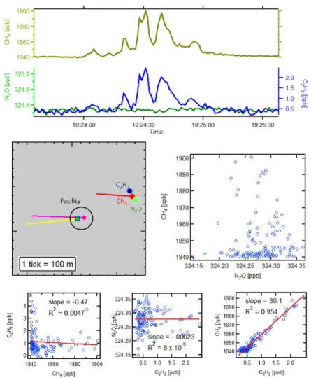
Figure 2.Example dual-correlation plume from a natural gas facility. Top panel: time trace of CH4, C2H6, N2O, and C2H2concentrations, showing high temporal correlation. Center left panel: map of tracer location (right side) and transect location (left side) during the course of the plume. Red, blue, and green weighted lines correspond to CH4, C2H2, and N2O intensities during the transect, spatially offset for clarity. Thin lines point into the wind at the mobile laboratory (red) and at the facility (light blue, pink, and yellow). Blue square and green triangle indicate C2H2and N2O release locations, respectively. Lower panels: Correlation analysis of C2H6vs. CH4, N2O vs. C2H2, CH4vs. C2H2, and CH4vs. N2O. The measured emission rate from this plume was found to be 3.4 SCFM.
corresponds to that originally used by Lamb et al. in early demonstrations of the tracer release method (Lamb et al., 1995). The need to use the single-correlation technique can be the consequence of several possible measurement condi-tions: (i) one of the tracers is placed geographically close to the dominant emitter within the facility (e.g., a compressor or large fugitive source), (ii) the site is emitting a tracer species (i.e., C2H2during certain combustion processes), forcing the
measurement to become single-tracer only, or (iii) the plume transect is far enough downwind (frequently > 2 km) that one of the tracer species’ mixing ratio is at or below the in-strumental detection limit. In single-correlation cases, cor-relation analysis is performed for both tracers but only the well-correlated tracer serves to provide the true CH4
emis-sion rate. For a plume to be a candidate for single-correlation analysis, theR2value derived from the linear regression fit of CH4to one of the two tracers must be greater than 0.75.
5.4 Linear combination of tracer plumes
In certain circumstances, unique tracer placement, road ac-cess, and wind conditions allow for intermediate-distance transects where the CH4plume profile is not well correlated
with either individual tracer but is well correlated with a lin-ear combination of the tracer plumes, i.e.,
1[CH4]=a·1[N2O]+b·1[C2H2], (3)
where a and b are multiplicative coefficients of the N2O and
C2H2 plumes, respectively. Such an example is shown in
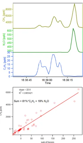
Fig. 5. This scenario is equivalent to performing two inde-pendent single-tracer measurements, where the plumes are overlapping in time. In these cases facility emission rates can be determined by performing a correlation analysis of CH4vs. (a·1[N2O]+b·1[C2H2]) while adjusting the
Figure 3.Similar to Fig. 2, illustrating dual-area-type plumes. Top panel: time trace of CH4, C2H6, N2O, and C2H2concentrations, showing high temporal correlation. Center left panel: map of tracer location (right side) and transect location (left side) during the course of the plume. Red, blue, and green weighted lines correspond to CH4, C2H2, and N2O intensities during the transect, spatially offset for clarity. Thin lines point into the wind at the mobile laboratory (red) and at the facility (light blue, pink, and yellow). Blue square and green triangle indicate C2H2and N2O release locations, respectively. Lower panels: correlation analysis of C2H6vs. CH4, N2O vs. C2H2, CH4vs. C2H2, and CH4 vs. N2O. Note the lack of correlation in lower left and center panels, indicating that the analysis must rely on an area method. Note, however, the strong correlation between C2H6and CH4(bottom left), indicating that the observed methane is derived from natural gas. The emission rate determined from this plume was found to be 3.1 SCFM.
the CH4emission rate associated with each tracer. While the
sum of these values serves as the FLER, the individual emis-sion rates contain information at sub-facility-level resolution, such as leak or vent magnitudes associated with condensate tanks, compressors, or dehydrators.
This analysis method has also been applied in cases where equipment not associated with the G&P (e.g., a natural gas production well) is present within a facility boundary. In such a case, one tracer is placed at or near the non-associated equipment while the other is placed near a suspected emit-ter that is part of G&P facility. If the plume from the former tracer is well correlated with the non-associated equipment emission and the plume from the latter tracer is well corre-lated with the rest of the CH4 from the facility of interest,
then the facility level emission rate can be estimated, even
when the CH4 from the non-associated equipment is
over-lapping with the facility plume.
5.5 Implementation of plume analysis
Table 2 summarizes the preference of the four analysis meth-ods, their acceptance criteria, the number of accepted plumes that were analyzed using each method, and the measurement variance associated with each plume type. The determination of the variance for each plume type is discussed in detail in the Supplement.
Figure 4. Example of a single-correlation plume (CH4correlation with C2H2). Top panel: time trace of CH4, C2H6, N2O, and C2H2 concentrations, showing high temporal correlation. Center left panel: map of tracer location (right side) and transect location (left side) during the course of the plume. Red, blue, and green weighted lines correspond to CH4, C2H2, and N2O intensities during the transect, spatially offset for clarity. Thin lines point into the wind at the mobile laboratory (red) and at the facility (light blue, pink, and yellow). Blue square and green triangle indicate C2H2and N2O release locations, respectively. Lower panels: correlation analysis of C2H6vs. CH4, N2O vs. C2H2, CH4vs. C2H2, and CH4vs. N2O. The emission rate determined for this plume was found to be 8.1 SCFM.
yields variances for each plume type, the inverses of which are used as weighting factors for determining the weighted-average FLER. Not surprisingly, the dual-correlation method exhibits the lowest variance of all plume types and is there-fore the most preferred. This is likely due to the fact that these plumes correspond to a limit where full co-dispersion of the tracers has been achieved, i.e., both tracer plumes are experiencing the same local turbulence by the time they are measured by the mobile laboratory. In addition, no baseline subtraction is required in the dual-correlation method, which can be a source of uncertainty depending upon the signal-to-noise exhibited by the plume. The larger variance of the dual-area method is likely derived from the lack of co-dispersion of the tracers. In these scenarios, one tracer concentration may be enhanced relative to the other due to the fact that each tracer plume is experiencing different local turbulence en route to the mobile laboratory.
Table 2.Plume analysis types, preference, criteria, prevalence, and variance.
Analysis type Preference Criteria # of Variance plumes (√variance)
Dual correlation 1 – R2>0.75: N 250 0.04 (0.2) 2O vs. C2H2, N2O vs. CH4,
C2H2vs. CH4, C2H6vs. CH4
– Tracer ratio error<1.5
– E/M ratio error<1.5
Dual area 2/3 – R2>0.75: C 441 0.14 (0.37) 2H6vs. CH4
– Tracer ratio error<2
– E/M ratio error<1.5
Single correlation 3/2 728 0.09/0.22
(0.3/0.47)
– R2>0.75: C2H6vs. CH4, Tracer vs. CH4
– E/M ratio error<1.5
Linear combination 4 – R2>0.75: C 16 – 2H6vs. CH4
5.6 Ethane-to-methane ratio
Finally, the ratio of ethane to methane in the measured down-wind plume can also serve as an acceptance criterion regard-less of plume classification. The amount of ethane in a nat-ural gas mixture can vary from well to well and from one gathering facility to another (Kidnay et al., 2011). As such, the ethane content represents a unique “fingerprint” of a fa-cility, providing a means to identify whether the CH4
mea-sured in a plume is coming from the facility of interest. In this study, the ethane-to-methane ratio (E/M ratio) associ-ated with a given facility was determined in one of two ways: from partner company GC analysis of the inlet/outlet gas or from C2H6vs. CH4correlation analysis of plumes when the
mobile laboratory was on-site (and thus only observing emis-sions from the facility). While GC analysis data are preferred since they provide a completely independent (and external) check of the methodology, they were not always available on the date of the measurement. When possible, observed E/M ratios of plumes obtained when the mobile laboratory was on-site were compared to the GC data to confirm (or dis-prove) that the emission composition was in agreement with the GC data.
Both mobile laboratories measured ethane and methane at a 1 Hz sampling rate or faster, allowing for an accurate deter-mination of the E/M ratio of individual plumes. The E/M ratio for every downwind plume obtained in the campaign (determined using correlation analysis) was measured and compared to the known ratio from GC analysis (or measured on-site E/M ratio in cases where the GC data were unre-liable). A detailed comparison between the observed E/M ratio and that from the inlet GC analysis is presented in the
results section. A plume was only accepted for further anal-ysis when the observed ratio was within a factor of 1.5 of the known value. This criterion was suspended in cases where the facility itself was actively changing the ethane content (e.g., from a demethanizer), where the E/M ratio was vary-ing across the facility, or when the downwind C2H6mixing
ratio was below the detection sensitivity limit.
Finally, under certain scenarios, a small number of plumes that would be rejected as described above are manually ac-cepted during analysis. These exceptions are possible for one of several reasons. One is that the plume transect is far enough downwind that the tracer or CH4 plume
concentra-tions are near the detection limit of the onboard instruments. Under such a scenario the correlation analysis may reveal R2< 0.75 despite the plume being legitimate. Another possi-ble reason for manually accepting a plume is when the E/M ratio is variable across the facility, which is frequently due to the presence of a high emission point source such as a venting condensate tank. Because condensate tank emissions may exhibit an E/M ratio larger than that of the remainder of the facility, the observed downwind ratio may be variable, even on the timescale of a single plume.
6 Results
In this section, we present results from a number of case stud-ies that illustrate the capabilitstud-ies of the dual-tracer release method.
6.1 Gathering facilities
high-Figure 5.Example of analysis using a linear combination of tracer plumes. Note that N2O and C2H2are associated with different sec-tions of the CH4 plume (top). Adding the two tracer plumes in an 81/19 % combination yields a correlation diagram (below) with highR2value (0.87). The emission rate determined from this plume is 56.1 SCFM.
pressure stream of gas. These facilities typically include equipment such as inlet separators to remove liquid phase water and condensate (C5+), when present, and systems for
pipeline maintenance activities (e.g., “pigging”). Compres-sion at these facilities is accomplished by a series of 1 to 20 individual compressors powered by electric motors, recipro-cating engines, or gas turbines with total engine powers rang-ing from 500 to 25 000 HP dependrang-ing on the inlet gas pres-sure and total gas throughput (Mitchell et al., 2015). Gather-ing stations also typically contain condensate storage tanks, produced water storage tanks, and other gas handling equip-ment including pneumatic valves (often powered by natural gas) and gas metering systems. If the gas has a high wa-ter content, glycol dehydration systems are also frequently present to dry the gas (Goetz et al., 2014; Kidnay et al., 2011).
There are three main sources of continuous emissions from these facilities. First, compressors can serve as significant sources of CH4 via both fugitive leaks as well as through
seals in the compressor housing. In the case of wet com-pressor seals, it should be noted that the primary emission
route is due to absorption of methane into the seal fluid at high pressure, followed by exposure of the fluid to ambient pressure, where the methane is routed through a vent to at-mosphere (EPA, 2006). Second, because the natural gas is typically under high pressure, fugitive and vented emissions may occur at the facility, including from continuous-bleed natural gas pneumatic devices, dehydration units, and a vari-ety of flanges and valves. Third, methane slip (i.e., unburned methane in engine exhaust gases) through on-site combustion sources such as engines and turbines can be a source of CH4,
depending upon a wide variety of combustion characteristics. The relative importance of this emission source to the FLER is discussed in the associated Measurements report (Mitchell et al., 2015) and in previous studies of combustion emissions in natural gas transmission and storage (Subramanian et al., 2014). Similarly, methane and other unburned hydrocarbons are present in flare emissions and may vary greatly depend-ing upon the flare combustion efficiency (Torres et al., 2012). Some intermittent methane emission sources may also be found at gathering facilities, such as intermittent-bleed nat-ural gas-driven pneumatic controllers, produced water tanks, and condensate tanks. Of particular importance to the asso-ciated Measurements paper (Mitchell et al., 2015), produced water and condensate tanks may transiently emit CH4, C2H6,
and higher hydrocarbons from thief hatches or other pres-sure relief valves attached to the tank. Because of the nature of the liquids stored in them, i.e., long-chain hydrocarbons, the ethane-to-methane ratio observed from a condensate tank can be much higher than the natural gas composition entering or exiting the facility. However, these units may sometimes also serve as venting release points for equipment on-site, in which case the E/M ratio will be very similar to that of the inlet stream.
An example of an emission rate measurement from a com-pressor station (C station) is shown in Fig. 6a. Similar to the example plume shown in Fig. 2, this plume as accepted as dual correlation (R2=0.998, tracer ratio error=1.05, E/M ratio error=1.4). The average emission rate from this facility was found to be 43.8±8.4 kg h−1. In this case, the methane and ethane signals are strongly correlated with both tracers at a distance of 1600 m downwind of the facility. Note that inclusion of the CO and CO2in the analysis indicates that
both of these gases are also being emitted from the facility, likely due to combustion. While this plume alone can pro-vide an accurate determination of the FLER from the facil-ity, even more information can be extracted by also investi-gating transects from only 100 m away, shown in Fig. 6b (a dual-area plume, with tracer ratio error=0.7, E/M ratio er-ror=1.5). While such a close transect may not provide as precise a FLER, we see from the figure that the CO and CO2
signatures are coincident with only a fraction of the methane being emitted and are not well correlated with it. This indi-cates that some, but not all, CH4emitted at the facility may
Figure 6.Three exemplary plumes from a gathering station:(a)far-field plume (1.6 km) showing strong correlation between CH4, C2H6, N2O, C2H2, CO2, and CO;(b)close plume transect (100 m away) of same facility, showing loss of correlation and isolation of CO2and CO combustion products to a section of the facility;(c)example of a close plume transect (200 m away) showing CO and CO2correlation with a component of the CH4trace.
Figure 7.Example of varying E/M ratio during a close transect
due to the presence of a condensate tank battery on-site. Note the
∼2×decrease in the E/M ratio toward the end of the plume.
on-site. At some facilities, such as that shown in Fig. 6c, CO and CO2are correlated with a distinct part of the CH4plume,
indicating the presence of a combustion source that is emit-ting CH4or co-located with one that is and clearly associated
with one section of the facility. Because the goals of the G&P study are to understand both overall emissions and their ori-gins, this type of analysis can aid in understanding the rel-ative role of combustion sources and methane slip in G&P CH4emissions. In the case of the compressor station
associ-ated with the plume in Fig. 6c, the area of the facility with CO, CO2, and CH4emissions is the compressor/engine
sec-tion, while the area with no CO/CO2corresponds to other
non-combustion sources on-site. Thus, Fig. 6 illustrates the important role that the auxiliary gas measurements (in this case CO and/or CO2)can play in identifying sources of
emis-sions.
Because they are ubiquitous at both production and gather-ing facilities, it is of interest to this study to understand, and quantify when possible, what fraction of emitted methane is coming from condensate and produced water tanks. Shown in Fig. 7 is an example of the emission profile observed at a compressor facility containing a condensate tank, illustrating another example of the utility of close (< 200 m) transects. In this case, one tracer (N2O) was placed next to the
com-pressors, while another (C2H2)was placed near a battery of
three condensate tanks. As shown in the transect trace, both of these sources (compressors and tanks) are correlated with their respective tracers but have very different E/M ratios. Here the relative intensities of the CH4 plumes associated
measurement of auxiliary species such as ethane, provides the ability to address the contributions of particular equip-ment, especially condensate tanks, to emissions from G&P facilities. Here, for example, analysis using a linear combina-tion of tracers as described above reveals that the CH4
emis-sion from the condensate tank represents 50 % of the overall CH4emission rate from the facility. The average total
emis-sion rate from this facility was found to be 48±22 kg h−1. While not always the case, it is common to find a larger ethane content in emissions from condensate tanks relative to the inlet gas composition due to the larger fraction of ethane in the condensate itself. It should be noted that daily tem-perature variations (producing “breathing” emissions) may change the relative vapor pressures of ethane and methane in the condensate tank, and the filling/emptying schedule of the condensate tank (producing “working” emissions) may alter condensate composition. Both of these activities can there-fore change the E/M ratio of the tank emissions over the course of the day.
6.2 Amine treatment
The composition of natural gas often depends upon its ge-ologic origin (or play). To illustrate this effect, we com-pare emissions from facilities associated with different gas sources: shale and coal bed methane (Whiticar, 1994; Kidnay et al., 2011). Shale gas, tight gas, and conventional gas con-tain varying amounts of ethane and higher hydrocarbons, typ-ically with low levels of CO2. Coal bed methane, however,
typically contains little ethane and up to 40 % CO2(Kidnay
et al., 2011). This carbon dioxide is particularly interesting since in this case it is not an indicator of combustion. Other combustion sources within the facility can be distinguished by the presence of CO.
If CO2is present in high amounts (> 3 %), it must be
re-moved from the natural gas prior to transmission and storage. It can be removed from a gas stream by passing the natu-ral gas through a vapor of monoethanolamine or other re-lated amine compounds. This process is called “amine treat-ment” or “amine scrubbing” (Kidnay et al., 2011; Rochelle, 2009; Bottoms, 1930). The amine binds to the CO2 and is
then regenerated through heating. CO2is thus evolved from
this process, so the facility’s CO2emissions relative to CH4
will be higher than would be expected for a direct leak of the untreated gas. Heating is applied through combustion of excess fuel (natural gas or other easily available source) so CO2may sometimes be present along with small amounts of
combustion products such as CO and NOx. Amine treatment is also used for the removal of hydrogen sulfide (H2S), with
the main difference being that the H2S is highly toxic and
must be captured or combusted.
Figure 8 contrasts emissions from facilities associated with coal bed methane and shale gas. The facility in Fig. 8a is a coal bed methane treatment plant without compression. The average emission rate from this facility was 142±50 kg h−1.
The compressor/dehydration facility shown in Fig. 8b (the same compressor facility discussed above) had four com-pressors and is in a shale region with characteristically high ethane content in the gas. The ethane content of the coal bed methane is observed at a molar ratio C2H6/CH4=0.0215
(Fig. 8a), while the shale-gas facility emissions have a much higher measured ratio, C2H6/CH4=0.164 (Fig. 8b). The
CO2 emissions vary even more greatly between the
facil-ities, at CO2/CH4=165 vs. CO2/CH4=3.3. The
mo-lar ratio of CO2 to CH4 in the former facility’s emissions
(CO2/CH4=165) is 4 orders of magnitude higher than the
operator data for the inlet gas (CO2/CH4 =0.106). For
Fig. 8a, at the distances sampled no other significant com-bustion products (such as CO) were observed, indicating that the primary source of CO2is the amine treatment process.
This information, along with the observed high degree of correlation between CO2and CH4at intermediate distances
(∼500 m), suggests that the primary CH4emission source is
located within or near the amine treatment area of the facility. 6.3 Natural gas processing
Natural gas processing plants are large, complex facilities that remove unwanted compounds in the incoming gas stock (e.g., H2S, CO2, H2O) and separate other high-value
com-pounds (i.e., natural gas liquids, as discussed below) from the gas to produce pipeline-quality natural gas. Physically, processing plants often serve as the nexus between the gath-ering networks in the area and a transmission system work-ing to serve longer-range transport. They are typically char-acterized by capacity throughputs of 3–1500 million stan-dard cubic feet per day (MMscfd; equivalent to 2400– 1 200 000 kg h−1). The types of equipment and the processes
that are undertaken at a gas-processing plant depend on the composition of the gas in the region. Many plants utilize multiple processing “trains” to enable flexible operation. The equipment and steps in each train can vary depending again on the region and the engineering decisions made by the operator of the plant (Kidnay et al., 2011). It should also be noted that not all natural gas in the US supply chain is processed. Rather, in cases where natural gas composition does not contain substantial levels of natural gas liquids or H2S/CO2(i.e., is dry and sweet), the natural gas flows
di-rectly from gathering facilities into transmission pipelines (and sometimes directly into distribution networks).
The initial process that is typically found at a gas-processing plant involves a continuation of the treatment types found in the gathering system of the region. At some facilities, the initial product will be a first cut at collecting natural gas condensate, which is typically comprised of func-tionalized hydrocarbons above C5, using an inlet separator
Figure 8.Example of differing CO2plume profiles as a function of gas play:(a)emissions from a plant in a coal-gas region, with an amine scrubbing unit, showing significant CO2emissions; and(b)emissions from a gathering facility with no treatment in a shale-gas region.
effective continuous regeneration. As discussed below, natu-ral gas liquids are removed from the gas stream using either a cryogenic separation or separation based on solubility in lean oil (Kidnay et al., 2011). Additional details of this class of compounds and specific equipment used are discussed in the next section.
Due to the nature of the various processing steps and types of equipment found at processing plants, as well as the some-what larger geographic scale they typically occupy, there are typically multiple methane emission points with various co-emitted compounds. On the surface, this type of source is a direct challenge to the tracer release methodology given the constraint for the controlled tracer release to be as close to the emission source as possible. The following examples and discussion describe how these types of facility are quantified using the dual-tracer methodology as well as using the nature of the co-emitted compounds to deduce the dominant emis-sion sources.
The geographic scale of processing plants presents a chal-lenge to the dual-tracer flux ratio quantification given the constraints of wind direction and roadway access. Figure 9 depicts a pair of transects from a processing plant. The av-erage emission rate measured at this plant was found to be
128±66 kg h−1. Each transect was collected with the mo-bile lab maneuvering from north to south. This is depicted by the rainbow bar in each of the two split time series (a) and (b) in the left hand panel and portrayed on the right-hand panel with the relative distance (north vs. east). In the case where the transect was captured at the facility fence line (a), we see relatively high spikes in plume mixing ratios with three different quantifiable E/M ratios. Note that the tracer release locations were relatively close to one another and this is reflected in the spatial coherence in both of the transects.
In the case of the more distant (∼1.2 km) transect, the mixing ratios of ethane and methane are significantly less spiked. Careful analysis of the time and space dependence of the E/M ratio suggests that even at this distance the ratio in the northern sector of the facility is different than that in mid-dle and southern sections. This observation is corroborated anecdotally by the physical location of the liquids storage and natural gas transmission hardware on-site. In this facility the recompression of pipeline-grade natural gas takes place in the southern third of the facility. This corresponds to the lowest E/M ratio (red-purple in the time series) but is a sig-nificant source of CH4emissions (∼50 %) from the facility.
Figure 9.In the left-hand panel, the time series for methane, ethane, nitrous oxide, and acetylene are depicted for two transects,(a)and(b). In the right-hand panel, the geographic location is portrayed for the processing plant (grey) and the two transects(a)and(b). See text for additional discussion.
section of the facility. The effective leak rate of methane is less than in other sections of the facility because the methane is at residual levels in the liquids headspace. The E/M ratio in the green and yellow section of the time series is greater because this is where the NGL stock is being processed.
To quantify the FLER from processing facilities, fre-quently the dual-area analysis method is used. In the case of the close transects, the measured methane emission rates often exhibit substantial variance. The average of multiple close transects typically was found to be comparable to val-ues determined by more distant, better-mixed plume inter-cepts, when such a comparison was available.
6.4 Natural gas liquids and condensates
NGL is an umbrella term (EIA, 2013) for the many differ-ent chemicals and blends extracted in the liquid form from natural gas. Depending on the equipment available and the demand for the various products, the amount of processing of natural gas can vary greatly. At the lower end of the spec-trum, the gas may undergo dehydration and just enough re-moval of C2+ to meet pipeline specifications, such that no
liquids condense at pipeline pressures. Removal of other im-purities such as CO2and H2S may also be required to meet
pipeline specifications. At the highest end of the processing spectrum, cryogenic distillation will be employed to sequen-tially extract methane (demethanizer), ethane (deethanizer), propane, iso- and n-butane, and higher hydrocarbons. This processing can occur at a single facility or can be performed in several steps between different facilities. The net result is to separate the methane (and/or ethane) from other condens-able compounds that may still be present in the feed stock after the various upstream treatments. The liquid product at this stage is referred to as “x” or “y” grade liquid depend-ing on the cut temperature and ethane content in the uid. In some of the processing plants in this study, this liq-uid stream is stored in this state and shipped off-site via an NGL pipeline or tanker truck. In other facilities studied, the liquid is further fractionated, sequentially removing ethane,
then propane, then butane (Kidnay et al., 2011). Because of the low methane content within the liquid, this further pro-cessing of the NGL is not expected to significantly contribute to the FLER but may play a role in the E/M ratio that is ob-served downwind.
Many of the facilities visited in this study were in so-called “ethane rejection” mode, meaning that distillation towers were operated at lower liquids recovery levels and purified ethane is treated as a byproduct of the C3+ extraction. As a
byproduct, it frequently was re-injected into the natural gas stream. This occurs when there is less demand for purified ethane as a feedstock for ethylene, a process that occurs at an extremely limited number of locations in the US.
As in the case of identifying condensate tank emissions, the E/M ratio can inform the attribution of a methane emission source to individual pieces of NGL equipment. A striking example is shown in Fig. 10. This facility has two compressors, dehydrators, condensate tanks, and processing equipment. The measured CH4emission rate from this
facil-ity is 58±22 kg h−1. The nitrous oxide tracer (green marker) was placed near the condensate tanks and the acetylene tracer (blue marker) near the compressors. Northeast of the acety-lene tracer, above-ground piping marks the facility’s inlet and outlet (natural gas) as well as a liquids pipeline carrying a mixture of ethane and propane produced at the facility. The E/M ratio for the mixed facility plume was 0.0576, while the ratio for the liquids pipeline and inlet/outlet region was 14.58, i.e., nearly entirely ethane. Therefore, this transect in-dicates that the pipeline is not a significant source of CH4
emissions.
Fig-Table 3.Measured E/M ratios as a function of gas type at gathering and processing facilities. Minimum, median, and maximum average measured ratios are noted. Offshore gas is not included here due to the small number of offshore facilities measured.
Gas type Measured E/M ratio
min median max count
Coal bed methane 0.00 0.014 0.045 8
Coal bed methane 0.0057 0.018 0.031 4
and conventional
Shale 0.0055 0.051 0.24 64
Conventional 0.012 0.068 0.22 37
Figure 10. Downwind plume transect showing mixing ratio as a
function of time (top) and a map (bottom). Tracer release loca-tions are shown as a green triangle (nitrous oxide) and a blue square (acetylene). The plume transect is colored by methane mixing ratio (black to yellow). Ethane mixing ratio is also shown with a geo-graphic offset. Wind vectors (pink, red, and yellow) point into the wind.
ure 11 shows a comparison between the measured E/M ra-tios at each facility and the operator-provided data on gas composition. Agreement is good overall, with a few outliers. Also shown in the figure are 95 % confidence limits on the measured E/M ratios. Large error bars in the facility average for E/M ratios are usually due to variations in the emission composition, since the error for any individual ratio measure-ment is low. The operator gas composition information was not always measured on the same day as the field testing. For gathering facilities, gas composition is periodically mea-sured by gas sampling and subsequent third-party analysis.
Figure 11.Comparison between measured ethane/methane ratio
and operator data on gas composition. Error bars correspond to the 95 % confidence limits from the replicate experimental plumes. Points are also colored by the type of gas at each site. A line to guide the eye is drawn at a 1 : 1 correspondence between measured and operator data.
For processing plants, gas composition data are typically ac-quired in real time at multiple locations at the facility. In ei-ther case, the gas composition exiting the gaei-thering facility or processing plant may not always reflect the gas composition of the emission sources. This can be due to the E/M ratio changing as the gas moves through the facility or from emis-sions from condensate/produced water tanks. This variety of equipment and processes at gathering facilities and process-ing plants explains much of the discrepancy between mea-sured and operator E/M ratios compared to the transmission and storage study, where the composition of the gas does not vary during handling (Subramanian et al., 2014; Yacovitch et al., 2014). Table 3 outlines the minimum, median, and max-imum facility average E/M ratios divided by primary gas type. It should be noted that the classification by gas type is not rigid. That is, there may be multiple gas types other than the primary present at these facilities. The points in Fig. 11 are colored based on this gas classification. As noted above, coal bed methane facilities typically have the lowest E/M ratios. Conventional facilities sit somewhere in the middle, with the shale-gas facilities split into several clusters. The shale gas is scattered about the plot, with some clustering associated with various geographic basins. The three main shale clusters observed in Fig. 11 (green points) correspond loosely to: the Denver (Denver–Julesburg), Permian (Eagle Ford and Delaware), and Appalachian basins (∼12–23 %); the Anadarko (Mississippian Lime gas play), Uinta (Natu-ral Buttes), and Piceance basins (∼4–6 %); and the Arkoma basin (∼1 %). Other shale basins were also visited but the number of facilities for each of these basins is low.
7 Conclusions