www.atmos-chem-phys.net/15/595/2015/ doi:10.5194/acp-15-595-2015
© Author(s) 2015. CC Attribution 3.0 License.
Multiday production of condensing organic aerosol mass in urban
and forest outflow
J. Lee-Taylor1, A. Hodzic1, S. Madronich1, B. Aumont2, M. Camredon2, and R. Valorso2 1National Center for Atmospheric Research, Boulder, CO 80307, USA
2Laboratoire Interuniversitaire des Systèmes Atmospheriques, UMR 7583, CNRS, Université Paris Est Créteil et Université Paris Diderot, 94010 Créteil, France
Correspondence to:J. Lee-Taylor ([email protected])
Received: 11 May 2014 – Published in Atmos. Chem. Phys. Discuss.: 3 July 2014 Revised: 5 November 2014 – Accepted: 2 December 2014 – Published: 16 January 2015
Abstract.Secondary organic aerosol (SOA) production in air masses containing either anthropogenic or biogenic (terpene-dominated) emissions is investigated using the explicit gas-phase chemical mechanism generator GECKO-A. Simula-tions show several-fold increases in SOA mass continuing for multiple days in the urban outflow, even as the initial air parcel is diluted into the regional atmosphere. The SOA mass increase in the forest outflow is more modest (∼50 %) and of shorter duration (1–2 days). The multiday production in the urban outflow stems from continuing oxidation of gas-phase precursors which persist in equilibrium with the par-ticle phase, and can be attributed to multigenerational reac-tion products of both aromatics and alkanes, especially those with relatively low carbon numbers (C4–15). In particular we find large contributions from substituted maleic anhydrides and multi-substituted peroxide-bicyclic alkenes. The results show that the predicted production is a robust feature of our model even under changing atmospheric conditions and dif-ferent vapor pressure schemes, and contradict the notion that SOA undergoes little mass production beyond a short ini-tial formation period. The results imply that anthropogenic aerosol precursors could influence the chemical and radia-tive characteristics of the atmosphere over an extremely wide region, and that SOA measurements near precursor sources may routinely underestimate this influence.
1 Introduction
The contribution of anthropogenic aerosol is one of the great-est current uncertainties in the assessment of climate forcing (e.g., Forster et al., 2007). Organic aerosol (OA) comprises a significant (20–90 %) fraction of anthropogenic aerosol (Kanakidou et al., 2005; Jimenez et al., 2009; Zhang et al., 2007). OA consists, to a first approximation, of both pri-mary organic aerosol (POA) directly emitted as particles in evaporative equilibrium with the gas phase (Robinson et al., 2007) and the much more abundant secondary organic aerosol (SOA) produced by condensation of oxidation prod-ucts of gas-phase VOC (volatile organic compound) precur-sors (e.g., Kanakidou et al., 2005; Jimenez et al., 2009). Cli-mate uncertainties stem from both the difficulty in character-izing the radiatively important interactions of OA given its globally nonuniform composition (McFiggans et al., 2006), and from the difficulty in simulating its abundance and dis-tribution (e.g., Goldstein and Galbally, 2007; Hallquist et al., 2009).
aerosols acting as cloud condensation nuclei (CCN). The re-lationship between CCN number and radiative forcing is it-self complex and model parameterizations vary substantially (Boucher et al., 2013). Recent studies attribute about one-third of the total uncertainty in modeled CCN concentrations to uncertainties in SOA production (Carslaw et al., 2013), and find that CCN concentrations are sensitive to the relative proportions of POA and SOA (Trivitayanurak and Adams, 2014) and to oxidative ageing (Yu, 2011). These results show the importance of representing sources and life cycle pro-cesses that affect the mass and other climate-relevant prop-erties of SOA in as realistic and physically based a way as possible.
Laboratory-based descriptions of SOA formation and yields have become increasingly complex. Early calculations used precursor-specific two-product formulations (Odum et al., 1996), which describe smog chamber OA mass yields reasonably well but produce significant underestimates of atmospheric OA in both near-source regions and in the free troposphere (e.g., Volkamer et al., 2006; Heald et al., 2011). The VBS (volatility basis set) framework (Donahue et al., 2006) uses empirical volatility distributions to describe multi-species particle–gas mixtures and their chemical trans-formations (ageing) over laboratory timescales (Grieshop et al., 2009; Robinson et al., 2007). This concept broadly des-ignates SVOCs (semi-volatile organic compounds), species with significant fractions in both gas and particle phases, and IVOCs (intermediate-volatility organic compounds), gas-phase species whose products are likely to condense as SOA (Donahue et al., 2009). VBS formulations have improved SOA estimates in numerous model studies (e.g., Tsimpidi et al., 2010; Lane et al., 2008; Dzepina et al., 2011; Zhang et al., 2013). However the ageing parameterizations are of-ten tuned to match observed OA mass distributions (e.g., Jo et al., 2013), and as such are not generalizable. In efforts to incorporate more chemical complexity and realism to rep-resentations of bulk organic aerosol properties and evolu-tion, various two-dimensional schemes have been developed (e.g., Kroll et al., 2011; Donahue et al., 2012; Pankow and Barsanti, 2009; Barsanti et al., 2013) and implemented in re-gional (e.g., Murphy et al., 2012) and global (e.g., Mahmud and Barsanti, 2013) models. Other model studies have in-creased the number of OA precursor types represented (e.g., Pye and Pouliot, 2012), or added SOA production in cloud drops (e.g., Lin et al., 2012). These modeling advances have reduced, but not eliminated, the gaps between predictions and ambient measurements of SOA.
The difficulty in reproducing observed aerosol mass dis-tributions is partly attributable to the mismatch between the timescales accessible to laboratory studies, and the atmo-spheric lifetimes of OA and its precursor gases. OA life-times are generally considered to be of the order of about a week (Boucher et al., 2013) or more (Kristiansen et al., 2012), during which the airborne particles are continually subject to ageing processes. The dynamic nature of gas–
particle condensation equilibria (Pankow, 1994b) allows for evaporation–oxidation–recondensation cycling of OA con-stituents, altering the chemical composition including the rel-ative proportions of POA and SOA. In addition, the con-tinual chemical evolution of the associated gas phase im-plies product volatility changes on timescales of several days (Kroll and Seinfeld, 2008), opening the possibility of mul-tiday SOA formation. By contrast, practical considerations typically limit aerosol chamber studies to a few hours, al-though a few recent studies have achieved effective photo-chemical timescales of up to 3 days (e.g. Yee et al., 2012; Craven et al., 2012). Field observation of long-term aerosol evolution is also challenging owing to dilution and mixing of outflow plumes with regional air. SOA production in various plumes has been assessed by normalizing OA to1CO, the difference between plume and background CO values (e.g., Kleinman et al., 2008; DeCarlo et al., 2010; and references therein). Such observations generally extend to photochem-ical ages of∼1 day (DeCarlo et al., 2010). Ship-borne OA and CO observations in urban plumes with transport-based ages of up to about 4 days have clearly shown SOA produc-tion for∼2 days, with large data scatter thereafter (de Gouw et al., 2008).
Another problem of scale is inherent in the sheer number of potential chemical reactions and products leading to SOA formation (e.g., Goldstein and Galbally, 2007). Indeed, re-cent advances in high-resolution mass spectrometry analyt-ical techniques have enabled characterization of many hun-dreds of individual OA constituents (e.g., Nizkorodov et al., 2011, and references therein; Chan et al., 2013; O’Brien et al., 2013; Kourtchev et al., 2014). Explicit modeling of hy-drocarbon chemistry involves potentially millions of inter-mediate species (Aumont et al., 2005). This can be simpli-fied to only a few hundred species when considering ozone production (Szopa et al., 2005), but is far more complicated for SOA production (Camredon et al., 2007; Valorso et al., 2011; Aumont et al., 2012, 2013), which is not dominated by any one species but rather results from condensation of many oxygenated intermediates and their in-particle trans-formations.
of our model, and to elucidate the chemical identities of the species responsible.
2 Approach
2.1 The GECKO-A model
GECKO-A (Generator of Explicit Chemistry and Kinetics of Organics in the Atmosphere) is an automatic generator for atmospheric gas-phase chemical mechanisms. It is described in detail by Aumont et al. (2005), with updates by Camredon et al. (2007), Aumont et al. (2008), and Valorso et al. (2011), and as described here. The atmospheric oxidation of aliphatic compounds is treated explicitly based directly on laboratory measurements if available, or on structure–activity relation-ships (SARs) where data are not available. The chemical mechanism for the oxidation of aromatic compounds is taken from the Master Chemical Mechanism, MCM v3.1 (Jenkin et al., 2003; Bloss et al., 2005a), up to the loss of the aromatic structures, and computed from GECKO-A for subsequent chemistry. Photochemistry is driven by aj-value lookup ta-ble, calculated using the TUV (Tropospheric Ultraviolet Vis-ible) model (Madronich and Flocke, 1998).
In this study we implement GECKO-A in a similar man-ner to that described by L-T11, with the following modifi-cations. We have implemented the SAR of Vereecken and Peeters (2009) for alkoxy decomposition rates as described in (Aumont et al., 2013), we modified the SAR for hydro-gen abstraction from aldehydes, based on the study by Baker et al. (2004); we added oxy-radical production channels for the reactions of R-COO2and RO-CH2O2with HO2(Orlando and Tyndall, 2012; Hasson et al., 2012); and we updated the branching ratios for isoprene and methacrolein oxidation (Paulot et al., 2009; Galloway et al., 2011).
Aerosol condensation in GECKO-A is based on equi-librium partitioning (Pankow, 1994a) assuming unity activ-ity coefficients, and using published vapor pressure (Pvap) parameterizations. The model focuses on the gas–particle equilibria of products of gas-phase chemistry with a sim-ple bulk organic aerosol phase which has no aqueous or inorganic component. We prescribe a pre-existing and non-volatile bulk seed aerosol mass to act as a condensation nu-cleus, as detailed below. We do not consider heterogeneous or particle-phase chemistry, nor any kinetic limitations. Here we employ the vapor pressure scheme of Nannoolal et al. (2008) together with the boiling point scheme of Nan-noolal et al. (2004) (together hereinafter NAN), whereas our previous work (L-T11) had used the Myrdal and Yalkowsky (1997) vapor pressure scheme, which included the boiling point scheme of Joback and Reid (1987) (together here-inafter JRMY). The NAN scheme has been shown to give more realistic (and typically higher) vapor pressure results for longer-chain hydrocarbons than JRMY (Barley and Mc-Figgans, 2010), raising the possibility (examined below) that
the aerosol mass production predicted by the JRMY scheme might be an artifact. In the present study we perform a sensi-tivity study using both methods in order to assess how the se-lection of vapor pressure scheme affects the predicted aerosol mass production.
2.2 Modeling scenarios
2.2.1 Urban precursors: Mexico City during MILAGRO
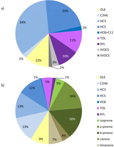
Our anthropogenic case study is based on the atmosphere in and near Mexico City during the MILAGRO (Megacity Ini-tiative: Local and Global Research Observations) campaign of March 2006 (Molina et al., 2010). The emissions and initial conditions are defined similar to L-T11, and briefly summarized here. Anthropogenic emissions are a mixture of light aromatics (21 % by mass), linear alkanes to C30 (44 % by mass, excluding CH4), a selection of branched alkanes to C8 (20 % by mass), and alkenes to C6 (12 % by mass) (see Fig. 1a). Diel cycles of emission rates of chem-ically similar groups with up to 10 carbons are specified following Tie et al. (2009). Emissions rates of individual species within the groups are specified according to their ob-served relative abundances (Apel et al., 2010). Long-chain n-alkanes are used as surrogates for all emitted semi-volatile and intermediate-volatility organic compounds (SVOCs and IVOCs). Their emitted masses are distributed among prede-fined volatility bins as described in L-T11. The NAN scheme yields vapor pressures that are progressively higher with increasing carbon number than are those given by JRMY. Hence, the emissions distribution of individual S/IVOCs re-quired to represent the same volatility distribution differs be-tween the two schemes, and was therefore recalculated for NAN in this study. The ninth and lowest volatility bin in the emissions (“SVOC1”, centered on C∗=1×10⁻²µg m−3, where C∗ is the effective saturation concentration)
12% 2%
34%
23%
2%
11%
10%
3% 2%
OLE
C2H6
HC3
HC5
HC8+C11
TOL
XYL
IVOCS
SVOCS
a)
9% 13% 13%
12% 1%
5%
1%
5%
16%
16%
4% 7%
OLE
C2H6
HC3
HC5
HC8
TOL
XYL
isoprene
a-pinene
b-pinene
carene
limonene
b)
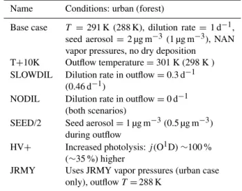
Figure 1.Precursor NMHC mass distributions for the outflow sim-ulation runs.(a)Urban case emissions by mass. Total emissions are 2.6 g m−2d−1. Species classes correspond loosely to those of the RACM mechanism (Stockwell et al., 1997) and the volatility-based nomenclature of Donahue et al. (2009). “OLE”, olefins; “C2H6”, ethane; “HC3”, propane and similar species; “HC5”,n-pentane and similar species; “HC8+C11”,n-alkanes with 8 to 11 carbons, and cyclohexane; “TOL”, toluene, benzene, and ethyl benzene; “XYL”, xylenes, trimethyl benzenes, and ethyl toluene; “IVOCS”,n-alkanes with 12 to 17 carbons; “SVOCS”,n-alkanes with 18 to 30 carbons. Branched alkanes constitute 16 and 66 % of the mass in classes “HC3” and “HC5”, respectively.(b)Forest case precursor inputs. Species classes are as in(a). Inputs shown total 0.23 g m−2d−1. In-puts of oxygenated C1–4 species are omitted for clarity, and com-prise an additional 0.7 g m−2d−1 including 0.2 g m−2d−1 from methyl vinyl ketone and methyl butenol, combined.
2.2.2 Forest precursors: Manitou Forest during BEACHON
Our biogenic case study is based on Manitou Forest dur-ing the BEACHON-ROCS field campaign of summer 2010 (Ortega et al., 2014). The site is dominated by ponderosa pine, giving an ambient VOC mixture high in monoterpenes and low in typical anthropogenic VOCs such as aromatics, alkanes, and alkenes. Emissions are represented via mixing-in of air with specified precursor concentrations based on observations (Kaser et al., 2013b). The precursor mix in-cludes selected monoterpenes (α- andβ-pinene at 0.11 ppbv
each, limonene at 49 pptv, and carene at 29 pptv). Speci-fied oxygenated C1–4 species include methyl vinyl ketone at 0.25 ppbv and methyl butenol at 0.78 ppbv. Isoprene, alka-nes to C6, alkealka-nes to C5, and aromatics are also included, in the proportions shown in Fig. 1b. Our forest case precur-sor mixture omits sesquiterpenes because our model has not yet been tested for their complex chemistry. Sesquiterpenes would likely increase the quantity of SOA formed; how-ever we would not expect significant changes to the timing of downwind SOA formation. Like monoterpenes, sesquiter-penes have lifetimes of the order of an hour or less (Atkinson et al., 1990; Shu and Atkinson, 1995). Changing multiday formation rates would thus require the lifetimes and SOA yields of second- or higher generation sesquiterpene prod-ucts (Ng et al., 2006) to greatly exceed those for monoter-penes since sesquiterpene source fluxes are relatively low (of the order of 10 % or less of monoterpene fluxes during the BEACHON campaign; Kaser et al., 2013a).
2.3 Meteorological conditions and sensitivity studies Our box model simulations represent photochemical evolu-tion and aerosol condensaevolu-tion in an air parcel that is advected out of a source region and undergoes chemical processing during several days as part of an outflow plume. We initialize the model in the source region, in an Eulerian configuration with diurnally varying precursor emissions, boundary layer depth, and meteorological conditions. The spin-up period in the urban scenario is driven with meteorological boundary conditions representative of average conditions in Mexico City in March 2006, as in L-T11. For biogenic simulations, spin-up meteorological conditions were based on previous regional modeling studies (Cui et al., 2014). Ambient tem-peratures and boundary layer behavior were similar between the urban and biogenic cases. The spin-up phase lasts for just over 1.5 days, into the early afternoon of our “day 1”. The model simulation then converts into a Lagrangian or outflow period which continues for an additional 3 and 7 days in the forest and urban base cases, respectively. Emissions cease and the air parcel (model box) maintains a fixed volume and meteorology and is subject to continuing photochemistry and to dilution with background air. Outflow period meteorolog-ical conditions are discussed below.
background concentrations are equal; hence its relative con-tribution to the total aerosol mass increases with dilution.
For each scenario we perform several sensitivity studies which are initialized with the same Eulerian conditions but diverge at the beginning of the outflow period. Our “base case” simulations continue with constant temperatures of 291 and 288 K in the urban and forest scenarios, respectively, zero emissions, and a constant e-folding dilution ratekdilof 1 d−1. Outflow conditions begin at 2pm in the forest sce-nario. In the urban scenario, temperature becomes constant and emissions cease at 15:00, and the outflow phase begins at 16:00, whenkdilbecomes fixed.
In the real world, a plume’s dilution rates and air tem-peratures are likely to be heterogeneous, varying diurnally as well as with changing plume altitude. However the sen-sitivity of photochemistry and gas–particle partitioning in a detailed box model to individual environmental variables is most clearly explored by keeping these parameters constant, varying only one at a time. Warmer temperatures should shift the equilibrium towards the gas phase, potentially reducing particle-phase mass (e.g., if aerosol-forming chemical reac-tions are not temperature sensitive). Our simulation denoted “T+10K” explores the effect on aerosol mass of an outflow temperature increased by 10 K. Plume dilution might also be expected to lead to lower particle mass, since decreasing gas-phase concentrations shift condensation equilibria in favor of evaporation. Simulation “SLOWDIL” is constrained sim-ilarly to the base case, however with the outflow-period dilu-tion rate reduced to 0.3 d−1in the urban case and 0.46 d−1 in the forest case. Simulation “NODIL” uses no dilution at all. Another variable governing the direction of conden-sation equilibrium is the existing particle mass itself, as-suming that Raoult’s law applies (Pankow, 1994a). Simula-tion “SEED/2” reduces seed aerosol mass by 50 %, starting from the beginning of the outflow period. Most of our urban outflow simulations inadvertently employed photolysis rates
∼20 % lower than in L-T11. Rates of photochemical for-mation and transforfor-mation of condensable oxidized products scale with actinic flux, altering the particle mass formation rate. Boundary-layer aerosol pollution reduces actinic flux at the surface but enhances it aloft (Palancar et al., 2013). Sim-ulation “HV+” tests the sensitivity of the particle mass pro-duction to increased ambient actinic flux. Effectivej(O1D) in case HV+is about twice that in our urban base case, and about one-third greater than in our forest base case. Finally, simulation “JRMY” is similar to the base case, but with the JRMY vapor pressure scheme, with the S/IVOC emissions adjusted as described above, and with outflow temperatures of 288 K. This last sensitivity study was only performed for the urban case. Simulation conditions are summarized in Ta-ble 1.
Table 1.List of sensitivity simulations
Name Conditions: urban (forest)
Base case T =291 K (288 K), dilution rate= 1 d−1, seed aerosol=2 µg m−3 (1 µg m−3), NAN vapor pressures, no dry deposition
T+10K Outflow temperature=301 K (298 K ) SLOWDIL Dilution rate in outflow=0.3 d−1
(0.46 d−1)
NODIL Dilution rate in outflow=0 d−1 (both scenarios)
SEED/2 Seed aerosol=1 µg m−3(0.5 µg m−3) during outflow
HV+ Increased photolysis:j(O1D)∼100 % (∼35 %) higher
JRMY Uses JRMY vapor pressures (urban case only), outflowT=288 K
3 Results
3.1 Photochemical environment
The concentrations of key oxidants simulated within our ur-ban scenario source region have similar profiles to those shown in Fig. 3 of L-T11 for Mexico City (oxidants are plotted in Fig. S1 in the Supplement). Peak urban source re-gion concentrations are [OH]=3.2×10⁶molec cm−3, [O
3] =116 ppbv, and [NOx]=260 ppbv. These values represent highly polluted urban conditions, where [OH] is suppressed by high [NOx], and are within the range of observations (Dusanter et al., 2009). In the outflow, [OH] increases until stabilizing on day 5 at∼8.5×10⁶molec cm−3. Meanwhile, [NOx] drops rapidly to < 0.8 ppbv, and O3 also declines in response to dilution to∼60 ppbv. The forest case shows oxi-dant concentrations towards the high end of remote observa-tions (e.g., Wolfe et al., 2014): in the forest outflow [OH] is fairly constant at ∼8×10⁶molec cm−3, [O
3] decreases from 62 to 50 ppbv and NOxfalls to consistently low values (∼0.2 ppbv).
sce-nario has 30 % higher [OH] but largely unaffected [O3] and [NOx]. The urban scenario enhancements continue to high but not unprecedented (Rohrer et al., 2014) peak values of
∼17×106molec cm−3, indicating that case HV+provides a good test of the effects on particle mass formation of accel-erated gas-phase photochemistry. Sensitivity studies T+10K and SEED/2 have little or no effect on oxidant outflow con-centrations.
3.2 Organic aerosol mass production
Figure 2 shows the development of the condensed organic aerosol generated in our set of urban and pine-forest out-flow simulations. Lower panels show simulated concentra-tions and O / C atomic ratios. The spin-up period shows a strong diurnal cycle in response to diel variations in emis-sions, photolysis, and ventilation. Once the outflow period begins, particle-phase concentrations first peak in response to photochemistry then generally decline in response to dilu-tion. On day 2 (the first full day of outflow), concentrations show an additional photochemistry-induced increase super-imposed on the declining baseline, however by day 3 (the second full day of outflow), chemistry-induced concentration changes are barely discernible in either case.
To quantify the regional OA mass increase in the expand-ing plume, which is more relevant to net direct climate effects than is local concentration, we integrate the aerosol concen-trations over the entire outflow region. Following L-T11, we defined MtOA as the organic aerosol mass in a dispersed air parcel with original volume of 1 m3, expressed in units of µg initial m−3: M
tOA = et.kdil[OA]t, where t is time since the start of the outflow phase. [OA]t does not include the prescribed constant seed aerosol concentration. Contrary to the progressive decreases in downwind aerosol concentra-tions, MtOA increases throughout the simulation period, al-though the two base scenarios show very different production rate characteristics from each other. In our urban base case (Fig. 2a), MtOA increases from 6 µg initial m−3at the start of the outflow phase by 140 % (to∼14 µg initial m−3) in the first 24 h of outflow, and by a factor of > 4 (to 26.5 µg initial m−3) over 4 days. To assess the limits of this production, we con-tinued the simulation for a further 3 days. Particle mass in-creased asymptotically to a maximum of 28.4 µg initial m−3 after about a week. Our forest base case (Fig. 2b) also shows particle mass production, although at a far slower rate. MtOA begins the outflow phase at 0.8 µg m−3 and increases by ∼60 % (0.5 µg initial m−3) in the first 24 h of outflow. There-after, however, the production rate slows substantially with MtOA rising by only another 5 % (to 1.33 µg initial m−3) dur-ing the latter 2 days of the simulation.
Figure 2 also shows particle mass development for our sensitivity simulations. The largest differences in simu-lated aerosol plume mass are those produced by changing the vapor pressure scheme (performed for the urban case only). Even within the city, JRMY predicts 50 % more
mid-afternoon aerosol mass than NAN. Downwind, the JRMY case aerosol increases its mass excess over the NAN case, growing by more than a factor of 3 in 2 days before reach-ing an asymptote at about 30 µg initial m−3at the end of day 4, slightly sooner than in the NAN case. The initial primary aerosol concentrations are very similar between the two sim-ulations, reflecting the similar volatility distribution of the prescribed emissions. The mass differences arise during SOA production and may be explained by the large differences in estimatedPvapfor individual species under the two different methods. For example, estimated Pvap values for aromatic oxidation products are generally lower by 1–3 orders of mag-nitude under JRMY than under NAN. This allows JRMY to condense SOA with a lesser degree of substitution and at an earlier point in the oxidation process and explains both the early relatively rapid production in the JRMY case, and its earlier slowdown as the available gas-phase precursors be-come depleted. We discuss the chemical composition of the growing aerosol in more detail later. One should not read too much into the slightly higher ending mass of the JRMY aerosol, since this run used lower outflow temperatures. The main result here is that the predicted multiday nature of OA mass production is not unique to one particular vapor pres-sure scheme. The following discussion refers to simulations performed with the NAN scheme only.
The response of the aerosol production rate to environ-mental conditions is shown in Fig. 2. Particle mass in the out-flow plume is rather insensitive to seed aerosol amount, drop-ping by no more than 5 % when the seed aerosol is reduced by 50 % (runs “SEED/2”). Raising the ambient temperature by 10◦C (runs “T+10K”) lowers the condensed aerosol mass
by between 8 and 25 % relative to the base simulation. In-creasing the available sunlight (run “HV+”) speeds up ini-tial SOA production. The final condensed aerosol mass is unaffected in the forest scenario, but lower by 9 % in the ur-ban scenario, likely owing to increased photolytic removal of semi-volatile gases. In all these sensitivity cases, the aerosol mass reductions noted are insufficient to lead to net mass loss in either the urban or the forest scenario.
30 25 20 15 10 5 0 Dilution-adjusted mass, µ
g initial m
-3 JRMY base case NODIL SLOWDIL SEED/2 HV+ T+10K 15 10 5 0 [OA], µ g m -3 8 7 6 5 4 3 2 1 0 Time, days 0.6 0.4 0.2 0.0 O:C 1.0 0.8 0.6 0.4 0.2 0.0 [OA], µ g m -3 3 2 1 0 Time, days 1.0 0.8 0.6 0.4 0.2 0.0 O:C 1.4 1.2 1.0 0.8 0.6 0.4 0.2 0.0 Dilution-adjusted mass, µ
g initial m
-3 base case SLOWDIL NODIL SEED/2 HV+ T+10K a) b)
Figure 2.Simulated aerosol development for the(a)urban and(b)forest cases. Upper panels show plume-integrated mass during the outflow phase; lower panels show concentrations and O : C ratios for the model-generated aerosol fraction in the source regions and outflow phases. Grey shading indicates approximate nighttime periods.
0 0.1 0.2 0.3 0.4 0.5
-4 -2 0 2 4
d ilu ion -corr e cte d pa ric ul a te mas s, µ g i n i i al m -3 3 2.5 2 1.5 1 c) 0 5 10 15 20 25 30 35 40
-4 -2 0 2 4 6 8
d ilu ion -corr ecte d mass , µ g i niial m -3 b) 0 0.2 0.4 0.6 0.8 1 1.2 1.4 1.6 1.8 2
-4 -2 0 2 4 6 8
d il u ion -corr e cte d m ass , µ g iniial m -3
log10 (C*), µg m-3
d) 0 2 4 6 8 10
-4 -2 0 2 4
d il u ion -corr e cte d p ariculat e mas s, µ g ini ial m -3
log10 (C*), µg m-3
5 4 3 2 1 a)
log10 (C*), µg m-3
log10 (C*), µg m-3
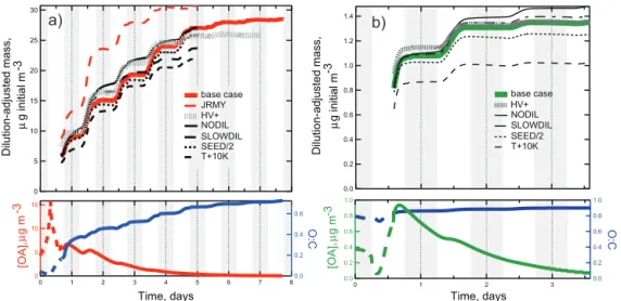
Figure 3.Time evolution of volatility distributions.(a, b)Urban case and(c, d)forest case. Solid lines, particle phase; dotted lines, gas phases. Colors represent different times (see key): whole numbers are midnight values (e.g., “1” is midnight between days 1 and 2), and half-day numbers are noon values (e.g., “1.5” is noon on day 2). The volatility continuums have been binned in decadal increments for ease of comparison with so-called volatility basis set (VBS) parameterizations.
mentioned in Sect. 3.1). It is likely coincidental that the com-binations of conditions in the NODIL and base cases lead to similar SOA mass production. From the point of view of our sensitivity study, however, the general result is that particle mass production integrated over the plume is only slightly sensitive to rather radical changes in the dilution rate. This shows that the SOA production is not an artifact of the nu-merical integration.
3.3 Particle-phase chemical composition and properties
to 0.42 after 24 h and 0.71 after 6 days, indicating a particle phase that becomes progressively more oxidized with time. Our forest model-generated OA fraction shows higher O : C ratios throughout (Fig. 2b, lower), developing from 0.84 to 0.90. The differences between the urban and forest scenar-ios are consistent with the forest case particle phase being already well oxidized at the beginning of the outflow phase, with delayed chemistry in the urban case outflow resulting from [OH] suppression, and with different precursor assem-blages giving differently oxidized products (e.g., Chhabra et al., 2011).
O : C values are highly sensitive to the aerosol fraction considered. Our simulations use a pre-existing seed aerosol with a mass concentration of 2(1) µg m−3in the urban (for-est) scenarios, respectively. We assign this seed aerosol the same O : C ratio as seen at the end of our forest case (0.9), consistent with a regional background aerosol that is well ox-idized and/or of largely biogenic origin (e.g., Hodzic et al., 2010). Including the seed aerosol raises calculated O : C to 0.35 (0.87) at the start of outflow in the urban (forest) cases. The seed aerosol contribution continues to influence the O : C ratio in the outflow, raising urban values to 0.55 after 24 h and 0.71 after 2.2 days (rather than 7 days). These values are comparable to measurements in Mexico City (0.4–0.73; Aiken et al., 2008; corrected as per Canagaratna et al., 2014), although the strong sensitivity of the O : C ratio to the back-ground aerosol means that model–measurement comparisons are of only limited utility if the background contribution is not known. Our forest scenario values are somewhat higher than measurements during the BEACHON campaign (gener-ally 0.5–0.77; Palm et al., 2013), suggesting that our model forest scenario has less anthropogenic influence than do the field data.
The chemical composition of organic aerosol may also be expressed in terms of the average molecular weight per car-bon (OM : OC), which includes the mass contributions of substituents such as nitrogen. Typical OM : OC values are 1.6±0.2 and 2.1±0.2 for urban and nonurban areas, respec-tively (Turpin and Lim, 2001). OM : OC for our modeled ur-ban outflow aerosol rises from 1.41 to 2.21 over 7 days, con-sistent with a progression from urban to nonurban regimes, while OM : OC in our forest outflow case rises only incre-mentally, from 2.25 to 2.32, in agreement with the published nonurban values.
Examining the evolution of volatility of the particle phase (Fig. 3) shows that particle composition is dynamic in both the urban and forest cases. The particles progressively lose molecules of higher volatility, and gain molecules with lower volatility. The details vary, but the net result is that particle-phase composition evolves, becoming less volatile with time. This is especially marked in the urban outflow scenario, where the envelope of the volatility distribution shifts to the left by 2 orders of magnitude.
Figure 4 investigates the molecular composition of the simulated particle phase, in terms of carbon number and
ex-0 0.1 0.2 0.3 0.4 0.5 0.6
4 6 8 10 12 14 16 18 20 22 24 26 28 30
di luti on -c or rec ted par ti c ul ate m as s , µ g ini ti al m -3 C# 5+ groups 4 groups 3 groups 2 groups 1 group 0 groups a) 0 0.5 1 1.5 2 2.5 3
4 6 8 10 12 14 16 18 20 22 24 26 28 30
d iluti on -c or rec ted par ti c ul ate m as s , µ g ini ti al m -3 C# c) 0 0.1 0.2 0.3 0.4 0.5 0.6 0.7 0.8
4 6 8 10
di luti on -c or rec ted par ti c ul ate m as s , µ g ini tal m -3 C# b) 0 0.1 0.2 0.3 0.4 0.5 0.6 0.7 0.8
4 6 8 10
di luti on -c orr ec ted parti c ul ate m as s , µ g ini ti al m -3 C# d)
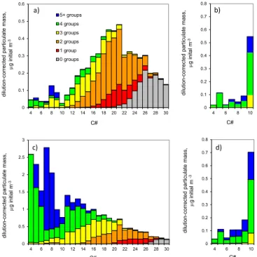
Figure 4.Particle mass composition binned by carbon number and number of functional groups per constituent molecule.(a)Urban case at start of outflow phase;(b) forest case at start of outflow phase;(c)urban case after 4 days;(d)forest case after 3 days.
pe-0 0.2 0.4 0.6 0.8 1 1.2
0 2 4 6 8 10 12
0 2 4 6 8
O
:C
raio
d
ilu
ion
-correcte
d
p
ar
icle
ph
as
e
mas
s,
µ
g
C i
nii
a
l m
-3
ime, days
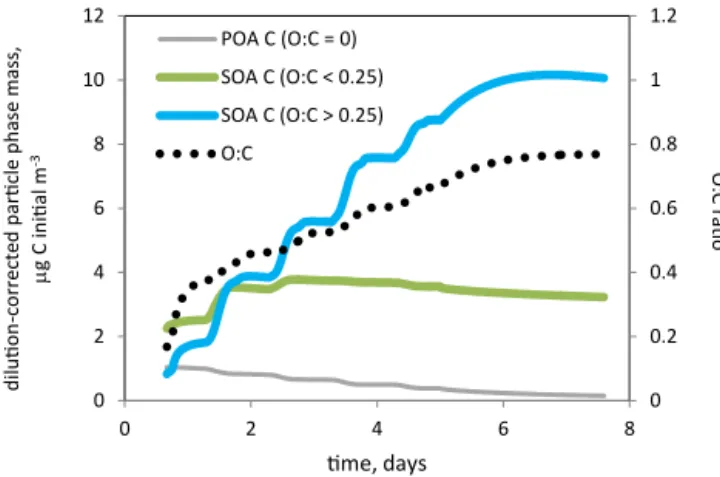
POA C (O:C = 0)
SOA C (O:C < 0.25)
SOA C (O:C > 0.25)
O:C
Figure 5.Evolution of the O : C ratio in the particle phase for the urban case. Left axis and solid lines: plume-integrated carbon mass of particle-phase fractions, segregated by O : C ratio. Right axis and black dotted line: O : C ratio of the entire particle phase.
riod (Fig. 4b), with most of the contributing species hav-ing ≥4 functional groups. Again, the particle phase adds more highly functionalized material during the outflow pe-riod (Fig. 4d) and loses small amounts of less-functionalized material. However, the compositional differences between the early- and late-stage particle phases are much less marked than in the urban case.
The long-term particle-phase production is much stronger in the urban outflow case than in the forest case; therefore we focus our attention on the urban case with the goal of identifying the compounds that are driving this production. We have already noted that O : C rises throughout the ur-ban outflow simulation. Figure 5 divides the carbon mass in the growing particle phase into fractions based on O : C ratio. The figure shows that the long-term particle mass pro-duction is entirely due to more-highly substituted material, with O : C > 0.25. Furthermore, and consistent with Fig. 4, mass-balance considerations show that the majority of this production cannot be explained by the sequence of evap-oration, oxidation (possibly including fragmentation), and recondensation of the less-substituted fractions, since these fractions show comparatively minor losses. The production must therefore be largely due to ongoing incorporation of previously uncondensed material from the gas phase.
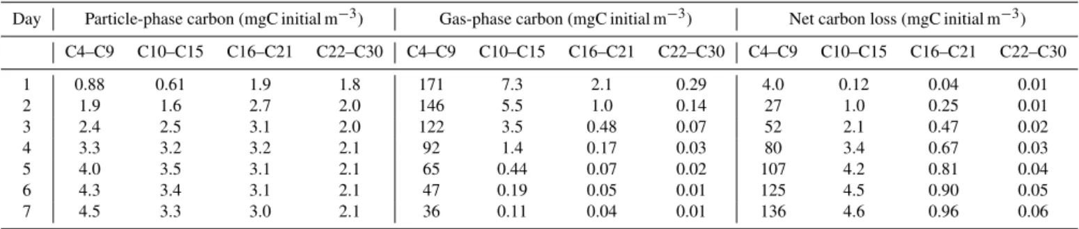
Figure 6 and Table 2 illustrate the temporal development of gas–particle partitioning for the urban case. The black lines in the figure represent the carbon mass in each C num-ber bin at the start of the outflow period, with the lower line representing the phase partitioning at that time between par-ticle (below the line) and gas (above the line). The colors of the sub-bars represent the partitioning after 4 outflow days. Brown shows particulate carbon, green shows gas-phase car-bon, and white shows the net carbon loss from each C num-ber bin during the outflow period. Carbon is conserved in our model (numerical losses are of the order of 0.1 % per
model day). The lost fraction in Fig. 6 and Table 2 represents fragmentation which reduces the C number of a molecule, moving carbon to the left and eventually off the figure into species with C number < 4. Some general trends are appar-ent. For the largest, least volatile molecules (C≥22), virtu-ally all the carbon partitions to the particle phase, either ini-tially or during the outflow period. Thus, further carbon mass production in this C number range is limited to small incre-ments from evaporation–oxidation–recondensation cycling. The gas-phase reservoir is also essentially depleted for the mid-sized molecules (with C number=10–21). However not all the carbon has partitioned into the particle phase, with a substantial portion (up to 60 %) removed by fragmentation. Some initial oxidation is usually necessary for fragmenta-tion to occur. The competifragmenta-tion between funcfragmenta-tionalizafragmenta-tion and fragmentation shifts in favor of increasing fragmentation for molecules with lower C number for two reasons. First, the branching ratio for CO2 elimination from peroxyacyl rad-icals increases with decreasing molecular length (Arey et al., 2001; Chacon-Madrid et al., 2010), and second, longer molecules generally have lower volatility and thus partition earlier to the particle phase, where they are protected from further gas-phase reaction (Aumont et al., 2012). For the smaller molecules (C number=4–9), fragmentation is the major fate, with only a few percent of the carbon in each bin becoming condensed. However, the much greater burden of these precursors in the outflow means that their contribu-tion to outflow SOA is comparable to that from the mid-sized molecules, and allows substantial particle mass production despite the significant losses to fragmentation. Furthermore, a gas-phase carbon reservoir persists in this size range, al-lowing the possibility of further particle mass production if sufficient functionalization can occur.
3.4 Chemical identity of species responsible for the production
The chemical composition of the gas–particle mixture can be explored in detail uniquely with GECKO-A, because it retains the explicit molecular identity of all intermediates and products. Figure 7 shows the time evolution of produc-tion rates for different chemical types within the urban out-flow particle phase. Production rates fluctuate diurnally in response to photochemistry, showing both a daytime max-imum corresponding to the solar-driven cycle in OH and a secondary production peak at sunset originating from nitrate radical chemistry. Mass losses (negative production) also have photochemically driven diurnal cycles, with aerosol constituents re-volatilizing in response to gas-phase removal. The particle phase shows production far exceeding losses for the most abundant individual secondary species and for most groups of similar species.
0 0.25 0.5 0.75 1 1.25 1.5
4 6 8 10 12 14 16 18 20 22 24 26 28 30
C#
net loss from bin
gas phase
paricle phase
iniial OA Carbon
iniial total carbon
0 10 20 30 40 50 60
4 5 6 7 8 9
d
il
u
i
o
n
-c
o
rr
ec
ted
c
ar
b
o
n
ma
ss
,
µ
g
C
in
i
i
a
l
m
-3
C#
Figure 6.Carbon partitioning budget during the urban outflow simulation. Black lines show the gas (dashed line) and particle (solid line) phases at the start of outflow. Stacked bars show partitioning after 4 days: brown, particle phase; light green, persisting gas phase; white, net loss to fragmentation. Carbon numbers 4 to 9 are plotted twice, on different scales, to allow the details of the partitioning to be seen more clearly.
Table 2.Carbon partitioning budget time series for the urban outflow simulation. Values are assessed at midnight on the days indicated. Losses are assessed relative to 16:00. on day 1. Values < 100 are rounded to either two significant figures or two decimal places.
Day Particle-phase carbon (mgC initial m−3) Gas-phase carbon (mgC initial m−3) Net carbon loss (mgC initial m−3)
C4–C9 C10–C15 C16–C21 C22–C30 C4–C9 C10–C15 C16–C21 C22–C30 C4–C9 C10–C15 C16–C21 C22–C30
1 0.88 0.61 1.9 1.8 171 7.3 2.1 0.29 4.0 0.12 0.04 0.01
2 1.9 1.6 2.7 2.0 146 5.5 1.0 0.14 27 1.0 0.25 0.01
3 2.4 2.5 3.1 2.0 122 3.5 0.48 0.07 52 2.1 0.47 0.02
4 3.3 3.2 3.2 2.1 92 1.4 0.17 0.03 80 3.4 0.67 0.03
5 4.0 3.5 3.1 2.1 65 0.44 0.07 0.02 107 4.2 0.81 0.04
6 4.3 3.4 3.1 2.1 47 0.19 0.05 0.01 125 4.5 0.90 0.05
7 4.5 3.3 3.0 2.1 36 0.11 0.04 0.01 136 4.6 0.96 0.06
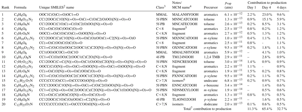
20 most abundant individual species (Table 3), three in par-ticular stand out. The fastest-growing single species dur-ing daytime is hydroxy-hydroperoxy-maleic anhydride, or “MALANHYOOH”. It is a major product of the oxida-tion of several different precursors including toluene andα -pinene, and its production rate is roughly correlated with the increasing trend in noontime [OH]. The chemical path-way involves unsaturatedγ-dicarbonyl fragmentation prod-ucts which recyclize to yield maleic anhydride and then un-dergo addition reactions with OH and HO2. This species ac-counts for about 7 % of the particle phase by the simula-tion end. The fastest-growing species at nightfall is “MN-NCATCOOH”, a post-aromatic fourth-generation oxidation product of toluene. It is a peroxide-bicyclic alkene (hereafter denoted “PBA”) with five functional groups: nitrate, nitro-and hydroperoxy, nitro-and two hydroxy groups. It arises from a sequence of oxidation reactions of toluene culminating in nitrate addition to nitro-di-hydroxy toluene (nitro-catechol), which breaks the aromaticity of the molecule. Its daytime analog, “MNCATECOOH”, is the nitro-hydroperoxide triol, and is the second-fastest-growing single species during
day-time. Together these three species make up 15 % of the parti-cle phase by the end of the simulation. They are also among the most abundant aerosol species in the forest case (Table 4) despite the low abundance of aromatic precursors.
four-Lee-T
aylor
et
al.:
Multiday
pr
oduction
of
condensing
or
ganic
aer
osol
mass
in
urban
and
for
est
outflo
w
605
Table 3.The top 20 contributors to modeled particle-phase production over the first 4 days1of the urban outflow simulation.
Notes/ pvap Contribution to production
Rank Formula Unique SMILES2name Class3 MCM name4 Precursor (atm) Day 1 Day 4 4 days
1 C4H4O6 OOC1C(O)C(=O)OC1=O MMAL MALANHYOOH aromatics 6.1×10⁻¹² 2.2 % 23.0 % 9.6 %
2 C7H8O11N2 CC12OOC(C1O[N](=O)=O)C(=C(O)C2(O)OO)[N](=O)=O 5f-PBN MNNCATCOOH toluene 1.3×10⁻¹³ 0.9 % 15.1 % 5.9 % 3 C7H9O9N CC12OOC(C1O)C(=C(O)C2(O)OO)[N](=O)=O 5f-PB MNCATECOOH toluene 2.6×10⁻¹³ 0.2 % 8.5 % 3.1 %
4 C5H8O6 CC(=O)C(O)C(OO)C(O)=O C < 8 fragment5 aromatics 2.5×10⁻¹¹ 0.8 % 0.2 % 1.2 %
5 C5H7O9N OOCC(=O)C(O)C(O)C(=O)OO[N](=O)=O C < 8,N fragment aromatics 2.7×10⁻¹² 0.5 % 1.3 % 1.2 %
6 C8H10O11N2 CC12OOC(C)(C1O[N](=O)=O)C(O)(OO)C(=C2[N](=O)=O)O 5f-PBN MXNNCATOOH m-xylene 1.0×10⁻¹³ 0.4 % 1.1 % 1.1 %
7 C5H8O6 CC(=O)C(OO)C(O)C(O)=O C < 8 fragment aromatics 2.5×10⁻¹¹ 0.8 % - 1.1 %
8 C8H10O11N2 CC1=C(O)C(O)(OO)C2(OOC1(C)C2O[N](=O)=O)[N](=O)=O 5f-PBN OXNNCATOOH o-xylene 9.5×10⁻¹⁴ 0.2 % 1.8 % 1.1 %
9 C5H6O6 CC1(OO)OCOC(=O)C1O MMAL MMALNHYOOH aromatics 5.9×10⁻¹² – 4.1 % 1.0 %
10 C8H11O8N CC1=CC(O)(OO)C2(OOC1(C)C2O)[N](=O)=O 4f-PB TM124NOOH 1,2,4 TMB 2.9×10⁻¹¹ – 2.8 % 0.9 %
11 C7H7O12N3 CC12OOC(C=C([N](=O)=O)C1(O)OO)(C2O[N](=O)=O)[N](=O)=O 5f-PBN NDNCRESOOH toluene 3.0×10⁻¹⁴ 1.4 % 0.9 % 0.9 % 12 C5H5O13N3 OOCC(C(O[N](=O)=O)C(=O)OO[N](=O)=O)C(=O)OO[N](=O)=O C < 8,N fragment aromatics 2.2×10⁻¹¹ 1.1 % - 0.9 %
13 C5H7O8N CC(=O)C(O[N](=O)=O)C(OO)C(O)=O C < 8,N fragment aromatics 1.9×10⁻¹¹ 1.5 % 0.2 % 0.8 %
14 C8H10O11N2 CC1=C(O)C(O)(OO)C2(C)OOC1(C2O[N](=O)=O)[N](=O)=O 5f-PBN PXNNCATOOH p-xylene 9.5×10⁻¹⁴ 0.2 % 1.1 % 0.7 % 15 C11H21O7N CCC(CCC(O)CC(=O)CCCOO)O[N](=O)=O C > 7,N isomers6 undecane 6.8×10⁻¹³ 0.2 % 0.9 % 0.7 % 16 C8H10O11N2 CCC12OOC(C1O[N](=O)=O)C(=C(O)C2(O)OO)[N](=O)=O 5f-PBN ENNCATCOOH e-benzene 3.4×10⁻¹⁴ – 1.4 % 0.6 % 17 C8H9O12N3 CC1=C([N](=O)=O)C2(OOC(C)(C2O[N](=O)=O)C1(O)OO)[N](=O)=O 5f-PBN NDNMXYLOOH m-xylene 1.9×10⁻¹⁴ – 0.5 % 0.6 % 18 C6H9O8N CC(=O)C(C)(OO)C(O[N](=O)=O)C(O)=O C < 8,N fragment aromatics 1.3×10⁻¹¹ 0.8 % 0.3 % 0.5 %
19 C7H9O8N CC12OOC(C1O)C(O)(OO)C(=C2)[N](=O)=O 4f-PB TL4ONO2OOH p-xylene 2.2×10⁻¹¹ – 1.6 % 0.5 %
20 C12H23O7N CCCC(CCC(O)CC(=O)CCCOO)O[N](=O)=O C > 7,N isomers dodecane 2.0×10⁻¹³ 0.1 % 0.6 % 0.5 % Total7contribution to production 11.3 % 65.4 % 32.7 %
1Days as used in this table are 24 h periods beginning at 16:00
2Unique SMILES notation is based on the original definition of Weininger (1988) and referenced online at http://cactus.nci.nih.gov/translate/, February 2014.
3Class names are defined in the text.
4MCM names follow the notation of Jenkin et al. (2003) and Bloss et al. (2005b), as referenced online at http://mcm.leeds.ac.uk/MCM, February 2014.
5Fragmentation products shown here all have several different aromatic precursors.
6Isomer lumping protocol is described by Valorso et al. (2011) and Aumont et al. (2008).
7The remainder consists of species whose individual contributions are not in the top 20.
.atmos-chem-ph
ys.net/15/595/2015/
Atmos.
Chem.
Ph
ys.,
15,
595–
615
,
-0.2 -0.1 0 0.1 0.2 0.3 0.4
0 1 2 3 4 5 6 7 8
d
il
u
ti
on
-c
or
rec
ted
p
rod
u
ct
ion
r
a
te,
m
g
h
ou
r
-1 in
it
ial
m
-3
Time (days)
zero
aromatics
(M)MAL
5f-PBN
5+4f-PB
others a)
-0.2 -0.1 0 0.1 0.2 0.3 0.4
0 1 2 3 4 5 6 7 8
d
il
u
ti
on
-c
or
re
ct
e
d
p
rod
u
ct
ion
r
a
te
,
m
g
h
ou
r
-1 in
it
ial
m
-3
Time (days)
zero
POA
C<8,N
C<8,noN
C>7,N
C>7,noN b)
Figure 7.Hourly production rates of all species in the urban case particle phase, aggregated by broad chemical characteristics.(a)Cyclic products of aromatic precursors;(b)all other species. Colors show species groupings. See text for details.
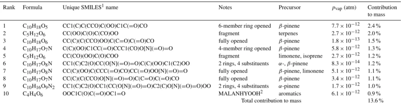
Table 4.The top 10 contributors to modeled particle mass at the end of the forest outflow simulation.
Rank Formula Unique SMILES1name Notes Precursor pvap(atm) Contribution
to mass
1 C10H18O5 CC1(C)C(CCO)C(OO)C1C(=O)CO 6-member ring opened β-pinene 7.7×10⁻¹² 2.4 %
2 C5H12O6 CC(OO)C(O)C(CO)OO fragment terpenes 2.7×10⁻¹² 2.0 %
3 C10H18O6 CC(C)(C(CCO)OO)C(C=O)C(=O)CO fully opened β-pinene 1.8×10⁻¹³ 1.5 %
4 C10H17O7N C(C)(OO)C1CC(=O)CCC1(CO)O[N](=O)=O 4-member ring opened β-pinene 5.8×10⁻¹² 1.3 %
5 C5H12O6 CC(CO)(OO)C(O)COO fragment limonene, isoprene 2.7×10⁻¹² 1.2 %
6 C10H17O8N CC1(C)C2(O)CC(O[N](=O)=O)C(C)(OO)C1(C2)OO 2 rings, 4 substituents α-,β-pinene 8.3×10⁻¹⁴ 1.2 %
7 C10H17O8N CC(C)(OO)C(CCC(=O)CO)CC(=O)OO[N](=O)=O fully opened β-pinene, limonene 5.1×10⁻¹² 1.1 %
8 C10H17O7N CC(C)(C(CCO)O[N](=O)=O)C(C=O)C(=O)CO fully opened β-pinene 3.4×10⁻¹² 1.1 %
9 C10H16O9N2 CC1(C)C2(O)CC1(CC(O[N](=O)=O)C2(C)O[N](=O)=O)OO 2 rings, 4 substituents α-pinene 1.7×10⁻¹² 1.0 %
10 C4H4O6 OOC1C(O)C(=O)OC1=O MALANHYOOH2 aromatics 6.1×10⁻¹² 0.9 %
Total contribution to mass 13.6 %
1Unique SMILES notation; see Table 2.
2MCM name, as in Table 2.
functional PBAs. (The mechanism contains no nitrated four-functional PBAs.) These two classes also include a minor contribution (< 10 %) from di-nitro PBAs formed via di-nitro cresols. Together, the three classes (M)MAL, 5f-PBN and 5+4f-PB account for∼30 % of the aerosol mass production during the first 4 days of the urban outflow simulation, and
∼40 % over 7 days. Furthermore, their relative mass con-tributions start small ( < 5 % of aerosol mass) but become progressively greater, reaching∼25 % of aerosol mass in 4 days and ∼30 % in 7 days. Other ring-retaining products play little role. Class “aromatics” represents all species re-taining aromaticity, including substituted cresols and cate-chols, which are formed on day 1 but show small net losses from the particle phase over the first 4 days of outflow
0 1 2 3 4 5 6 7 8
-4 -3 -2 -1 0 1 2
d
ilu
i
o
n
-cor
re
cted
pariculate
mass
µ
g
in
ii
a
l
m
-3
log10(C*), µg m-3
4f-PB
5f-PB
5f-PBN
sub-arom
(M)MAL
C>7
C<8
all species
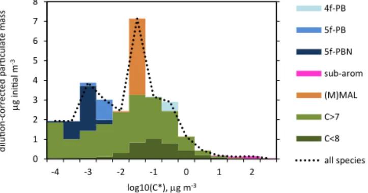
Figure 8.Chemical composition of the particle phase at the end of the urban outflow simulation, distributed by volatility. Colors show species groupings as discussed in the text: “C < 8” and “C > 7”, lin-ear/branched molecules separated by carbon number (no distinc-tion for nitrate is made here); “(M)MAL”, substituted maleic an-hydrides; “sub-arom”, substituted rings that retain aromaticity; “5f-PBN”, PBAs with five-functional groups including nitrate; “5f-PB”, as 5f-PBN without nitrate; “4f-PB”, PBAs with four-functional groups. Dotted line shows total particle-phase mass. The leftmost bin also includes the mass from species with log10(C∗) <−4.
and C > 7 noN contribute 33 % and 17 %, respectively, to net mass production, while classes C < 8 N and C < 8 noN contribute 16 % and 5 %, respectively. Production rates are strong for several days, mainly slowing to zero on or around day 5, with nitrated species showing more sustained pro-duction. The larger molecules (C > 7) are products of oxi-dation reactions of aliphatic compounds. Of these, C11–C13 species have the most rapid particle-phase production rates. The smaller molecules (C < 8) are products of sequential oxidation and fragmentation reactions of aromatic precur-sors, with C5 species contributing the most production. In terms of chemical identity, the species in these four classes are highly diverse, usually containing at least three differ-ent functional groups. Most C < 8 species with significant production contributions contain at least one PAN or car-boxylic acid group, resulting from oxidative addition to a double bond. This is not the case for the major C > 7 con-tributors, many of which contain δ-dicarbonyl, δ -hydroxy-hydroperoxy, and/orδ-hydroxy-ketone groups resulting from 1,5-hydrogen migration in alkoxy radicals (Orlando et al., 2003). In addition to the daytime production, C < 8N species show sustained nighttime production from nitrate and peroxy chemistry.
The chemical composition of the urban case particle phase is reflected in the shape of its volatility distribution (Fig. 3a). Figure 8 distributes by half-decade in log10(C∗) the ma-jor chemical classes defined above at the end of the urban simulation. Linear and branched species (classes C > 7 and C < 8) give an approximately lognormal distribution with re-spect to log10 (C∗). Superimposed on this base are peaks attributable entirely to products of aromatic chemistry. The largest peak, around log10(C∗)= −1.5, is due to the two
sub-stituted maleic anhydrides in class (M)MAL. The secondary peak around log10(C∗)= −3 results from classes 5f-PB and 5f-PBN. Class 4f-PB is more volatile, giving a small shoulder at log10(C∗)≈ −0.5, while the substituted aromatics produce only a tiny bump in the distribution, around log10(C∗)=2.
The top 10 species in the forest particle phase are listed in Table 4. The biogenic precursors (α- andβ-pinene, and to a lesser extent limonene, isoprene, and carene) give rise to a large variety of condensable oxidation products, as shown by the small mass contributions of even the most abun-dant species. The maximum individual contribution is only 2.4 %, and the top 10 species together account for < 14 % of the particle mass. The forest case aerosol is highly diverse, with species having both four- and six-member rings as well as ring-opened species and fragmentation products. Every species listed contains at least one hydroperoxy group, re-flecting the HO2-dominant chemistry of this case study. Ni-trated species account for about one-third of the mass. The multigenerational product MALANHYOOH appears as the 10th most abundant aerosol species.
4 Discussion and conclusions
both our urban and forest cases, these losses are balanced by fresh condensation of other molecules and/or evaporation– oxidation–condensation processes so that the particle-phase volatility distribution shifts to lower vapor pressures and be-comes progressively less vulnerable to re-evaporation.
Particle-phase mass production in our urban simulation is attributable in roughly equal proportion to oxidation prod-ucts of light-aromatic and long-chain n-alkane precursors. Dodecane has been shown in laboratory photooxidation ex-periments to produce SOA with fourth- and higher gener-ation products under low-NOxconditions (Yee et al., 2012; Craven et al., 2012). These experiments were performed over relatively long timescales (up to 36 h) and yielded cumula-tive OH exposures up to about 1×10⁸molec cm−3h, simi-lar to the 3-day OH exposure experienced by our base case urban aerosol (∼1.5×10⁸molec cm−3h). The production in aerosol mass we predict from four- and five-functional prod-ucts of C11-C13 n-alkanes during the first half of our sim-ulation is therefore consistent with laboratory results. We use long-chainn-alkanes in this study as surrogates for the wealth of different alkane species emitted in anthropogenic situations (Isaacman et al., 2012; Fraser et al., 1997; Chan et al., 2013). This seems a reasonable approximation since n -alkanes have been shown in several laboratory studies (Lim and Ziemann, 2009a; Yee et al., 2013; Loza et al., 2014) to give SOA yields intermediate between those of branched and of cyclic alkanes, owing to differing OH reaction rates and to the increased (decreased) propensity of branched (cyclic) alkanes to undergo fragmentation. Our model reproduces this behavior (Aumont et al., 2013). Using a more diverse anthro-pogenic precursor mix from that assumed here could alter the modeled particle-phase production rates and resulting mass, in either direction, but is unlikely to eliminate the production. Therefore these qualifications do not detract from our central result that the particle phase continues to grow for several days downwind of the urban source.
We have identified two specific classes of oxidation prod-ucts of light aromatics, the substituted maleic anhydrides and five-functional peroxide-bicyclic alkenes (including those with and without nitrate), as major contributors to the SOA production especially in the later days of the simulation. Their delayed influence in the evolving urban outflow is con-sistent with greater SOA yields from aromatic species under low-NOxconditions as observed by Chan et al. (2009) and Ng et al. (2007). In the present urban outflow study, these multigenerational products together contribute roughly 30 % of the particle-phase production. Admittedly, our calcula-tions use the NAN vapor pressure scheme far beyond the list of species for which it was validated. However, even if their vapor pressures are underestimated by 1–2 orders of magni-tude, these products should be sufficiently involatile to parti-tion strongly to the particle phase (see Fig. 7). We suggest that the substituted maleic anhydrides and five-functional peroxide-bicyclic alkenes might be useful targets for obser-vational studies seeking to validate our prediction of
multi-day anthropogenic aerosol production. The fact that only a few species classes contribute such a large proportion of our predicted particle mass production also affects the volatil-ity distribution of the developing aerosol, so that it deviates from a simple lognormal shape. If it can be shown that these species types are indeed important contributors to regional anthropogenic-origin SOA, it will be important to parame-terize their volatility distributions for inclusion in regional and global models of aerosol development.
Parameterizing SOA formation for routine modeling use is a complex task, and beyond the scope of this paper. Our re-sults can, however, offer some insight. First, and as might be expected, our results illustrate that biogenic, aliphatic anthropogenic, and light-aromatic anthropogenic SOA pre-cursors may be regarded as three distinct classes based on the timescales of resulting SOA mass development and the shapes of the product vapor pressure distributions. Within each of these broad groupings, there is considerable vari-ability of product volatility and chemical characteristics, and GECKO-A has already been used to parameterize correla-tions for use in 3-D models, e.g., between effective Henry’s law constant and volatility (Hodzic et al., 2013, 2014), be-tween volatility and mean oxidation state (Aumont et al., 2012), and between carbon number and polarity (Chung et al., 2012). The specific insights given by these studies should contribute to mechanism parameterization efforts.
In this study we do not address loss processes that could affect the particle mass in a plume. Explicit chemistry simu-lations have found dry deposition to be more important than wet deposition (Hodzic et al., 2014). Dry deposition reduces anthropogenic-origin SOA by 15–40 % and biogenic-origin SOA by 40–60 % over regionally relevant timescales, and depending on model conditions and assumed boundary layer depth (Hodzic et al., 2013, Hodzic et al., 2014). Other pos-sible conversion processes include in-particle accretion reac-tions (Barsanti and Pankow, 2004), heterogeneous oxidation (George and Abbatt, 2010a; Smith et al., 2009; Molina et al., 2004), photolysis (Nizkorodov et al., 2004), and multiphase chemistry (Pun and Seigneur, 2007; Ervens and Volkamer, 2010; Lim and Ziemann, 2009b). These processes, which be-come increasingly important at longer timescales, could ei-ther increase or decrease particle mass and could affect parti-cle hygroscopicity (e.g., George and Abbatt 2010b), and will also likely increase the SOA O : C ratio (e.g., Heald et al., 2010).
as-sumption that these OA are purely scattering in the short-wave spectrum, with RF per unit mass comparable to that of sulfate aerosols. Our results, on the other hand, suggest a much larger regional contribution from SOA of urban origin, specifically from the use of fossil fuels comprised in large part of aromatics and long-chain alkanes. The remarkable production shown in Fig. 2a would lead to a much larger anthropogenic contribution to the regional – and possibly global – burden of SOA, and their associated RF.
A crude estimate shows that large increases in anthro-pogenic SOA are plausible when viewed together with long-term anthropogenically driven increases in tropospheric ozone. Northern Hemisphere tropospheric background ozone has increased from preindustrial values around 10 ppb (Volz and Kley, 1988) to 30–40 ppb (Oltmans et al., 2013). While their precise precursors and formation/removal pathways dif-fer, both tropospheric O3 and SOA are byproducts of the NOx-catalyzed photooxidation of hydrocarbons, and are in-deed highly correlated in urban observations. Examples of correlation slopes vary from 30 µg m−3ppm−1 in Houston to 160 µg m−3ppm−1 in Mexico City (e.g., Wood et al., 2010), and application of these slopes to the Northern Hemi-sphere industrial-era increase in background O3would cor-respond to background SOA concentration increases of 0.6– 3.2 µg m−3. A simple extrapolation over the entire North-ern Hemisphere in a 1 km PBL implies a hemispheric bur-den of 0.15–0.8 Tg, and, assuming a 10-day lifetime (e.g., Kristiansen et al., 2012), an annual production rate of 5– 30 Tg yr−1. Thus it is evident that regional SOA of urban ori-gin has a large potential to modify RF on much larger scales. Unfortunately the optical properties of these SOA particles remain largely unknown; empirical evidence is mounting for strong absorption in the near UV (Kanakidou et al., 2005; Barnard et al., 2008; Lambe et al., 2013) and possibly visi-ble wavelengths as particles age (Updyke et al., 2012), con-sistent with the presence of complex chromophores such as conjugated carbonyls formed by particle-phase oligomeriza-tion (which is not currently represented in our model). The combined uncertainties from the regional production and op-tical properties of anthropogenic SOA cast some doubt on their current representation in global models.
We note also that, in contrast to the anthropogenic SOA, biogenic SOA does not seem to show strong multiday re-gional production. Given that biogenics represent over 90 % of global VOC emissions, even moderate production would have had a large impact on the total SOA budget and would likely yield unrealistically high global SOA concentrations. Anthropogenic VOCs, on the other hand, are shown by our study to have a potentially much larger sphere of influence than previously suspected. Of course we acknowledge many assumptions and approximations inherent in our study, and so we put forward our conclusions tentatively and semi-quantitatively, but with a hopefully clear message that further study is urgently needed to resolve these issues and increase
confidence in our understanding of how humans are affecting Earth’s climate.
The Supplement related to this article is available online at doi:10.5194/acp-15-595-2015-supplement.
Author contributions. J. Lee-Taylor, S. Madronich, and A. Hodzic
designed the study. J. Lee-Taylor and A. Hodzic performed the sim-ulations. All co-authors contributed to model development. J. Lee-Taylor prepared the manuscript with contributions from all co-authors.
Acknowledgements. The National Center for Atmospheric
Re-search is operated by UCAR and sponsored by the National Science Foundation. J. Lee-Taylor was supported by a grant from the US Department of Energy (Office of Science, BER, no. DE-SC0006780), which also partly supported S. Madronich. B. Aumont acknowledges support from the Primequal program of the French Ministry of Ecology, Sustainable Development and Energy; the Sustainable Development Research Network (DIM-R2DS) of the Ile-de-France region; and the French ANR within the project ONCEM.
Edited by: K. Tsigaridis
References
Aiken, A. C., DeCarlo, P. F., Kroll, J. H., Worsnop, D. R., Huff-man, J. A., Docherty, K. S., Ulbrich, I. M., Mohr, C., Kimmel, J. R., Sueper, D., Sun, Y., Zhang, Q., Trimborn, A., Northway, M., Ziemann, P. J., Canagaratna, M. R., Onasch, T. B., Alfarra, M. R., Prevot, A. S. H., Dommen, J., Duplissy, J., Metzger, A., Bal-tensperger, U., and Jimenez, J. L.: O / C and OM / OC ratios of primary, secondary, and ambient organic aerosols with highres-olution time-of-flight aerosol mass spectrometry, Environ. Sci. Technol., 42, 4478–4485, doi:10.1021/es703009q, 2008. Apel, E. C., Emmons, L. K., Karl, T., Flocke, F., Hills, A. J.,
Madronich, S., Lee-Taylor, J., Fried, A., Weibring, P., Walega, J., Richter, D., Tie, X., Mauldin, L., Campos, T., Weinheimer, A., Knapp, D., Sive, B., Kleinman, L., Springston, S., Zaveri, R., Or-tega, J., Voss, P., Blake, D., Baker, A., Warneke, C., Welsh-Bon, D., de Gouw, J., Zheng, J., Zhang, R., Rudolph, J., Junkermann, W., and Riemer, D. D.: Chemical evolution of volatile organic compounds in the outflow of the Mexico City Metropolitan area, Atmos. Chem. Phys., 10, 2353–2375, doi:10.5194/acp-10-2353-2010, 2010.
Aumont, B., Szopa, S., and Madronich, S.: Modelling the evolution of organic carbon during its gas-phase tropospheric oxidation: development of an explicit model based on a self generating ap-proach, Atmos. Chem. Phys., 5, 2497–2517, doi:10.5194/acp-5-2497-2005, 2005.
Aumont, B., Camredon, M., Valorso, R., Lee-Taylor, J., and Madronich, S.: Development of systematic reduction techniques to describe the SOA/VOC/NOx/O3 system, Atmospheric Chem-ical Mechanisms Conference, 2008.
Aumont, B., Valorso, R., Mouchel-Vallon, C., Camredon, M., Lee-Taylor, J., and Madronich, S.: Modeling SOA formation from the oxidation of intermediate volatilityn-alkanes, Atmos. Chem. Phys., 12, 7577–7589, doi:10.5194/acp-12-7577-2012, 2012. Aumont, B., Camredon, M., Mouchel-Vallon, C., La, S.,
Ouze-bidour, F., Valorso, R., Lee-Taylor, J., and Madronich, S.: Mod-eling the influence of alkane molecular structure on secondary organic aerosol formation, Faraday Discuss., 165, 105–122, doi:10.1039/c3fd00029j, 2013.
Baker, J., Arey, J., and Atkinson, R.: Rate constants for the gas-phase reactions of OH radicalswith a series of hydrox-yaldehydes at 296±2 K, J. Phys. Chem. A, 108, 7032–7037, doi:10.1021/jp048979o, 2004.
Barley, M. H. and McFiggans, G.: The critical assessment of vapour pressure estimation methods for use in modelling the formation of atmospheric organic aerosol, Atmos. Chem. Phys., 10, 749– 767, doi:10.5194/acp-10-749-2010, 2010.
Barnard, J. C., Volkamer, R., and Kassianov, E. I.: Estimation of the mass absorption cross section of the organic carbon component of aerosols in the Mexico City Metropolitan Area, Atmos. Chem. Phys., 8, 6665–6679, doi:10.5194/acp-8-6665-2008, 2008. Barsanti, K. C. and Pankow, J. F.: Thermodynamics of the
forma-tion of atmospheric organic particulate matter by accreforma-tion re-actions – Part 1: aldehydes and ketones, Atmos. Environ., 38, 4371–4382, doi:10.1016/j.atmosenv.2004.03.035, 2004. Barsanti, K. C., Carlton, A. G., and Chung, S. H.: Analyzing
exper-imental data and model parameters: implications for predictions of SOA using chemical transport models, Atmos. Chem. Phys., 13, 12073–12088, doi:10.5194/acp-13-12073-2013, 2013. Bloss, C., Wagner, V., Bonzanini, A., Jenkin, M. E., Wirtz, K.,
Martin-Reviejo, M., and Pilling, M. J.: Evaluation of detailed aromatic mechanisms (MCMv3 and MCMv3.1) against envi-ronmental chamber data, Atmos. Chem. Phys., 5, 623–639, doi:10.5194/acp-5-623-2005, 2005a.
Bloss, C., Wagner, V., Jenkin, M. E., Volkamer, R., Bloss, W. J., Lee, J. D., Heard, D. E., Wirtz, K., Martin-Reviejo, M., Rea, G., Wenger, J. C., and Pilling, M. J.: Development of a detailed chemical mechanism (MCMv3.1) for the atmospheric oxidation of aromatic hydrocarbons, Atmos. Chem. Phys., 5, 641–664, doi:10.5194/acp-5-641-2005, 2005b.
Boucher, O., Randall, D., Artaxo, P., Bretherton, C., Feingold, G., Forster, P., Kerminen, V.-M., Kondo, Y., Liao, H., Lohmann, U., Rasch, P., Satheesh, S. K., Sherwood, S., Stevens, B., and Zhan, X. Y.: Clouds and aerosols, in: Climate Change 2013: The Phys-ical Science Basis, Contribution of Working Group 1 to the Fifth Assessment Report of the IPCC, chap. 7, edited by: Stocker, T. F., Qin, D., Plattner, G.-K., Tignor, M., Allen, S. K., Boschung, J., Nauels, A., Xia, Y., Bex, V., and Midgley, P. M, Cambridge Uni-versity Press, Cambridge, UK, and New York, NY, USA, 571– 658, 2013.
Camredon, M., Aumont, B., Lee-Taylor, J., and Madronich, S.: The SOA/VOC/NOxsystem: an explicit model of secondary or-ganic aerosol formation, Atmos. Chem. Phys., 7, 5599–5610, doi:10.5194/acp-7-5599-2007, 2007.
Canagaratna, M. R., Jimenez, J. L., Kroll, J. H., Chen, Q., Kessler, S. H., Massoli, P., Hildebrandt Ruiz, L., Fortner, E., Williams, L. R., Wilson, K. R., Surratt, J. D., Donahue, N. M., Jayne, J. T., and Worsnop, D. R.: Elemental ratio measurements of or-ganic compounds using aerosol mass spectrometry: character-ization, improved calibration, and implications, Atmos. Chem. Phys. Discuss., 14, 19791–19835, doi:10.5194/acpd-14-19791-2014, 2014.
Carslaw, K. S., Lee, L. A., Reddington, C. L., Mann, G. W., and Pringle, K. J.: The magnitude and sources of uncer-tainty in global aerosol, Faraday Discuss., 165, 495–512, doi:10.1039/c3fd00043e, 2013.
Chacon-Madrid, H. J., Presto, A. A., and Donahue, N. M.: Function-alization vs. fragmentation:n-aldehyde oxidation mechanisms and secondary organic aerosol formation, Phys. Chem. Chem. Phys., 12, 13975–13982, doi:10.1039/c0cp00200c, 2010. Chan, A. W. H., Kautzman, K. E., Chhabra, P. S., Surratt, J. D.,
Chan, M. N., Crounse, J. D., Kürten, A., Wennberg, P. O., Flagan, R. C., and Seinfeld, J. H.: Secondary organic aerosol formation from photooxidation of naphthalene and alkylnaph-thalenes: implications for oxidation of intermediate volatility or-ganic compounds (IVOCs), Atmos. Chem. Phys., 9, 3049–3060, doi:10.5194/acp-9-3049-2009, 2009.
Chan, A. W. H., Isaacman, G., Wilson, K. R., Worton, D. R., Ruehl, C. R., Nah, T., Gentner, D. R., Dallmann, T. R., Kirchstetter, T. W., Harley, R. A., Gilman, J. B., Kuster, W. C., deGouw, J. A., Offenberg, J. H., Kleindienst, T. E., Lin, Y. H., Rubitschun, C. L., Surratt, J. D., Hayes, P. L., Jimenez, J. L., and Gold-stein, A. H.: Detailed chemical characterization of unresolved complex mixtures in atmospheric organics: insights into emis-sion sources, atmospheric processing, and secondary organic aerosol formation, J. Geophys. Res.-Atmos., 118, 6783–6796, doi:10.1002/jgrd.50533, 2013.
Chhabra, P. S., Ng, N. L., Canagaratna, M. R., Corrigan, A. L., Rus-sell, L. M., Worsnop, D. R., Flagan, R. C., and Seinfeld, J. H.: El-emental composition and oxidation of chamber organic aerosol, Atmos. Chem. Phys., 11, 8827-8845, doi:10.5194/acp-11-8827-2011, 2011.Craven, J. S., Yee, L. D., Ng, N. L., Canagaratna, M. R., Loza, C. L., Schilling, K. A., Yatavelli, R. L. N., Thornton, J. A., Ziemann, P. J., Flagan, R. C., and Seinfeld, J. H.: Analysis of secondary organic aerosol formation and aging using positive matrix factorization of high-resolution aerosol mass spectra: ap-plication to the dodecane low-NOxsystem, Atmos. Chem. Phys., 12, 11795–11817, doi:10.5194/acp-12-11795-2012, 2012. Chung, S. H., Lee-Taylor, J., Asher, W. E., Hodzic, A., Madronich,
S., Aumont, B., Pankow, J. F., and Barsanti, K. C., Develop-ment of a carbon number polarity grid secondary organic aerosol model with the use of Generator of Explicit Chemistry and Ki-netics of Organic in the Atmosphere, poster presented at AGU Fall Meeting, San Francisco, CA, 3–7 December, A53O–0368, 2012.