www.atmos-chem-phys.net/16/4343/2016/ doi:10.5194/acp-16-4343-2016
© Author(s) 2016. CC Attribution 3.0 License.
The vertical distribution of volcanic SO
2
plumes measured by IASI
Elisa Carboni1, Roy G. Grainger1, Tamsin A. Mather2, David M. Pyle2, Gareth E. Thomas3, Richard Siddans3, Andrew J. A. Smith4, Anu Dudhia4, Mariliza E. Koukouli5, and Dimitrios Balis5
1COMET, Atmospheric, Oceanic and Planetary Physics, University of Oxford, Clarendon Laboratory, Parks Road,
Oxford OX1 3PU, UK
2COMET, Department of Earth Science, University of Oxford, South Park Road, Oxford OX1 3AN, UK 3Rutherford Appleton Laboratory, Didcot, UK
4NCEO, Atmospheric, Oceanic and Planetary Physics, University of Oxford, Clarendon Laboratory, Parks Road,
Oxford OX1 3PU, UK
5Laboratory of Atmospheric Physics, Aristotle University of Thessaloniki, Thessaloniki, Greece
Correspondence to:Elisa Carboni ([email protected])
Received: 23 June 2015 – Published in Atmos. Chem. Phys. Discuss.: 11 September 2015 Revised: 7 March 2016 – Accepted: 14 March 2016 – Published: 7 April 2016
Abstract.Sulfur dioxide (SO2) is an important atmospheric
constituent that plays a crucial role in many atmospheric processes. Volcanic eruptions are a significant source of at-mospheric SO2 and its effects and lifetime depend on the
SO2injection altitude. The Infrared Atmospheric Sounding
Interferometer (IASI) on the METOP satellite can be used to study volcanic emission of SO2using high-spectral
reso-lution measurements from 1000 to 1200 and from 1300 to 1410 cm−1 (the 7.3 and 8.7 µm SO
2 bands) returning both
SO2amount and altitude data. The scheme described in
Car-boni et al. (2012) has been applied to measure volcanic SO2
amount and altitude for 14 explosive eruptions from 2008 to 2012. The work includes a comparison with the follow-ing independent measurements: (i) the SO2column amounts
from the 2010 Eyjafjallajökull plumes have been compared with Brewer ground measurements over Europe; (ii) the SO2plumes heights, for the 2010 Eyjafjallajökull and 2011
Grimsvötn eruptions, have been compared with CALIPSO backscatter profiles. The results of the comparisons show that IASI SO2measurements are not affected by underlying
cloud and are consistent (within the retrieved errors) with the other measurements. The series of analysed eruptions (2008 to 2012) show that the biggest emitter of volcanic SO2was
Nabro, followed by Kasatochi and Grímsvötn. Our observa-tions also show a tendency for volcanic SO2to reach the level
of the tropopause during many of the moderately explosive eruptions observed. For the eruptions observed, this tendency was independent of the maximum amount of SO2(e.g. 0.2 Tg
for Dalafilla compared with 1.6 Tg for Nabro) and of the vol-canic explosive index (between 3 and 5).
1 Introduction
Sulfur dioxide (SO2) is an important atmospheric
con-stituent, important in many atmospheric processes (Steven-son et al., 2003; Seinfeld and Pandis, 1998; Schmidt et al., 2012). Volcanic eruptions are a significant source of atmo-spheric SO2, with its effects and lifetime depending on the
SO2injection altitude. In the troposphere these include
acid-ification of rainfall, modacid-ification of cloud formation and im-pacts on air quality and vegetation (Ebmeier et al., 2014; Delmelle et al., 2002; Delmelle, 2003; Calabrese et al., 2011). In the stratosphere, SO2 oxidizes to form a
strato-spheric H2SO4 aerosol that can affect climate for several
years (Robock, 2000). Volcanoes contribute about one-third of the tropospheric sulfur burden (14±6 Tg S yr−1; Graf
et al., 1997; Textor et al., 2003). The annual amount of vol-canic SO2 emitted is both poorly constrained and highly
variable. The uncertainty in released SO2 arises from the
stochastic nature of volcanic processes, very little or no sur-face monitoring of many volcanoes, and from uncertainties in the contribution of volcanic sulfur emitted by quiescent (non-explosive) degassing. The effects of SO2in the atmosphere
at-4344 E. Carboni et al.: SO2vertical distribution of volcanic plumes
mospheric chemistry, as SO2 reactions and depletion times
change with height and atmospheric composition, particu-larly as a function of water vapour concentration (Kroll et al., 2015; von Glasow, 2010; McGonigle et al., 2004; Mather et al., 2003).
Most volcanic eruptions are accompanied by the release of SO2to the atmosphere, and data both on the quantity emitted,
and the height at which it is injected into the atmosphere are valuable indicators of the nature of the eruption.
It is important to monitor volcanic SO2 plumes for air
safety (Brenot et al., 2014; Schmidt et al., 2014) as sulfida-tion of nickel alloys cause rapid degenerasulfida-tion of an aircraft engine (Encinas-Oropesa et al., 2008). SO2is also used as
a proxy for the presence of volcanic ash, although the co-location of SO2and ash depends upon the eruption, so this
approach is not always reliable for hazard avoidance (Sears et al., 2013). Mitigation strategies to avoid volcanic SO2and
ash are currently based on ground monitoring and satellite measurements to assess the location and altitude of the prox-imal volcanic plume, followed by the use of dispersion mod-els to forecast the future position and concentration of the plume (Tupper and Wunderman, 2009; Bonadonna et al., 2012; Flemming and Inness, 2013). The outputs of the mod-els are strongly dependent on the assumed initial plume alti-tude mainly because of the variability of the wind fields with altitude. The dispersion models may use an ensemble of pos-sible initial altitudes to identify all places where the plume can potentially arrive. Hence improving the accuracy of the initial plume altitude reduces the uncertainty in the location of the transported volcanic SO2.
Limb viewing satellite instruments, such as the Michel-son Interferometer for Passive Atmospheric Sounding (MI-PAS) and the Microwave Limb Sounder (MLS), can estimate the vertical profile of SO2(Höpfner et al., 2013; Pumphrey
et al., 2014) in the upper troposphere and lower stratosphere (UTLS), but generally cannot observe in the lower tropo-sphere. Nadir measurements, by both spectrometers and ra-diometers, have been used to retrieve SO2column amounts,
assuming the altitude of the plume, e.g. the Total Ozone Monitoring Spectrometer (TOMS, Carn et al., 2003), the Moderate Resolution Imaging Spectroradiometer (MODIS, Watson et al., 2004; Corradini et al., 2009), the Ozone Mon-itoring Instrument (OMI, Krotkov et al., 2006; Yang et al., 2009; Carn et al., 2009), the Atmospheric Infrared Sounder (AIRS, Prata and Bernardo, 2007), the Advanced Spaceborne Thermal Emission and Reflection Radiometer (ASTER, Pug-naghi et al., 2006; Campion et al., 2010), the Global Ozone Monitoring Experiment 2 (GOME-2, Rix et al., 2012), and the Spinning Enhanced Visible and Infrared Imager (SE-VIRI, Prata and Kerkmann, 2007).
Nadir spectrometer measurements in the ultraviolet (OMI, GOME-2) and infrared (AIRS, the Tropospheric Emission Sounder, TES, IASI) can be used to infer information on the SO2plume altitude. This is based on the fact that the
top-of-atmosphere radiance of a plume, with the same amount
of SO2but at another altitude, will have a different spectral
shape within the SO2absorption bands.
UV spectra have been used to retrieve information on SO2
altitude by Nowlan et al. (2011) using an optimal estima-tion retrieval applied to GOME-2 measurements. Yang et al. (2010) used a direct fitting algorithm to retrieve the SO2
amount and altitude from OMI data. Both of these techniques were applied to the 2008 Kasatochi eruption which injected a relatively large amount of SO2high (circa 12 km) in to the
atmosphere. A new scheme to retrieve altitude from GOME-2 has been developed by Van Gent et al. (GOME-2016) and applied to Icelandic eruption case studies (Koukouli et al., 2014a).
Volcanic SO2 retrievals from satellite data in the thermal
infra-red (TIR) part of the spectrum are based on two regions of SO2absorption around 7.3 and 8.7 µm. The strongest SO2
band is at 7.3 µm. This is in a strong water vapour (H2O)
ab-sorption band and is not very sensitive to emission from the surface and lower atmosphere. Above the lower atmosphere this band contains information on the vertical profile of SO2.
Fortunately differences between the H2O and SO2emission
spectra allow the signals from the two gases to be decou-pled in high resolution measurements. The 8.7 µm absorption feature is in an atmospheric window so it contains informa-tion on SO2from throughout the column. In Clerbaux et al.
(2008) the SO2absorbing feature around 8.7 µm was used to
retrieve the total SO2amount and profile from TES data by
exploiting this instrument’s ability to resolve the change in SO2line-width with pressure. The 7.3 µm spectral range has
been used by Clarisse et al. (2014) in a fast retrieval of SO2
altitude and amount. Their approach, based on Walker et al. (2012), assumes that the SO2is located at different altitudes,
choosing the altitude that gives the best spectral fit.
In this paper, the Carboni et al. (2012) retrieval scheme (hereafter C12) has been applied to study the vertical dis-tribution of SO2 for the major eruptions during the period
2008–2012 and for some minor low tropospheric eruptions such as an Etna lava fountain.
The aims of this paper are to test the retrieved SO2amount
and altitude against other data sets (we used CALIPSO backscattering profile to test the altitudes and Brewer ground measurements for the column amounts) and to study the vol-canic plumes from different eruption types and in different locations.
2 IASI data
IASI is a Fourier transform spectrometer covering the spectral range 645–2760 cm−1(3.62 to 15.5 µm) with
spec-tral sampling of 0.25 cm−1and an apodized spectral
resolu-tion of 0.5 cm−1(Blumstein et al., 2004).
It has a nominal radiometric noise of 0.1–0.3 K in the SO2
spectral range considered, according to (Hilton et al., 2012). The field-of-view (FOV) consists of four circular foot-prints of 12 km diameter (at nadir) inside a square of 50 km×50 km, step-scanned across track (with 30 steps).
The swath is 2100 km wide and the instrument can nominally achieve global coverage in 12 hours.
Observations are co-located with the Advanced Very High Resolution Radiometer (AVHRR), providing complementary visible/near infrared measurements. IASI carries out nadir observation of the Earth simultaneously with the Global Ozone Monitoring Experiment (GOME-2) also on-board METOP. GOME-2 is a UV spectrometer measuring SO2in
the UV absorption band and is used for both Differential Op-tical Absorption Spectroscopy (DOAS) (Rix et al., 2012) and optimal estimation retrievals (Nowlan et al., 2011) of SO2.
More information about IASI can be found in Clerbaux et al. (2009). The IASI level 1c data (geolocated with apodized spectra) used here were obtained from both the British At-mospheric Data Centre (BADC) archive and EUMETSAT Unified Meteorological Archive Facility (UMARF) archive.
3 SO2retrieval scheme
The retrieval scheme follows C12 (Carboni et al., 2012) where the SO2 concentration is parametrized as a
Gaus-sian profile in pressure (with 100 mb spread). Using IASI measurements from 1000 to 1200 cm−1 and from 1300 to
1410 cm−1, an optimal estimation retrieval (Rodgers, 2000)
is employed to estimate the SO2column amount, the height
and spread of the SO2profile, and the surface skin
tempera-ture.
The forward model, based on the Radiative Transfer model for TOVS (RTTOV) (Saunders et al., 1999) but extended to include SO2explicitly, uses ECMWF temperatures
interpo-lated to the measurement time and location. The retrieval technique uses an error covariance matrix, based on a clima-tology of differences between the IASI measurements and SO2-free forward modelled spectra. Any differences not
re-lated to SO2 between IASI spectra and those simulated by
a forward model are included in the covariance matrix. Note that the SO2retrieval is not affected by underlying cloud. If
the SO2is within or below an ash or cloud layer, its signal
will be masked and the retrieval will underestimate the SO2
amount, in the case of ash this is indicated by a cost function value greater than 2.
The retrieval is performed for every pixel where the SO2
detection result is positive (Walker et al., 2011, 2012). The scheme iteratively fits the forward model (simulations) with the measurements, to seek a minimum of a cost function. The
solution, when the measurements do not contain enough in-formation to retrieve all the parameters in the state vector, is strongly affected by the assumed a priori values. When the SO2 amount decreases, the spectral information decreases,
and it is not possible to retrieve both SO2 amount and
alti-tude. This often happens at the edge of the plume. In this work we use 400±500 mb as the a priori value for plume
altitude and 0.5±100 DU for column amount. In addition,
only quality-controlled pixels are considered; these are val-ues where the minimization routine converges within 10 it-erations, the SO2 amount is positive, the plume pressure is
below 1000 mb and the cost function is less than 10. Rigorous error propagation, including the incorporation of forward model and forward model parameter error, is built into the system, providing quality control and error estimates on the retrieved state. Retrieved uncertainties increase with decreasing altitude, nevertheless it is possible to retrieve in-formation in the lower troposphere and monitor volcanic de-gassing. In the case of two or multiple SO2layers the forward
model assumption of a single Gaussian layer is a source of error (and this error is not included in the pixel by pixel er-ror estimate). In this case the retrieved altitude is an effective altitude between the two (or more) plume layers; in partic-ular the altitude will be the one that is radiatively closer to the measured spectra and the altitude will be the radiatively equivalent altitude.
The altitude of the SO2plume strongly modulates the
re-trieval error as the contrast between plume temperature and surface temperature is a critical factor. The error in SO2
amount decreases with an increase in plume altitude. Typi-cal uncertainties are 2 DU for a plume centred at 1.5 km and less than 1 DU for plumes above 3 km.
When using the result from this setting of the retrieval scheme, the following caveats should be considered:
1. The retrieval is valid for SO2column amounts less than
100 DU (limit used in the computation of RTTOV coef-ficients) and altitudes less than 20 km (due to the used Gaussian profile with 100 mb spread). For higher erup-tions one should use a thinner Gaussian profile, for col-umn amounts bigger than 100 DU new RTTOV coef-ficients will be needed. At present both of these condi-tions produce results that do not pass the quality control. 2. Quality control and orbit gaps can produce artefacts (see
Sect. 6).
3. Care should be taken when using the altitude to infer if a plume is above or below the tropopause. It is therefore desirable to combine or confirm these measurements us-ing other measurements. This is because there are alti-tudes with the same temperature above and below the tropopause, and the SO2signal could be similar.
4346 E. Carboni et al.: SO2vertical distribution of volcanic plumes
4. The global annual mean variability between real atmo-spheric profiles and ECMWF profiles is included in the error covariance matrix, and then propagated into the retrieval errors. However, we cannot exclude some ex-treme events where the difference between ECMWF profiles and the real profile is at the tail of the annual global statistical distribution. In this case, local and sea-sonal covariance matrices could be used. For the re-trievals presented here a global covariance matrix has been used, computed using days from all four seasons. 5. Volcanoes also emit water vapour. If this emission is
larger than the water vapour variability considered in the error covariance matrix, the results could be affected by errors that are not included in the output errors. Comparisons with the Universite libre de Bruxelles (ULB) IASI SO2 data set, as well as UV-Vis
instru-ments such as GOME2/MetOp-A and OMI/Aura, have been performed and are cited in the relevant eruptions sec-tions. We simply note here that for the Grímsvötn erup-tion our data were compared to the ULB IASI/MetOp-A SO2and the Belgian Institute for Space Aeronomy
(BIRA-IASB) GOME2/MetOp-A SO2 retrievals (Koukouli et al.,
2014b). The Etna continuous outflow measurement were compared with Istituto Nazionale di Geofisica e Vulcanolo-gia (INGV) MODIS/Terra, Rutherford Appleton Labora-tory (RAL) MODIS/Terra, ULB IASI/METOP-A, German Aerospace Center (DLR) GOME2/MetOpA and ground-based Flame network measurements (Spinetti et al., 2014) and finally the data from the Eyjafjallajökull eruptions, with the DLR GOME2/MetOpA, the BIRA OMI/Aura and the AIRS data (Carboni et al., 2012; Koukouli et al., 2014a). More recently, data for the Bárdarbunga eruption were com-pared with the BIRA-IASB OMI/Aura data (Schmidt et al., 2015).
4 Altitude comparison with CALIOP
Vertical profiles of aerosol and clouds are provided by NASA’s Cloud Aerosol Lidar with Orthogonal Polariza-tion instrument (CALIOP, Winker et al., 2009) carried on the CALIPSO satellite. CALIOP’s vertical/horizontal reso-lution is 0.06/1.0 km at altitudes between 8.2 and 20.2 km.
CALIPSO is part of the A-train with an equatorial overpass time of ∼13.30. CALIOP and IASI have coincident
mea-surements around ±70◦ latitude. Moving from this latitude
towards the equator causes the time difference between the two measurements to increase.
CALIOP backscatter profiles have been averaged (to 3 km along-track, 250 m vertical) and CALIOP observations of volcanic plumes have been identified using SEVIRI false colour images based on the infrared channel at 8.7, 11 and 12 µm (Thomas and Siddans, 2015). CALIOP is sensitive to aerosol and water droplets that scatter sunlight; in the
case of volcanic eruptions these aerosols are H2SO4and ash.
SEVIRI is sensitive to both ash and SO2 since its channel
around 8.7 µm is within the SO2absorption band.
The criteria used to define a coincidence between CALIOP and IASI pixels were the following: a distance of<100 km
and a time difference of<2 h. With these relatively strict
criteria, the selected coincident data are only from the Ice-landic Eyjafallajökull and Grimsvötn eruptions. For the other eruptions considered (Puyehue–Cordón Caulle, June 2011; Nabro, June 2011; Soufrière Hills, February 2010) the dif-ferences in acquisition time between the CALIOP and IASI measurements are more than 2 h. It may be possible to anal-yse these eruptions in the future by using the wind field to account for the movement of the plume with time.
Figure 1 shows the comparison between CALIOP and IASI for the Eyjafjallajökull plume on the 7 May 2010. This is the CALIOP track presented by Thomas and Prata (2011) in which they identify both ash and SO2plumes in the
south-ern part of the track (less than 55◦N)- and SO
2-only plumes
in the northern part of the track (the scattering feature around 5 km between 55 and 60◦N where the scattering signal is
possibly from H2SO4aerosol resulting from the oxidation of
volcanic SO2).
Ash and SO2 are not necessarily advected together
(Thomas and Prata, 2011; Sears et al., 2013), but in these case studies (Figs. 1–4), there is good agreement between IASI and the backscattering features within the IASI error bars. This may be due to the presence of H2SO4associated with
the SO2plume. An important aspect to note is that in nearly
all of the coincidences for the Eyjafallajökull case (with the exception of a few pixels on 14 May) the volcanic plume is above a lower meteorological cloud. This is identifiable as the scattering layer at around 1 km height in Fig. 1 and be-tween 1 and 4 km in Figs. 2 and 3. This comparison against CALIOP in the presence of water cloud confirms that the re-trieval is not affected by underlying cloud. This is because the variability that such a cloud introduces is represented by the error covariance matrix, which includes radiance differences between the clear forward model and cloudy IASI spectra. An accurate retrieval of altitude is also an important factor for the estimate of SO2amount; this is because the thermal
SO2signal can be up to 1 order of magnitude different
be-tween different altitudes. A good comparison of altitude with CALIPSO then gives confidence in both altitude and column amount.
Figure 4 shows the Grimsvötn plume at the beginning of the eruption. There is separation between the higher part of the plume (dominated by SO2) moving higher and spreading
north, and the lower part of the plume (dominated by ash, but still with some SO2associated with it) moving south-west. It
Figure 1.CALIOP/IASI coincidences for the Eyjafjallajökull plume on 7 May 2010 for overpasses within 2 h off each other. Top plot:
CALIOP backscatter profile with IASI over-plotted retrieval altitude (black stars) and error bar (black line); middle plot: the IASI SO2
amount and error bars corresponding to the altitude plotted above; bottom plots: map of IASI SO2amount (left) and altitude (right) with
CALIPSO track (black line) and identifying the IASI pixel plotted above with black stars.
5 Comparison with Brewer ground data
During the Eyjafjallajökull eruption in April and May 2010, the volcanic plume overpassed several European ground measurement stations equipped with Brewer instruments. Brewer instruments are UV spectrophotometers, principally dedicated to measuring the total ozone column but also capa-ble of determining total column SO2(Kerr et al., 1981).
Ex-traction of the SO2signal from the UV measurements is
per-formed as a second step after the ozone quantity retrieval due to the much lower SO2absorption feature strength (De Muer
and De Backer, 1992). Depending on the amount of at-mospheric SO2affecting the instruments, the Brewer
spec-trophotometer has been shown to be sensitive both to anthro-pogenic SO2loading in the lower troposphere (Zerefos et al.,
2000) as well as to an overpass of a volcanic plume, which produces a strong SO2 signal within the ozone absorption
bands. These ground-based measurements have lately been used in Rix et al. (2012) in a comparison with the GOME-2/METOP-A SO2 retrievals and in the validation work of
the European Space Agency (ESA) projects (SMASH and
SACS21) on the 2010 and 2011 Icelandic eruptions
(Kouk-ouli et al., 2014a). The World Ozone and Ultraviolet Radia-tion Data Centre (WOUDC) is an active archive facility that includes quality-assured Brewer ground-based O3
measure-ments and also provides SO2 daily averages. The data set
for April and May 2010 was downloaded from the WOUDC archive (http://www.woudc.org/) for all European sites with Brewer instruments.
The reported SO2amount in non-volcanic conditions (e.g.
over Europe before 15 April 2010) from Brewer stations varies considerably, which can mostly be attributed to the small signal-to-noise ratio of the SO2 signal compared to
the ozone signal. This variability may also be due to insuf-ficient reported data quality control with respect to SO2
re-trieval, since most stations focus on the quality of the ozone measurements and not their by-products. Negative values can also be present in the daily average data sets, a result of the nominal Brewer algorithm’s inability to resolve small atmo-spheric SO2amounts. Therefore, only a subset of the
avail-1“Study on an End-to-End system for volcanic ash plume
4348 E. Carboni et al.: SO2vertical distribution of volcanic plumes
4350 E. Carboni et al.: SO2vertical distribution of volcanic plumes
Figure 4.CALIOP/IASI coincidences for the Grímsvötn eruption on 22 and 23 May 2011. The blue arrow indicates the higher part of the
0 2 4 6 8 10
Brewer SO2 [DU]
0 2 4 6 8 10
IASI SO
2
[DU]
Thessaloniki (GRC) Hohenpeissenberg (DEU) Uccle 1 (BEL)
Manchester (UK) Uccle 2 (BEL) DeBilt (NLD) Rome (IT) Valentia (IRL) Murcia (ESP) CC: 0.760 RMSD: 1.16 y = 0.258 + 0.729x
Figure 5.Scatter plot of IASI SO2measurements, averaged within
a distance of 200 km from the ground station, vs. the daily SO2
column amount, measured from Brewer spectrometers. Different colours correspond to different Brewer ground stations. Black error bars are the IASI average errors; dotted error bars are the standard deviation of the IASI data within the selected distance. Black lines
represent the ideal liney=x; dotted lines are the best fits with
er-ror in the best fit. The legend box shows the correlation coefficient (CC), root mean square difference (RMSD) and the best fit line.
able Brewer sites in the WOUDC database were selected for this study. Stations were not selected if they reported a ma-jority of negative values (such as Reading, UK; La Coruna, Spain, and so on) for the 2 months considered (April and May 2010), or had negative values less than−1 DU (such as
Madrid, Spain; Poprad-Ganovce, Slovakia). These negative values point to the small amount of the volcanic gas reach-ing the specific locations. Despite recordreach-ing several negative values, the Valencia, Spain, site was considered since it was presented in Rix et al. (2012), after checking that the mea-surements coincident with the presence of the IASI plume were statistically significantly larger than the average back-ground measurements.
All the positive values of the selected ground stations (listed in Fig. 5) have been compared with the IASI measure-ments of the SO2plume. The SO2estimates available from
WOUDC are daily averages. In order to compare these data sets with the IASI observations, all the satellite pixels of the morning and evening orbits within a 200 km radius from the Brewer site have been averaged. The choice of radius was made since at an average wind speed of 6 m s−1 an air
par-cel will travel 250 km in 12 h, so with this spatial criteria we are including in the satellite averaging all pixels that might
be overpassing the Brewer location within a temporal frame of 12 h (daytime). At the same time, the averaged IASI error and standard deviation have been computed. The results are presented in the scatter plot in Fig. 5. The linear fit is com-puted considering the IASI average error and a fixed error of 0.5 DU for the Brewer measurements. Note that the vari-ability of the IASI SO2amount within 200 km is often much
bigger than the IASI error bar. A correlation coefficient of 0.76 with root mean square differences of 1.16 DU has been found. This result is encouraging for the IASI retrieval, even if this initial comparison alone cannot be considered a com-prehensive validation exercise because (1) it is difficult to as-sess the quality of Brewer SO2daily average values, and
be-cause (2) the comparison is restricted to the Eyjafjallajökull eruption, an eruption where the SO2plume covered a small
range of altitudes (between 2 and 5 km) and a relative small loading amount.
From Fig. 5 it can be noted that for loadings up to and around 2 DU both types of observation appear to depict the same atmospheric SO2 loading, which, depending on the
location of the site, might be both of anthropogenic and volcanic provenance. For values between 2 and 3 DU there appears to be a slight underestimation by IASI of around 0.5 DU, well within the statistical uncertainty. For higher loadings still, the Brewer instruments report higher SO2
val-ues than the satellite.
The overestimation of low amounts can be explained by the a priori SO2amount, which is 0.5 DU. Operationally, if
there is insufficient information from the measurements (as is the case when there is less than 0.5 DU), the output of the optimal estimation retrieval tends to the a priori value. One factor that can explain the underestimation (by IASI of SO2>3 DU) is that this IASI retrieval is sensitive to SO2
values higher than the climatological SO2amount considered
in the IASI data ensemble used to compute the error covari-ance matrix. In the case of the Eyjafallajökull eruption the north Atlantic and European region of April and May 2009 were used to compute the error covariance matrix, so the retrieval could be insensitive (biased) to the average values of SO2amount in that region, which includes the European
background value of SO2.
6 Total mass and vertical distribution
The SO2 retrieval algorithm C12 has been applied to
sev-eral volcanic eruptions in the period 2008–2012. For each eruption the IASI orbits are grouped into 12-hour intervals in order to have two maps, each day, of IASI retrieved SO2amount and altitude. IASI pixels of overlapping orbits
are averaged together. These maps are gridded into 0.125◦
lat./long. boxes.
4352 E. Carboni et al.: SO2vertical distribution of volcanic plumes
Figure 6.Maps of IASI SO2amount (top left) and height (bottom left) and the equivalent maps of SO2amount (top right) and height (bottom
right) obtained after regridding. Grey colour indicate values higher than the colour bar. The IASI data are a combination of four orbits on the 15 June 2011 from 13:00 to 18:00 UTC during Nabro eruption.
with the METOP-B launch in September 2012. It is also pos-sible to have gaps in SO2coverage due to pixels that did not
pass quality control. The regridding routine fills gaps by a tri-angular interpolation of neighbouring pixels.
Figure 6 shows an example of how the regridding routine fills in missing data. However, because of the possible cre-ation of artefacts, the regridding should be used carefully. For example, in the case of a plume covering the edge of one orbit but with no plume present in the adjacent orbit, regrid-ding can fill up the gaps between the orbits with a bigger plume than would be reasonable to expect. For the case stud-ies presented here, all the regridded IASI maps have been inspected “by eye” to check that no particularly significant artefacts have been introduced.
The total SO2mass present in the atmosphere is obtained
by summing all the values of the regularly gridded map of SO2amounts. In particular, every grid-box column amount
is multiplied by the grid-box area to obtain the SO2 mass,
and all the grid-box masses are summed together to obtain the total mass of SO2for each IASI image. The total mass
errors are obtained in the same way from the grid-box errors, i.e. all the box errors are summed to produce the total mass
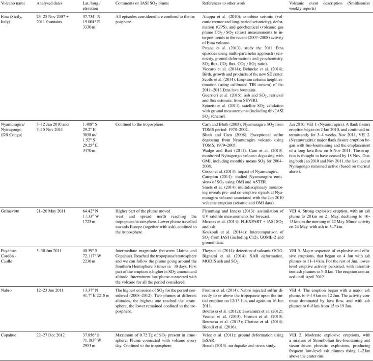
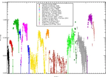
error. This is an overestimation of the error, but considering the mean squared error as total error will be an underestima-tion. This is due to the presence of systematic errors within the retrieval. The systematic errors are included within the error estimate but cannot be considered independent of each other. It is more likely that, if present, the systematic error will become a bias in the region and time considered. The time series of these total masses, together with the errors, are presented in Fig. 7 for the studied volcanic eruptions.
Using the IASI data set it is possible to follow the plume evolution of several volcanic eruptions. Within the eruptions considered, Nabro produced a maximum load of 1.6 Tg of SO2, followed by Kasatochi (0.9 Tg), Grímsvötn (0.75 Tg),
Copahue (0.72 Tg) and Sarychev (0.60 Tg). Using the time series created by this data set it might be possible to estimate the SO2lifetime, but this is beyond the scope of this work.
From the eruptions presented in Fig. 7, there is a wide spread of error bars, depending on the SO2 amount,
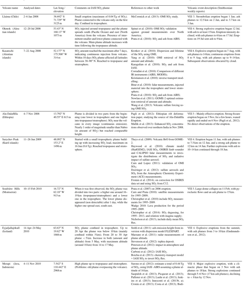
Table 1.Summary of studied eruptions, in chronological order, together with other relevant literature, volcanic explosivity index (VEI) and
a short descriptions of the events from the Smithsonian Institution Global Volcanism Programme website (http://www.volcano.si.edu).
Volcano name Analysed dates Lat./long./
elevation Comments on IASI SO2plume References to other work Volcanic event description (Smithsonianweekly reports) Llaima (Chile) 2–6 Jan 2008 38.692◦S
71.729◦W 3125 m
Small eruption (maximum of 0.04 Tg of SO2). Plume connected to the volcano only on the first day. Confined in troposphere.
McCormick et al. (2013): OMI SO2study. VEI 3. Strombolian eruption began 1 Jan; ash plumes to 12.5 km on 2 Jan, and to 3.7 km on 3 Jan.
Okmok
(Aleu-tian islands) 12–20 Jul 2008 53.43 ◦
N 168.13◦W 1073 m
SO2injected around tropopause and the plume spreads south (Pacific Ocean) and east (North America) from the volcano. Presence of inter-mittent smaller and lower plume connected with the volcano. Main plume altitude increases with time following the tropopause altitude.
Spinei et al. (2010): OMI SO2validation against ground measurements over North America;
Prata et al. (2010): SO2and ash from AIRS.
VEI 4. Strong explosive eruption began 12 Jul, with ash to at least 15 km. Eruption intensity de-clined, with ash plumes to 6 km on 17 Jul. Erup-tions on 19 Jul sent ash to 9 km.
Kasatochi (Aleutian islands)
7–22 Aug 2008 52.177◦ N 175.508◦W 314 m
SO2amount reached the maximum after 7 days, indicating continuous injection from volcano. Within 10 days SO2plume affected all latitudes between 30–90◦N. Reached to tropopause and stratosphere.
Krotkov et al. (2010): Dispersion and lifetime of the SO2using OMI;
Yang et al. (2010): OMI retrieval of SO2 amount and altitude;
Karagulian et al. (2010): SO2and ash from IASI;
Corradini et al. (2010): Comparison of different IR instruments (AIRS, MODIS); Kristiansen et al. (2010): inverse transport mod-elling;
Bitar et al. (2010): lidar measurements, injected material into the troposphere and lower strato-sphere;
Prata et al. (2010): SO2and ash from AIRS; Nowlan et al. (2011): GOME-2 optimal estima-tion retrieval of amount and altitude; Wang et al. (2013): Volcanic sulfate forcing us-ing OMI SO2.
VEI 4. Explosive eruption began on 7 Aug, with ash plumes to 14 km; continuous eruptions from 8 to 9 Aug, with ash plumes up to 9–14 km. Subsequent observations obscured by cloud.
Alu-Dalaffilla
(Ethiopia) 4–7 Nov 2008 13.792 ◦N
40.55◦E 613 m Plume is divided in two parts from the begin-ning (one lower in troposphere and one higher into tropopause/stratosphere). SO2near the vol-cano in every image (continuous emission). Nearly 1 order of magnitude smaller than Nabro (in amount of SO2) but reached comparable height.
Pagli et al. (2012): Ethiopian rift deforma-tion paper, studying the source of Alu-Dalafilla Eruption.
Mallik et al. (2013): Enhanced SO2 concentra-tions observed over northern India in Nov 2008.
VEI 3 – Mainly effusive eruption. Strong fissure eruption began on 3 Nov, for a few hours, waned rapidly and ended on 6 Nov (Pagli et al., 2012). No direct observations of the eruption.
Sarychev Peak (Kuril islands)
11–26 Jun 2009 48.092◦N 153.2◦E 1496 m
Started with a small tropospheric plume build-ing up with increasbuild-ing SO2load, maximum on 16 Jun (0.6 Tg). Reached tropopause and strato-sphere.
Theys et al. (2009): Volcanic BrO from GOME-2.
Haywood et al. (2010): climate model (HadGEM2), IASI SO2, OSIRIS limb sounder and CALIPSO lidar measurements to inves-tigate the distributions of SO2and radiative impact of sulfate aerosol;
Carn and Lopez (2011): validation of OMI SO2;
Doeringer et al. (2012): sulfate aerosols and SO2from the Atmospheric Chemistry Experi-ment (ACE) measureExperi-ments;
Fromm et al. (2014); on correction for OSIRIS data set and using SO2from C12.
VEI 4. Eruption began 11 Jun, with ash plumes to 7.5 km on 12 Jun, and a strong ash plume to 12 km on 14 Jun. Further explosions with ash to 10–14 km continued through 18 Jun.
Soufrière Hills
(Montserrat) 10–15 Feb 2010 16.72 ◦
N 62.18◦W 915 m
When it was first observed, the SO2plume was divided into two parts: a higher one around 16– 19 km (tropopause/stratosphere) and a lower one in the troposphere. The lower plume dis-appeared (non detectable) after 1 day, while the higher one spread east, south east.
Prata et al. (2007) on 2006 eruption. Carn and Prata (2010): satellite measurements for 1995–2009;
Christopher et al. (2010) include SO2 measure-ments for 1995–2009.
Wadge 2010: Lava production for the period 1995–2009.
Christopher et al. (2014): SO2degassing, for 1995– 2013, and relation with magma supply; Nicholson et al. (2013), include daily mean SO2 flux.
VEI 3. Large dome collapse on 11 Feb, with py-roclastic flows and an ash plume to 15 km.
Eyjafjallajökull (Iceland)
14 Apr–24 May 2010
63.63◦N 19.62◦
W 1666 m
SO2plume confined in troposphere. Up to 20 Apr the plume was below 10 km (mainly confined within 5 km); From 20 to 30 Apr plume<5 km. Increase in both (amount and altitude) from 5 May, with maximum altitude (around 10 km) from 14 to 17 May.
Stohl et al. (2011): ash emission height from in-version with dispersion model FLEXPART. Marzano et al. (2011): radar measurements of plume altitude.
Stevenson et al. (2012): tephra deposit. Petersen et al. (2012): impact in atmosphere and plume altitude.
Carboni et al. (2012): IASI SO2.
Boichu et al. (2013): chemistry-transport model + IASI SO2to invert SO2flux.
VEI 4. Explosive eruptions from the summit, with ash plumes from 3 to 10 km (Gudmunds-son et al., 2012).
Merapi (Java, Indonesia)
4–11 Nov 2010 7.542◦S 110.442◦ E 2968 m
High plume up to tropopause and stratosphere. (Problems: old plume overpassing the volcano).
Surono et al. (2012): estimate a total of 0.44 Tg of SO2, using IASI -AIRS assuming a plume al-titude of 16 km.
Saepuloh et al. (2013); Picquout et al. (2013); Pallister et al. (2013); Luehr et al. (2013); Jenk-ins et al. (2013); Innocenti et al. (2013b, a); Cronin et al. (2013); Costa et al. (2013); Budi-Santoso et al. (2013)
4354 E. Carboni et al.: SO2vertical distribution of volcanic plumes
Table 1.Continued.
Volcano name Analysed dates Lat./long./ elevation
Comments on IASI SO2plume References to other work Volcanic event description (Smithsonian weekly reports)
Etna (Sicily, Italy)
23–25 Nov 2007 + 2011 fountains
37.734◦N 15.004◦E 3330 m
All episodes considered are confined to the tro-posphere.
Aiuppa et al. (2010); combine seismic (vol-canic tremor and long-period seismicity), defor-mation (GPS), and geochemical (volcanic gas plume CO2/SO2ratios) measurements to in-terpret trends in the recent (2007–2008) activity of Etna volcano.
Patane et al. (2013); study the 2011 Etna episodes using multi-parameter approach (seis-micity, ground deformations and geochemistry, SO2flux, CO2flux, CO2/SO2ratio). Viccaro et al. (2014); Behncke et al. (2014); Birth, growth and products of the new SE crater. Scollo et al. (2014); Eruption column height es-timation (using calibrated TIR camera) of the 2011–2013 Etna lava fountains.
Guerrieri et al. (2015): ash and SO2, retrieval and flux estimate, from SEVIRI.
Spinetti et al. (2014), satellite SO2validation with ground measurements (including this IASI SO2scheme).
Nyamuragira/ Nyiragongo (DR Congo)
3–12 Jan 2010 and 7–15 Nov 2011
1.408◦S 29.2◦E 3058 m/ 1.52◦S 29.25◦E 3470 m
Confined to the troposphere. Carn and Bluth (2003); Nyamuragira SO2from TOMS period: 1978–2002.
Bluth and Carn (2008); Exceptional sulfur degassing from Nyamuragira volcano using TOMS, 1979–2005.
Wadge and Burt (2011). Carn et al. (2013): monitored Nyiragongo volcano degassing with OMI, including monthly means SO2for 2004– 2008.
Cuoco et al. (2013): impact of Nyamuragira. Campion (2014): studied Nyamuragira emis-sions of SO2using OMI and ASTER. Smets et al. (2014): multidisciplinary monitor-ing reveals pre- and co-eruptive signals at Nya-muragira volcano associated with the Jan 2010 volcanic eruption (seismic and OMI data).
Jan 2010, VEI 1. (Nyamuragira). A flank fissure eruption began on 2 Jan 2010, and continued in-termittently for 3–4 weeks. Nov 2011, VEI 2. (Nyamuragira): major flank fissure eruption be-gan with fire-fountaining and the emplacement of a long lava flow on 6 Nov 2011. The erup-tion is thought to have ceased by 18 Nov. Dur-ing both Jan 2010 and Nov 2011, the lava lake at Nyiragongo remained active (based on thermal alerts).
Grímsvötn 21–26 May 2011 64.42◦N 17.33◦W 1725 m
Higher part of the plume moved
west and spread north reaching the tropopause/stratosphere. Lower plume travelled towards Europe (together with ash), confined to the troposphere.
Flemming and Inness (2013): assimilation of UV satellite measurements for forecast. Moxnes et al. (2014): FLEXPART + IASI SO2 and ash.
Koukouli et al. (2014a): Intercomparison of SO2from IASI (including C12), GOME-2 and ground data.
VEI 4. Strong explosive eruption, with an ash plume to 20 km on 21 May, declining to 10– 15 km on the morning of 22 May. Minor activity on 24 May, with ash to 5–7 km.
PuyehueCordón -Caulle
5–30 Jun 2011 40.59◦S 72.117◦W 2236 m
Intermediate magnitude (between Llaima and Copahue). Reached the tropopause/stratosphere and we can follow the plume going around the Southern Hemisphere 3 times in 30 days. First part of the eruption is higher in SO2amount and altitude. Intermittent low plume connected with the volcano for all the period considered.
Theys et al. (2014): detection of volcanic OClO. Bignami et al. (2014): SAR deformation, MODIS ash and SO2.
VEI 5. Major sequence of explosive and effu-sive eruptions, that began on 4 Jun with ash plumes to 11–14 km. For the rest of Jun, lower-level eruptive activity persisted, with intermit-tent ash plumes to 5–8 km. The eruption contin-ued until April 2012.
Nabro 12–23 Jun 2011 13.37◦N 41.7◦E 2218 m
The highest emission of SO2for the period con-sidered (2008–2012). Two plumes at different altitudes, the highest one reached the strato-sphere, the lower remained confined to the tro-posphere.
Fromm et al. (2014): Nabro injected sulfur di-rectly to or above the tropopause upon the ini-tial eruption on 12/13 Jun, and again on 16 Jun 2011.
Bourassa et al. (2012); Sawamura et al. (2012); Vernier et al. (2013); Fromm et al. (2013); Bourassa et al. (2013); Clarisse et al. (2014); Biondi et al. (2016).
VEI 4. The eruption began with a major ash plume, to 9–14 km on 12 Jun. The activity con-tinue dominated by lava flow, and with ash plumes to 6–8 km from 15 to 19 Jun.
Copahue 22–27 Dec 2012 37.856◦S 71.183◦W 2953 m
Maximum of 0.72 Tg of SO2present in atmo-sphere. Plume connected with volcano every day. Confined to the troposphere.
Velez et al. (2011): ground deformation using InSAR;
Bonali (2013): earthquake and stress study.
VEI 2. Moderate explosive eruptions, with a mixture of Strombolian fire-fountaining and steam-driven phreatic explosions, producing frequent low-level ash plumes rising 1–2 km above the crater rim.
This is the main cause of the general tendency of increasing error bars with time.
It is also possible to estimate the SO2 mass present
be-tween two altitude levels. Doing this every 0.5 km bebe-tween 0 and 20 km gives a vertical distribution of SO2every∼12 h.
These results are shown, in chronological order, in Figs. 8– 11. Note that the colour-bars for different volcanic eruptions have different values, going from smaller values for Etna and Llaima eruptions to a maximum for Nabro. From these fig-ures, it is possible to observe the temporal evolution of the SO2plume as a function of altitude. These plots have to be
interpreted carefully and studied together with the maps of the amount and altitude (values and errors) because here the retrieved errors in altitude are not accounted for, and for low amounts of SO2, error in altitude can be significant. Within
the IASI spectra there is enough information to retrieve al-titude from small/medium eruptions such as Etna and Nya-muragira/Nyiragongo.
Index 0.001
0.010 0.100 1.000 10.000
SO
2
[Tg]
Llaima 2-6 Jan 2008 Okmok 12-20 July 2008 Kasatochi 7-22 Aug.2008 Dalafilla 4-7 Nov. 2008 Sarychev 11-26 June 2009 Monserrat 10-18 Feb.2010 Eyja 14 Apr.- 24 May 2010 Merapi 4-11 Nov. 2010 Etna 23-25 Nov 2007 + 2011 Congo 3-12 Jan.2010, 7-16 Nov.2011 Grim 21-26 May 2011 Puyehue 5-30 June 2011 Nabro 12-23 June 2011 Copahue 22-27 Dec. 2012
Figure 7. SO2mass present in the atmosphere as retrieved from
IASI data. The values are the measured amount every half day and vary with volcanic emission, gas removal and satellite sampling.
Points are separated by∼12 h. Data are presented in temporal
or-der along the ordinate (x axis) but eruptions are plotted
consecu-tively one after the other without a gap between them. The total
SO2amount reported here is computed using the geographic area
associated with the eruption. For eruptions which overlap in time (e.g Grimsvötn, Puyehue, and Nabro in May and June 2011) the
SO2loads within each respective area are considered and plotted
separately.
layer with a lapse rate below 2 K km−1 and lapse rate of
2 K km−1 in all layers within 2 km above this. (The
hydro-static equation is also used to convert the retrieved SO2
pres-sure into height, so any error in the prespres-sure/height conver-sion will be common to both plume and tropopause heights.) The three tropopause lines, shown in Figs. 8–11, are the mean, and the mean plus or minus the standard deviations, within the IASI plume pixels in the 12 h maps. The reported values of the tropopause are computed using the location of the volcanic pixels only. Eyjafjallajökull and Puyehue erup-tions cover the latitude range between 30 and 80◦N and
between−20 and−60◦S, respectively, thereby spanning a
large range in tropopause heights. Day-to-day variations are sometimes large due to small amounts of SO2 being
de-tected or not from 1 day to the next (coupled to the wide range of latitudes spanned by the plumes). Within the plume, the tropopause heights can differ by many kilometres espe-cially for plumes that cover a wide latitude range. As an ex-ample, the Kasatochi plume has been analysed between 30 and 90◦N. Over this range of latitudes the tropopause height
varies between 8 and 18 km. Given this caveat the lines of tropopause mean and standard deviation heights are indica-tive; e.g. a plume that is below the three lines is likely, but not necessary, confined to the troposphere, a plume that is above the three lines is likely confined in the stratosphere, and SO2
that is between the lines could be in either the troposphere or stratosphere.
In the following Sects. 5.1–5.5, we describe the eruptions shown in Figs. 8–11 grouped by geographic area. A summary of these comments together with other relevant literature and volcanic explosivity index (VEI) estimates from the Smith-sonian is given in Table 1.
Three principal factors affect plume height: (i) the ener-getics of the eruption, (ii) the dynamic effect, (iii) retrieval artefacts in the case of multilayer plumes. Here we attempt to discriminate between these factors as follows.
a. The energetics of the eruption – A crude parameter for eruption intensity and plume height is the “volcanic ex-plosivity index” or VEI. The VEI is a semi-quantitative index of eruption size, which for contemporary erup-tions can be used as a ‘threshold’ to determine the like-lihood of stratospheric injection (Newhall and Self , 1982). Eruptions of VEI 4 and larger are expected to have strong plumes and be associated with significant stratospheric injections. Eruptions of VEI 3 are interme-diate in size, with eruptive ash plumes that rise 5–15 km above the vent. Based on analysis of eruption statistics, 25–30 % of VEI 3 eruptions may reach the stratosphere (Pyle et al., 1996). Eruptions of VEI 2 and smaller are not expected to reach the stratosphere. We report these, when available, in Table 1.
b. The atmospheric effect – In the following sections we group the eruptions by geographic area in order to consider together eruptions that may have similar conditions of water vapour. Moreover we consider the tropopause altitude together with the plume altitude. c. Retrieval artefact in the case of multilayer plumes – We
do not have a way to identify this in a fresh plume but we indicate (with a black triangle) when the old plume overpasses near the volcano again (with the possibility of presence of both the old overpassing plume and the new emitted plume, at two different altitudes). The ver-tical distribution plots in Figs. 8–11 present the studied eruptions in chronological order and indicate the pres-ence of a new plume connected with the volcano with red triangular symbols at the bottom of the column.
6.1 Southern Chile: Llaima, Puyuhue–Cordón Caulle, and Copahue
In the Southern Hemisphere we analysed three eruptions that originated from volcanic activity in Chile. The wind direction was similar for each eruption, so the SO2was transported to
the east (towards South Africa).
Llaima (period analysed: 2–6 January 2008), is presented in Fig. 8. This is the smallest eruption in terms of SO2
4356 E. Carboni et al.: SO2vertical distribution of volcanic plumes 0 0.25 0.5 0.75 1 1.25 1.5 1.75 2 2.5 3 3.5 4 4.5 10 15 20 30 DU
Llaima 2–6 Jan 2008
0.000 0.001 0.002 0.003 0.004 0.005 SO 2 [Tg]
IASI SO [Tg] – Llaima 2–6 Jan 20082
2 3 4 5 6
0 5 10 15 20
2 3 4 5 6
0 5 10 15 20
Julian day from 1 Jan 2008
Altitude / km 0 0.25 0.5 0.75 1 1.25 1.5 1.75 2 2.5 3 3.5 4 4.5 10 15 20 30 DU
Okmok 12–20 Jul 2008
0.000 0.005 0.010 0.015 SO 2 [Tg]
IASI SO [Tg] – Okmok 12–20 Jul 20082
194 196 198 200 202 0
5 10 15 20
194 196 198 200 202 0
5 10 15 20
Julian day from 1 Jan 2008
Altitude / km 0 0.25 0.5 0.75 1 1.25 1.5 1.75 2 2.5 3 3.5 4 4.5 10 15 20 30 DU
Kasatochi 7–22 Aug 2008
0.00 0.02 0.04 0.06 0.08 0.10 SO 2 [Tg]
IASI SO [Tg] – Kasatochi 7–22 Aug 2008 2
220 225 230 235 0
5 10 15 20
220 225 230 235 0
5 10 15 20
Julian day from 1 Jan 2008
Altitude / km 0 0.25 0.5 0.75 1 1.25 1.5 1.75 2 2.5 3 3.5 4 4.5 10 15 20 30 DU
Dalaffilla 4–7 Nov 2008
0.000 0.005 0.010 0.015 0.020 SO 2 [Tg]
IASI SO [Tg] – Dalaffilla 4–7 Nov 20082
309 310 311 312 0
5 10 15 20
309 310 311 312 0
5 10 15 20
Julian day from 1 Jan 2008
Altitude /
km
Figure 8.The left column shows maps of the maximum SO2amount retrieved within the considered area (black rectangle). The right column
shows the SO2vertical distribution for the considered volcanic eruption. In each plot theyaxes are the vertical levels in km. The colour
represents the total mass of SO2in Tg, dark-red represents values higher than the colour-bar. Every column of the plots come from an IASI
0 0.25 0.5 0.75 1 1.25 1.5 1.75 2 2.5 3 3.5 4 4.5 10 15 20 30 DU
Sarychev 11–26 Jun 2009
0.00 0.02 0.04 0.06 0.08 SO 2 [Tg]
IASI SO [Tg] – Sarychev 11–26 Jun 20092
165 170 175 0
5 10 15 20
165 170 175 0
5 10 15 20
Julian day from 1 Jan 2009
Altitude / km 0 0.25 0.5 0.75 1 1.25 1.5 1.75 2 2.5 3 3.5 4 4.5 10 15 20 30 DU
Montserrat 10–15 Feb 2010
0.0000 0.0005 0.0010 0.0015 0.0020 0.0025 SO 2 [Tg]
IASI SO [Tg] – Montserrat 10–15 Feb 2010 2
42 43 44 45 46 0
5 10 15 20
42 43 44 45 46 0
5 10 15 20
Julian day from 1 Jan 2010
Altitude / km 0 0.25 0.5 0.75 1 1.25 1.5 1.75 2 2.5 3 3.5 4 4.5 10 15 20 30 DU
Eyjafjallajokull 14 Apr–24 May 2010
0.000 0.002 0.004 0.006 0.008 0.010 SO 2 [Tg]
IASI SO [Tg] – Eyjafjallajokull 14 Apr–24 May 20102
110 120 130 140 0
5 10 15 20
110 120 130 140 0
5 10 15 20
Julian day from 1 Jan 2010
Altitude / km 0 0.25 0.5 0.75 1 1.25 1.5 1.75 2 2.5 3 3.5 4 4.5 10 15 20 30 DU
Merapi 4–11 Nov 2010
0.00 0.01 0.02 0.03 SO 2 [Tg]
IASI SO [Tg] – Merapi 4–11 Nov 20102
308 310 312 314 0
5 10 15 20
308 310 312 314 0
5 10 15 20
Julian day from 1 Jan 2010
Altitude /
km
4358 E. Carboni et al.: SO2vertical distribution of volcanic plumes 0 0.25 0.5 0.75 1 1.25 1.5 1.75 2 2.5 3 3.5 4 4.5 10 15 20 30 DU
Etna 23–25 No v 2007 + 2011
0.0000 0.0005 0.0010 0.0015 0.0020 SO 2 [Tg]
IASI SO [Tg] – Etna 23–25 Nov 2007 + 20112
0 5 10 15 20 0 5 10 15 20
E.C. 22:51 28/01/16.
Altitude /
km
a b c d e f g h i j k l m n o p q r
0 0.25 0.5 0.75 1 1.25 1.5 1.75 2 2.5 3 3.5 4 4.5 10 15 20 30 DU
Nyiamuragira/Nyiragongo 2010–2011 IASI SO [Tg] – Nyiamuragira/Nyiragongo 2010–20112
4 6 8 10 12 0
5 10 15 20
4 6 8 10 12 0
5 10 15 20
Julian day from 1 Jan 2010
Altitude /
km
676 678 680 682 684 0
5 10 15 20
676 678 680 682 684 0
5 10 15 20
Julian day from 1 Jan 2010 0.00 0.01 0.02 0.03 0.04 0 0.25 0.5 0.75 1 1.25 1.5 1.75 2 2.5 3 3.5 4 4.5 10 15 20 30 DU
Grimsvotn 21–26 May 2011
0.00 0.02 0.04 0.06 0.08 SO 2 [Tg]
IASI SO [Tg] – Grimsvotn 21–26 May 2011 2
142 143 144 145 146 0
5 10 15 20
142 143 144 145 146 0
5 10 15 20
Julian day from 1 Jan 2011
Altitude / km 0 0.25 0.5 0.75 1 1.25 1.5 1.75 2 2.5 3 3.5 4 4.5 10 15 20 30 DU
Puyehue 5–30 Jun 2011
0.000 0.002 0.004 0.006 0.008 0.010 0.012 SO 2 [Tg]
IASI SO [Tg] – Puyehue 5–30 Jun 20112
160 165 170 175 180 0
5 10 15 20
160 165 170 175 180 0
5 10 15 20
Julian day from 1 Jan 2011
Altitude /
km
Figure 10.As for Fig. 8. The Etna plots show different eruptive episodes corresponding toxaxes labels:(a)23–25 November 2007 eruption;
and the 2011 lava fountains:(b)11–13 January,(c)17–19 February,(d)10–12 April,(e)11–13 May,(f)8–10 July,(g)18–20 July,(h)24–
26 July, (i)29 July–1 August,(j) 4–7 August,(k) 11–13 August,(l) 19–21 August,(m) 28–30 August,(n) 7–10 September,(o)18–
0 0.25 0.5 0.75 1 1.25 1.5 1.75 2 2.5 3 3.5 4 4.5 10 15 20 30 DU
Nabro 12–2 3 Jun 2011
0.00 0.02 0.04 0.06 0.08 0.10 SO 2 [Tg]
IASI SO [Tg] – Nabro 12–23 Jun 20112
164 166 168 170 172 174 0
5 10 15 20
164 166 168 170 172 174 0
5 10 15 20
Julian day from 1 Jan 2011
Altitude / km 0 0.25 0.5 0.75 1 1.25 1.5 1.75 2 2.5 3 3.5 4 4.5 10 15 20 30 DU
Copahue 22–27 Dec 2012
0.00 0.05 0.10 0.15 0.20 SO 2 [Tg]
IASI SO [Tg] – Copahue 22–27 Dec 20122
357 358 359 360 361 362 0
5 10 15 20
357 358 359 360 361 362 0
5 10 15 20
Julian day from 1 Jan 2012
Altitude /
km
Figure 11.As for Fig. 8.
VEI 3 VEI 4 VEI 5 H e ig h t [k m ] Ll a im a O k m o k K a sa to ch i D a la fi ll a S a ry ch e v M o n ts e rr a t E y ja M e ra p i G ri m P u y e h u e N a b ro
Figure 12.Eruption SO2-plume altitudes from this study. The black
lines show the range of altitudes retrieved, the boxes depict the
al-titude range into which the 50 % of the SO2mass falls, the
hori-zontal lines within each box are the altitudes of the maximum of
SO2mass. Different colours represent eruptions of different VEI
(Source: Global Volcanism Program, 2013).
Copahue (22–27 December 2012), in Fig. 11, released a higher amount of SO2(up to 0.72 Tg of atmospheric load)
and there was a continuous plume from the volcano, indicat-ing that the volcano emitted SO2for at least 7 days. Both of
these eruptions remained confined to the troposphere.
The Puyehue–Cordón-Caulle eruption of 5–30 June 2011 was the most significant eruption in southern Chile since 1991. The eruption commenced with the formation of a very significant eruption plume, that was tracked around the globe, and sustained lower-level activity that continued in-termittently during the observation period. This eruption was between Llaima and Copahue in terms of SO2amount
(max-imum load of 0.13 Tg), but higher than both in terms of VEI (with a value of 5), and with a much higher altitude (Fig. 11). The first part of the eruption produced a higher plume in terms of amount and altitude, and a lower plume connected with the volcano was present intermittently for all of the pe-riod observed. The maximum amount of SO2loading found
was 0.13±0.06 Tg on 8 and 9 June. Theys et al. (2013)
present the SO2amount from the Clarisse et al. (2012) IASI
scheme, assuming an altitude of 13 km, and reported values around 0.14 Tg (and higher) for the periods 6–9 June, with a maximum on 7 June. The fresh part of the plume (over South America and the western Atlantic Ocean) is found to be significantly lower using C12 (between 2 and 5 km of al-titude) than the altitude of 13 km assumed by Theys et al. (2013), and the SO2amount for a plume at 5 km will be
un-derestimated using the assumption of higher altitude. Due to the opposite effect, the presence of SO2higher than 13 km
in the first 2 days may explain the discrepancy in the SO2
load (Fig. 2 from Theys et al., 2013 reports higher SO2than
4360 E. Carboni et al.: SO2vertical distribution of volcanic plumes
retrieval as assumptions regarding plume altitude may lead to significant differences in SO2total mass estimates.
6.2 Northern Pacific Ocean: Okmok, Kasatochi, and Sarychev
Okmok, Kasatochi and Sarychev eruptions (Figs. 8 and 9) all affected the boreal atmosphere and injected SO2to altitudes
around the tropopause (and higher).
Okmok (12–20 July 2008) injected SO2around 12 km and
the plume spread south and east from the volcano, over the Pacific Ocean. The main plume reached the US and Canada, and there was an intermittent presence of a small and low plume connected with the volcano.
Kasatochi (7–22 August 2008) injected the majority amount of SO2within the first 3 days and the plume spread
around the Northern Hemisphere, going east, north and west from the volcano. The SO2 amount reached a maximum
7 days after the start of the eruption, indicating continu-ous injection from the volcano. Within the first 10 days of the eruption it affected the latitude bands 30 to 90◦N. The
SO2 amounts for the first days of the eruption are in the
ranges reported from Corradini et al. (2010) for AIRS and MODIS estimates. (Corradini et al., 2010 report AIRS and MODIS 7.3 µm SO2mass loadings between 0.3 and 1.2 Tg,
while the MODIS ash corrected 8.7 µm SO2masses vary
be-tween 0.4 and 2.7 Tg). The altitude retrieved using C12 for Kasatochi is consistent with 12.5±4 km reported by
Karag-ulian et al. (2010), but the total SO2 load is around 30 %
lower. Karagulian et al. (2010) use an IASI retrieval from
ν3 band (1362 cm−1) and ν1+ν3 band (2500 cm−1). The
altitudes from C12 are also comparable with the range re-ported in CALIPSO and OMI data from Wang et al. (2013) (Wang et al., 2013 used the OMI retrieval of altitude and amount and GEOS-Chem models to estimate that the forc-ing by Kasatochi volcanic sulfate aerosol became negligible 6 months after the eruption).
Sarychev is located at a similar latitude as Kasatochi, but in the Kurile islands south of Kamchatka. The IASI SO2
scheme, C12, (similar to that previously reported by the Uni-versité Libre de Bruxelles, IASI-ULB, near real-time SO2
alert system, http://cpm-ws4.ulb.ac.be/Alerts/index.php, Rix et al., 2009; Haywood et al., 2010), retrieves a small tropo-spheric plume in the two images from 11 June 2009, followed by a higher plume on 12 June. The SO2loading increased in
the following days (with a big injection the 15 June 2009) reaching a maximum on 16 June (0.6 Tg). Then the SO2load
remained approximately constant for 16–18 June, before de-creasing after that. The plume went in two directions, one branch spreading across the Pacific Ocean to North America and crossing Canada, reaching the Atlantic Ocean on 22 June and the Spanish coast of Europe on 24 June; the second branch went north, crossing Siberia up to the Siberian Sea and turning east to Greenland.
6.3 Africa: Dalafilla, Nabro
Two volcanic eruptions from the Ethiopian Rift, Dalafilla in November 2008 and Nabro in June 2011, had a lower plume around 4–6 km and a higher part of the plume around the tropopause, but they were nearly 1 order of magnitude dif-ferent in terms of SO2amount. Dalafilla produced a
maxi-mum SO2atmospheric loading of 0.2 Tg while Nabro
pro-duced 1.6 Tg. This could be the result of volcanic effects (for example Dalafilla was a very short-lived and vigorous fire-fountaining eruption from an extended fissure that produced, in some parts low mass eruption rates and in other parts much higher eruption rates. Another possible explanation of how a medium/small eruption such as Dalafilla (VEI 3) reached the tropopause altitude is illustrated in Tupper et al. (2009) and implicated the effect of a moist atmosphere. Tupper et al. (2009) showed that volcanic emissions with different erup-tion rates in moist atmosphere both reached the tropopause; in dry atmosphere they reach different altitudes.
The first IASI observation showing the Dalafilla eruption was at 05:00 UTC on 4 November 2008. The plume is di-vided into a lower and a higher part. These spread north and east from Ethiopia, covering the Arabic Peninsula, and ar-rived over north India and the Himalayas on the 5 Novem-ber. They then spread over China, and a diluted plume ar-rived over south Japan on 6 November. IASI detected SO2
near the volcano in every image in this period. According to Meteosat-9 false colour RGB images, the eruption started between 12:45 UTC and 13:00 UTC on 3 November 2008, with high-level SO2 plumes and an ash plume (mixed with
ice). The low-level SO2plume, started 3 hours later2.
The IASI images of SO2 amount and altitude are
consis-tent with the measurements over northern India reported by Mallik et al. (2013). In particular, Mallik et al. (2013) report the following: (i) high concentration of column SO2 from
ground measurements where the time of exceptionally high SO2amount is consistent with the IASI plume arriving over
the Indian location; (ii) CALIPSO observations of a scat-tering feature around 4–5 km altitude on 6 November that is consistent with the lower part of the plume reported here by IASI; (iii) OMI maps, obtained assuming a fixed altitude, with a position of the SO2plume similar to IASI. With the
use of C12 IASI scheme it is possible to discern that there is both a lower plume in the troposphere (as reported by Mallik et al., 2013) and a significant part of the plume at altitudes around the tropopause.
Nabro produced the largest amount of SO2 in any
vol-canic plume observed by IASI with a maximum of up to 1.6±0.3 Tg of SO2.
Numerous previous studies have documented this erup-tion, with many of them focusing on whether Nabro injected SO2 directly into the stratosphere or whether the injection
2http://www.eumetsat.int/website/home/Images/ImageLibrary/
was associated with monsoon circulation (Bourassa et al., 2012, 2013; Sawamura et al., 2012; Vernier et al., 2013; Fromm et al., 2013, 2014; Clarisse et al., 2014; Biondi et al., 2016).
A more detailed study of the Nabro eruption, also us-ing the C12 IASI retrieval scheme, is reported in Fromm et al. (2014), and concluded that “Nabro injected sulphur di-rectly to or above the tropopause upon the initial eruption on 12/13 June, and again on 16 June 2011”. Here we include
the Nabro summary of the C12 IASI data set. The Nabro plume is retrieved on 13 June, with a plume over north-east Africa between 14 and 18 km height. On the 14 the plume ar-rived over the Middle East and over central Asia on 15 June. The eruption formed two plumes at different altitudes, the higher one that reached the stratosphere and a lower one that remained confined to the troposphere with less than 10 km altitude. The higher plume is further separated into two seg-ments, a “north” one (15 km and above) and a “south” one, a bit lower. Over all these days the plume was still attached to the volcano, indicating continuous injection. On 17 June there is a lower altitude plume and a new high altitude part going over north-east Africa.
In Fromm et al. (2014) two comparisons have demon-strated the consistency of IASI altitude with other measure-ments: (i) morning and afternoon IASI data of the 14 June are compared with the lidar ground data at Sede Boker (Israel) and an SO2profile from MLS (Fromm et al., 2014; Fig. 8);
(ii) the night time IASI measurements of 17 June are com-pared with the CALIOP and MLS measurements (Fromm et al., 2014; Fig. 9).
6.4 Iceland: Eyjafjallajökull and Grímsvötn
Eruptions of Eyjafjallajökull in April and May 2010 and Grímsvötn in May 2011 have been examined. A deeper anal-ysis of the IASI SO2plume from the Eyjafjallajökull
erup-tion is presented in Carboni et al. (2012) and here we only report the time series of vertical distribution.
The first IASI observation of the Eyjafjallajökull plume is in the evening of 14 April 2010. The SO2 plume altitudes
retrieved in successive observations up to 20 April are be-low 10 km, mainly confined bebe-low 5 km. Small amounts of SO2between 16 and 20 April are between 5 and 10 km in
altitude. From 20 to 30 April, SO2 is always below 5 km.
There is a little increase of SO2amount and altitude on the
1 and 2 May, and a more pronounced increase of both SO2
amount and altitude from the 5 May. The retrieved altitude has a maximum during the 14–17 May period, where values reach around 10 km.
Grímsvötn’s plume was first observed by IASI on the morning of 22 May 2011. From the afternoon of 22 May it is possible to see an SO2rich plume going north, with a
seg-ment going north-east, and a lower plume going south/south-east. The denser part of the higher SO2plume moved west
and arrived over Greenland, and out of the analysed area
on 24 May. This segment re-entered the analysed area on 26 May in the afternoon (this is why the last column of the plot has an apparent increase in SO2). The lower
alti-tude plume, moving in south/south-east direction, is reported to be more ash rich (Moxnes et al., 2014) and travelled to-wards Europe, arriving over the northern UK on 24 May in the morning, and over Scandinavia in the afternoon. These observations of the Grímsvötn eruption do not completely represent the total atmospheric SO2due to the fact that a part
of the plume is missing.
6.5 Minor frequent events: Etna and Congo
The activity of Etna and Nyamuragira/Nyiragongo during the period was limited to smaller eruptions and lava fountains. Here we do not report an exhaustive list of these episodes, but a few examples to show how these emissions can be observed by IASI. The Smithsonian Institution reported that Nyamura-gira erupted on 2 January 2010 and 6 November 2011. From IASI data it is not possible to distinguish between Nyamura-gira and Nyriagongo emissions, but SO2plumes are observed
from 3 to 12 January 2010 and from 7 to 15 November 2011. The SO2 plumes spread over the equatorial area of Africa
from Congo up to Sudan and Chad, with decreasing SO2
loading away from the volcano. The main plumes were con-fined to the troposphere and disappeared after a few days.
The Etna events considered are the 23–25 November 2007 eruption and the 2011 lava fountains: 11–13 January, 17– 19 February, 9–12 April, 11–13 May, 8–10 July, 18–20 July, 24–26 July, 29 July, 1 August, 4–7 August, 11–13 Au-gust, 19–21 AuAu-gust, 28–30 AuAu-gust, 7–10 September, 18– 20 September, 27–30 September, 12–17 November. Analy-sis was performed for the lava fountain period plus one day either side. The Etna eruption in 2007 produced the high-est SO2 atmospheric loading for the period analysed (more
than 0.1 Tg). The lava fountains are associated with smaller amounts of SO2and with large error. Etna emissions are
ap-proximately 10 times smaller than those from the Congo. In particular, the SO2 for 2011 Etna fountains have been
validated within the SAMSH-SACS2 project and the SO2
amount measured by IASI are consistent with ground obser-vation (Spinetti et al., 2014).
We now examine, for these eruptions, whether the VEI and SO2-plume height are correlated or not. The definition
of eruption altitude is not straightforward due to the change in plume altitude (in both space and time). The values of VEI in this study were taken from the (Global Volcanism Pro-gram, 2013) updated through 2015. VEI estimates may be subject to revision, but for contemporary eruptions, they typ-ically refer to the “peak” phase of the eruption; they are not good descriptors for long-lived eruptions (e.g. Montserrat), or eruptions of variable intensity. Figure 12 shows different plume altitudes, and altitude ranges, for the eruptions with VEI 3, 4 and 5. The altitudes where the 50 % SO2mass is