Abstract
This work presents a metamodel strategy to approximate the buckling load response of laminated composite plates. In order to obtain representative data for training the metamodel, some lami-nates with different stacking sequences are generated using the Latin hypercube sampling plan. These stacking sequences are converted into lamination parameters so that the number of in-puts of the metamodel becomes constant. The buckling load for each laminate of the training set are computed using finite ele-ments. In this way the inputs-outputs metamodel training pairs are the lamination parameters and the corresponding bucking load. Neural network and support vector regression metamodels are employed to approximate the buckling load. The performances of the metamodels are compared in a test case and the results are shown and discussed.
Keywords
Composite laminate, lamination parameters, buckling, support vector regression, neural network.
Laminated Composites Buckling Analysis
Using Lamination Parameters, Neural Networks
and Support Vector Regression
1 INTRODUCTION
Laminated composite materials are made from layers which usually consist of two distinct phases: matrix and fibers. The fibers (e.g. carbon, glass, aramid) are embedded in a polymeric matrix. In a single layer (or ply) the fibers are oriented in a certain direction and when many layers are stacked together, making a laminate, each one can be tailored with a different orientation with each other. Specific properties and mechanical behavior of laminated composites can be found in Jones (1999), Staab (1999) or Mendonça (2005). The definition of the best orientation angle for each ply usually demands a great amount of computational time for complex structures, even when optimization algorithms are used. One option, in order to reduce the computational cost in the optimization pro-cess, is to use metamodels. A metamodel (also called surrogate model) is a mathematical model
Rubem M. Koide a Ana Paula C. S. Ferreira a Marco A. Luersen a
a Laboratório de Mecânica Estrutural
(LaMEs), Universidade Tecnológica Fe-deral do Paraná (UTFPR), Curitiba, PR, Brazil.
[email protected] [email protected] [email protected]
http://dx.doi.org/10.1590/1679-78251237
Latin A m erican Journal of Solids and Structures 12 (2015) 271-294
trained to represent or simulate a phenomenon. The training process is performed based on input-desired output training pairs, that is, the metamodel receives inputs and input-desired outputs and its parameters are adjusted in order to reduce the error between the metamodel output and the desired output. The selection of the metamodel training inputs can be performed randomly or planned aim-ing to explore a representative set of values of the design variables. The latter is called designs of experiments (DOE).
This works aims to analyze the laminated composites buckling using lamination parameters, neural networks and support vector regression. The knowledge of critical buckling load is important in the design of thin structures such as laminated composites. The first step of our approach is to apply the Latin hypercube DOE technique (Meyers and Montgomery, 2002) to obtain the stacking sequence samples for the training input laminates. The second step is to convert the laminate stack-ing sequences (i.e., the set of ply angle orientations) into lamination parameters. This is done in order to have a constant number of inputs for the metamodel. Then, the buckling load for each laminate configuration is computed with the commercial finite element code Abaqus. This is the third step and provides the outputs for training the metamodel. Once the training pairs are ob-tained, the final step is to train the metamodels and evaluate their performances in a test case. Hence, the objective of this study is to compare the ability of neural network and support vector regression metamodels in estimating buckling load. The buckling load response computed by finite element and its approximation by neural network and by support vector regression are presented in order to verify which of these metamodels is the most suitable for the present application. Statisti-cal analysis using the correlation factor is adopted to compare the performance of the different metamodels.
2 BUCKLING OF LAMINATED COMPOSITES
As the structures of laminated composites are usually thin and subject to compressive loads, they are susceptible to buckling. The analyses of buckling behavior are, in general, conducted to maxim-ize the buckling load in order to obtain a reliable and lightweight safe structure.General buckling theory for laminated composites can be found in Jones (1999). More specifically, Leissa (1983) pre-sented classical buckling studies with mathematical and physical approaches. The subject is treated with classical bifurcation buckling analysis, plate equations and their solutions. Analytical analysis and development prediction of buckling and postbuckling is stated by Arnold and Mayers (1984). Sundaresan et al. (1996) studied the buckling of thick laminated rectangular plates adopting the
Latin A m erican Journal of Solids and Structures 12 (2015) 271-294
(2010). Kalnins et al. (2009) used the metamodel approach for optimization of postbuckling re-sponse. Artificial neural networks have been used by Bezerra et al. (2007) to approximate the shear mechanical properties of reinforced composites. Reddy et al. (2011) optimized the stacking sequence of laminated composite plates applying neural network. Their work included experimental and finite element analysis for minimizing the deflections and stresses. In the step of validation tests, they evaluated the quality of the results of the predicted outputs and the experimental measured outputs using a regression coefficient. The high correlation between the predicted values by neural network and finite element analysis validated the metamodel. Reddy et al. (2012) studied the D-optimal design sampling plan and artificial neural network in the natural frequency prediction of laminated composite plates. Todoroki et al. (2011) proposed a Kriging surrogate model in order to predict and maximize the fracture load of laminated composites using lamination parameters. Lamination pa-rameters were also adopted by Liu et al. (2010) in the optimization of blended composite wing pan-els using smeared stiffness technique and by Herencia et al. (2007) in the optimization of long aniso-tropic fiber-reinforced laminate composite panels with T-shaped stiffeners.
This work presents artificial neural network (ANN or simply NN) and support vector machine (SVM) metamodels of a laminated composite plate. The metamodels are trained with lamination parameters as inputs. The desired outputs are the composite plate buckling loads, which are com-puted by a finite element model. The goal is to investigate which metamodel performs better in this application. The methodology of design of experiments and metamodeling is applied in the numeric case to obtain the buckling response and the results are presented and discussed. A summary about the learning formulation, lamination parameters and Latin hypercube sampling technique are pre-sented.
2.1 Lamination parameters
Lamination parameters are the extension of the invariant concepts for a lamina to a laminate pro-posed by Tsai and Pagano (1968) and are described here based on Jones (1999) and Foldager et al. (1998).
The transformed stiffnessess of an orthotropic composite ply is written as
4 4 2 2 2 2
11 11 22 12 66
4 4 2 2 2 2
22 11 22 12 66
2 2 2 2 4 4 2 2
12 21 11 22 12 66
2
2 2 2 2 2 2 2 2
66 11 22 12 66
3 3 3 3 3 3
16 61 11 22 12 66
3
26 11
2 4
2 4
4
2
2 Q m Q n Q m n Q m n Q
Q n Q m Q m n Q m n Q
Q Q m n Q m n Q m n Q m n Q
Q m n Q m n Q m n Q m n Q
Q Q m nQ mn Q mn m n Q mn m n Q
Q mn Q
3
3 3
3 3
22 12 2 66
m nQ m nmn Q m nmn Q
Latin A m erican Journal of Solids and Structures 12 (2015) 271-294 where
11 1 12 21
22 2 12 21
12 12 2 12 21
66 12 1 1 1 cos sin Q E Q E Q E Q G m n (2)
Looking at (Eq. (1)), it is difficult to understand what happens to a laminate when it is rotated. Motivated by that fact, Tsai and Pagano (1968) recasted the transformed stiffnessess and obtained what is called invariants, which are written as
1 11 22 12 66
2 11 22
3 11 22 12 66
4 11 22 12 66
5 11 22 12 66
3 3 2 4 / 8
/ 2
2 4 / 8
6 4 / 8
2 4 / 8
U Q Q Q Q
U Q Q
U Q Q Q Q
U Q Q Q Q
U Q Q Q Q
(3)
The invariants can be used to rewrite the transformed stiffnesses of an orthotropic lamina
11 1 2 3
22 1 2 3
12 4 3
66 5 3
16 2 3
26 2 3
cos 2 cos 4
cos 2 cos 4
cos 4
cos 4 1
sin 2 sin 4 2
1
sin 2 sin 4 2
Q U U U
Q U U U
Q U U
Q U U
Q U U
Q U U
(4)
Looking at Eq. (4), it is possible to note that the transformed stiffnesses’ eleme“ts Q11, Q22, Q12 and Q66 computed with the invariants have as first terms in their equations the invariants U1, U4 and U5, which depend only on the material properties. The use of invariants makes easier to
under-stand how the lamina stiffness is composed. For example,Q11 is determined by U1, plus a second term of low-frequency variation with , and another term of higher frequency. Hence, U1 represents
an effective measure of lamina stiffness because it is not influenced by orientation (Jones, 1999). The laminate stiffness matrices [A], [B] and [D] in terms of a matrix of invariants [U] and the lamination parameters {A,B,D can be written in a vector form as
Latin A m erican Journal of Solids and Structures 12 (2015) 271-294
where t is the total thickness of the laminate and [U] is the matrix of invariants set and it is given by
1 2 3
1 2 3
1 4 3 4 3 2 3 2 3 0 0 0 0
0 0 0
2
0 0 0
0 0 0
2
0 0 0
2
U U U
U U U
U U
U
U U U
U U U U (6)
The lamination parameters are written as
1 1,2,3,4 1 2 2 1 1,2,3,4 2 1 3 3 1 1,2,3,4 3 1 1
( )[cos 2 sin 2 cos 4 sin 4 ]
2
( )[cos 2 sin 2 cos 4 sin 4 ]
4
( )[cos 2 sin 2 cos 4 sin 4 ]
N A
k k k k k k
K N B
k k k k k k
K N D
k k k k k k
K z z t z z t z z t
(7)The matrix [A] and the vector {A} has the following correspondence:
11
22
11 12 16
66
12 22 26
12
16 26 66
16
26
[ ]
A
A A A A
A
A A A A A
A A A A
A A (8)
and the same is done for matrices [B] and [D].
Latin A m erican Journal of Solids and Structures 12 (2015) 271-294
3 DESIGN OF EXPERIMENTS AND METAMODELING
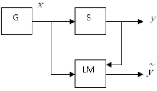
As already mentioned, the technique to plan the number and location of the sampling points in the design space is called design of experiments (DOE). A metamodel or surrogate model is generated from experimental tests or computer simulations. It uses mathematical functions to approximate highly complex objective in the design problems (Liao et al., 2008). Metamodeling approach (some-times also called response surface methodology) has been used for the development and the im-provement of designs and processes. Meyers and Montgomery (2002) defined the response surface as a collection of statistical and mathematical techniques for development, improving and optimiz-ing processes. Simpson et al. (2008) and Wang and Shan (2007) reviewed this subject, focusoptimiz-ing on sampling, model fitting, model validation, design space exploration and optimization methods. An approximate function or response is searched based on sequential exploration of the region of inter-est. The basic metamodeling technique has the following steps: sample the design space, build a metamodel and validate the metamodel (Wang and Shan, 2007). There are many experimental de-signs plans to sample the space such as central composite, box-behnken, Latin hypercube, Monte Carlo (Meyers and Montgomery, 2002). A review study and comparison of several sampling criteria are presented by Janouchova and Kucerova (2013). There are also many metamodels techniques such as Kriging, radial basis functions, artificial neural network, decision tree and support vector machine (Wang and Shan, 2007 and Vapnik, 2000). Suttorp and Igel (2006) defined support vector machine as a learning machine strategy based on a learning algorithm and on a specific kernel that computes the inner product of an input set of points in a feature space. In this work, Latin hyper-cube design is applied and also two metamodels based on learning machine, neural network and support vector regression (SVR), are used. In this case, learning is a problem of function estimation based on empirical data as explained Vapnik (2000). Vapnik proposed this approach in the 1970s. In the analysis of learning processes, inductive principle is applied with high ability and the ma-chine learning algorithm is generated by this principle. The learning mama-chine model is usually rep-resented by three components (Vapnik, 2000). First, a generator of random vector G( ) or the in-put data; second, a supervisor (S) which returns an outin-put value ; and third, a learning machine (LM) that implements a set of functions that approximates the supervis”r’s resp”“se . Figure 1 shows a schematic representation of a learning model.
Latin A m erican Journal of Solids and Structures 12 (2015) 271-294
3.1 Latin Hypercube Design
Latin hypercube (LH) design is a DOE strategy to choose the sampling points. Pan et al. (2010) stated that LH is one of the space-filli“g meth”ds i“ which all regi”“s ”f desig“ space are consid-ered equal, and the sampled points fill the entire design space uniformly. Forrester et al. (2008) explained that LH sampling generates points by stratification of sampling plan on all of its dimen-sions. Random points are generated by projections onto the variable axes in a uniform distribution. A Latin square or square matrix n x n is built filling every column and every line with permutation
”f {1, 2, … , n} as stated by Forrester et al. (2008). Following in this way, every number must be selected only once in all axes. A simple example of a Latin hypercube with n = 4 is presented in Table 1, where each line represents one sample that constructs the input sampling data with uni-form distribution.
Latin hypercube
2 3 1 4
3 2 4 1
1 4 3 2
4 1 2 3
Table 1: Latin square sampling example.
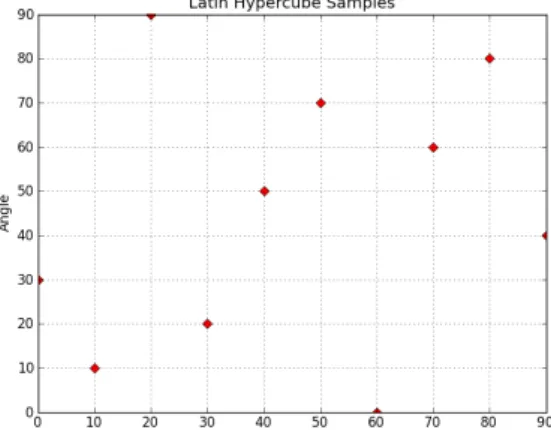
The variables are uniformly distributed in the range [0,1]. The normalization is used for multidi-mensional hypercube, where the samples of size n xm variables are randomly selected considering the mpermutati”“s ”f the seque“ce ”f i“tegers 1, 2, … ,n and assigning them to each of the m col-umns of the table (Cheng and Druzdzel, 2000). In the multidimensional Latin hypercube the design space is divided into an equal sized hypercube and a point is placed in each one (Forrester et al., 2008). As an example, a ten-point Latin hypercube sampling plan for a laminated of two layers is shown in Figure 2. The design based on two variables, the lamination angles, ranged from 0 to 90, is selected randomly with the uniform distribution. If the problem has numerous design variables, the computational demand also increases. However, using some DOE technique, for example, Latin hypercube, data sampling can be generated, which is able to better represent the design space and, as a consequence, more accurate models can be obtained with less points, and subsequently decrease the computational time.
Latin A m erican Journal of Solids and Structures 12 (2015) 271-294
In this work, the ply angle orientations are converted into lamination parameters in order to keep the number of inputs constant for the metamodels, independently of the number of layers of the laminate.
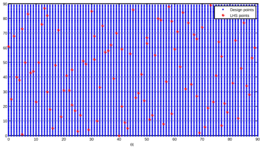
Figure 3 shows the design space of a four-layer symmetric laminate, which has only two design var-iables (1 and 2). This design space considers the plies angular orientations varying in the range [0 90] with increments of one degree (blue points). The red points are the laminates selected by the LHS. Figure 4 shows the design space of the same laminate, but considering lamination parameters. It means that the lamination parameters are computed for each laminate of Fig. 3 and showed as the blue dots in Fig. 4. The laminates selected by the LHS are also highlighted in lamination pa-rameters design space as the red dots. It is possible to see that they are uniformly distributed in both design space.
These figures also show that the angular orientation design space is completely filled and each laminate has corresponding lamination parameter. On the other hand, the lamination parameters design space ranges from -1 to 1, but there is some empty regions in the space. It means that some lamination parameters do not have a correspondent laminate. In this way, it can be concluded that for optimization purposes it is not possible to considers only the lamination parameters design space because the result can be a non existent laminate. Foldager et al. (1998) presented an approach to deal with this fact.
Figure 3: Design space considering angular orientation.
Figure 4: Design space considering lamination parameters and .
0 10 20 30 40 50 60 70 80 90
0 10 20 30 40 50 60 70 80 90
Design points LHS points
-1 -0.8 -0.6 -0.4 -0.2 0 0.2 0.4 0.6 0.8 1
0 0.1 0.2 0.3 0.4 0.5 0.6 0.7 0.8 0.9 1
Latin A m erican Journal of Solids and Structures 12 (2015) 271-294
3.2 Neural network
Neural network studies have started by the end of the 19th and the beginning of the 20th century. By this time researchers have started to think about general learning theories, vision, conditioning, etc. The mathematical model of a neuron was created in the 1940’s and the first application of neu-ral networks was about ten years later with the perceptron and the ADALINE (ADAptive Linear Neuron). The ADALINE and the perceptron are similar neural networks with a single layer. The first one uses the transfer linear function and the second one uses hard limiting function. The per-ceptron is trained with the perper-ceptron learning rule and the ADALINE with the Least Mean Squared (LMS) algorithm. They both have the same limitation that is to only solve linearly separa-ble prosepara-blems. This limitation was overcome i“ the 1980’s with the development of the backpropagation algorithm. It is a generalization of the LMS algorithm used to train multilayer networks. As the LMS, the backpropagation is an approximate steepest descent algorithm. The difference is that in the ADALINE the error is a linear explicit function of the network weights and its derivatives with respect to the weights can be easily computed. The backpropagation, by its time, is for multilayer networks with nonlinear transfer functions and the computation of the deriv-atives with respect the weights require chain rule. This means that the error must be backpropagated by the multilayer neural network in the process of updating the weights (Hagan et al., 1996).
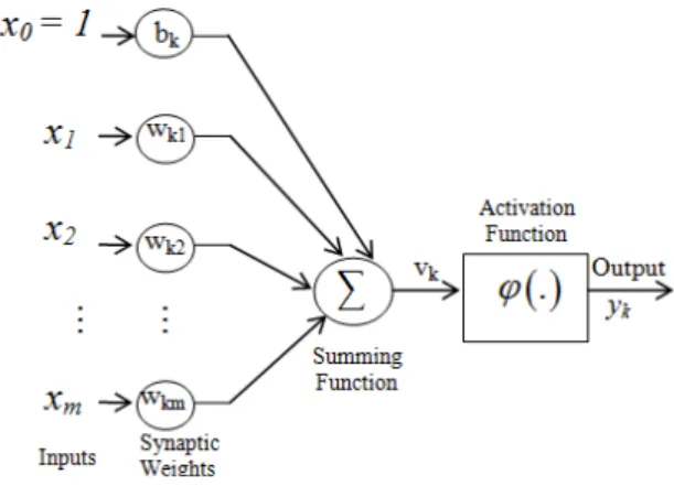
Figure 5 shows the model of a neuron used in a multilayer neural network.
Figure 5: Nonlinear model of a neuron (Haykin, 1999).
It receives some inputs (xi) that are multiplied by synaptic weights (wki). The bias (bk) are weights
with constant input equal to one. The sum of these weighted inputs (vk) has its amplitude limited
by the activation function (φ (.)). The neuron output (yk) is given by
1
m
k kj j k
j
k k
v w x b
y v
Latin A m erican Journal of Solids and Structures 12 (2015) 271-294
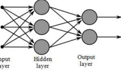
One multilayer network is represented in Figure 6. It has one input layer, one layer of hidden neu-rons and one layer of output neuneu-rons. By adding one or more hidden layers, the network is able to extract higher-order statistics, which is important when the size of the input layer is large (Haykin, 1999).
Figure 6: Multilayer neural network.
The neural network can be trained by supervised or unsupervised learning. The unsupervised learn-ing uses competitive learnlearn-ing rule and it is not the subject of this work. Supervised learnlearn-ing needs a desired output to be compared with the neural network output and return an error. The learning process is based on error correction. Error measurement is a nonlinear function of the network pa-rameters (weights and bias) and numerical analysis methods for the minimization of functions may be applied. The error minimization process is performed with the weights and bias adjustment using the backpropagation algorithm or one of its variations. It is described here based on Haykin (1999). The function to minimize is the mean squared error, which is written as
Tk k
F w e e (10)
where { } is a vector with the weights and bias of the neural network neuron k and {ek} is the
error vector at the n-th iteration.
The weights and bias are updated according to the following rules
1 1
1
T
m m m m
n n
m m m
n n
W W S y
b b S
(11)
where [W] is a matrix with the weights of the m-th neural network layer ,
is the rate of learningand
S m is the vector of the sensitivities of layer m which is given by
1
2
m
m
m m
m
m R
F
v
F F
v S
v
F
v
Latin A m erican Journal of Solids and Structures 12 (2015) 271-294 Rm is the number of neurons at layer m. The sensitivity of layer m is computed by the sensitivity of layer m+1. This defines the recurrence relationship where the neurons in hidden layers are charged by the neural network error.
In order to explain the recurrence relationship, consider the following Jacobian matrix,
1 1 1
1 1 1
1 1 1
1 2
1 1 1
1 2 2 2
1 2
1 1 1
1 2
m
m
m m m
m
m m m
m m m
R
m m m
m
m m m
R m
m m m
R R R
m m m
R
v v v
v v v
v v v
v
v v v
v
v v v
v v v
(13)
Considering, for example, the element ij of this Jacobian matrix,
1 1
, 1
1 1 1 1
, , ,
m
R
m m m
m m
i j j i m
m
j m j m j m m m
i
i j i j i j j
m m m m
j j j j
w y b
v y
v
w w w v
v v v v
(14)In matrix form:
1 1 m m m m m v W v v (15) where,
1 2 0 0 0 00 0 m
m m m m m R n n v n (16)
The recurrence relationship is written as
1 1 1 1 1 1 T m m m m mm m m m
m m
m m
v F F
F
S v W
v v v v
v W S
(17)
in which is possible to see that the sensitivity at layer m is computed using the sensitivity at layer
Latin A m erican Journal of Solids and Structures 12 (2015) 271-294
This work uses one of the variations of the backpropagation algorithm known as the Levenberg-Marquardt method, which was proposed by Levenberg (1944) and it is a variati”“ ”f Newt”“’s method that does not require the calculation of second derivatives and, in general, provides a good rate of convergence and a low computational effort.
3.2 Support Vector Regression
The support vector machine theory is described in Vapnik (2000). An overview of statistical learn-ing theory, includlearn-ing function estimation model, problems of risk minimization, the learnlearn-ing prob-lem, an empirical risk principle that inspired the support vector machine are reported in Vapnik (1999) and the learning machine capacities was stated by Vapnik (1993). A background about the SVM or SVR can be found in Vapnik and Vashist (2009) and a tutorial in Smola and Schölkopf (2004), additional explanation in Sánchez A. (2003), Pan et al. (2010), Üstün et al. (2007), Suttorp and Igel (2006), Che (2013), Basak et al. (2007), Ben-Hur et al. (2001).
Support vector machine is based on learning method using training procedures (Sánchez A., 2003). The learning machine is employed for solving classification or regression problems since it can model nonlinear data in high dimensional feature space applying kernel functions, as stated by Üstün et al. (2007). Kernel methods have the capacity to transform the original input space into a high dimensional feature space. The decision function of support vector classification or support vector regression is determined by support vector as reported by Guo and Zhang (2007) and Boser et al. (1992). The difference between classification and regression is that support vectors generate the hyperplane in classification, i.e., a function that classifies some set of samples, for example pat-tern recognition. In the regression case, the support vector determines the approximation function. A short review of SVR, which is a variation of SVM, is described below. The SVR technique search the multivariate regression function f(x) based on the input data set, i.e., the training set X to predict the output data (Vapnik, 1993, Vapnik, 1999, Vapnik, 2000, Smola and Schölkopf, 2004, Üstün et al., 2007, Guo and Zhang, 2007). The equation of the regression function is given by
(18)
where is a kernel, n is the number of training data, b is an offset parameter of the model
and are Lagrange multipliers of the primal-dual formulation of the problem (Smola and
Schölkopf, 2004). The vector of the training data set is written as
(19)
where is the -th input vector for -th training sample and is the target value or output vector
for -th training sample. The fitness function or the approximation model is considered good if the
output of SVR regression is quite similar to the required output vector . The kernel K
repre-sents an inner product of the kernel function . Polynomials, splines, radial basis are examples of
kernel functions. The kernel is, in general, a nonlinear mapping from an input space onto a
Latin A m erican Journal of Solids and Structures 12 (2015) 271-294
(20)
Kernel transformation works with non-linear relationships in the data in an easier way (Üstün et al., 2007). As described by Che (2013), for nonlinear regression problems, the kernel function repre-sents the extension of a linear regression of support machine or the linear regression on the higher dimensional space. The SVR for nonlinear functions is based on the dual formulation utilizing
La-grange multipliers. The parameter can be obtained through the so called Karush-Kuhn-Tucker
conditions (Smola and Schölkopf, 2004, Vapnik, 2000), from the theory of constrained optimization
and which must be satisfied at the optimal point considering the constraint and In
order to find a model or, in other words, an approximated function, the objective function to be minimized is
(21)
subject to
(22)
where are the weights that are found minimizing the function and and are the
optimiza-tion funcoptimiza-tion parameters. The constants and determine the accuracy of the SVR models. The
best combination of these parameters means that the surrogate model achieved a good fitness
ad-justment. Smola and Schölkopf (2004) explained that the regularization constant determines the
trade-off between the training error and model approximation. The parameter is associated to the
precision in a feasible convex optimization pr”blem, i.e., i“ s”me cases the s”ftmargi“ is accepted
as loss function or the amount of deviations tolerated.
The transformed regression function of SVR, based on support vector, can be reformulated as (Guo and Zhang, 2007)
(23)
where SV is the support vector set. The transformed regression problem may be solved, for
exam-ple, by quadratic programming and only the input data corresponding to the non-zeros and
contribute to the final regression model (Vapnik, 2000, Üstün et al., 2007, Smola and Schölkopf, 2004). The corresponding inputs are called support vectors.
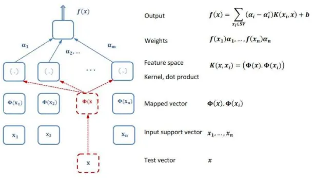
The architecture of a regression machine is depicted graphically in Figure 7, with the different steps for support vector algorithm. The input of the support vector for training processes is mapped
into a feature space by a map . Evaluation of kernel step is processed with a dot product of the
training data under the map (Smola and Schölkopf, 2004). The feature space for nonlinear
func-Latin A m erican Journal of Solids and Structures 12 (2015) 271-294
tions are based on the variance-covariance, a polynomial, radial basis function (RBF), polynomial of
degree , Gaussian RBF network, splines (Sánchez A., 2003). The output prediction in the feature
space is obtained with the weights and the term b as in Eq. (22). This support vector
machine constructs the decision function in learning machine process. After the training steps are concluded, a test vector is applied in order to verify the results and validate the metamodel. In order to check the results, the correlation factor R2 is computed (Meyers and Montgomery, 2002, Reddy et al., 2011) as
(24)
where are the targets or experimental values and are the outputs or predicted values from
SVR. This regression coefficient estimates the correlation between SVR predicted values and tar-get values.
Latin A m erican Journal of Solids and Structures 12 (2015) 271-294
4 NUMERICAL RESULTS
The laminated structure analyzed here is taken from the work of Varelis and Saravanos (2004). Figure 8 shows its geometry and engineering properties.
Figure 8: Geometry and properties of the laminated composite plate.
As already mentioned, the Latin hypercube scheme is used to define the samples. Data samples are different stacking sequence laminates for which the buckling load is computed in order to provide the input-output training pairs for the metamodels. The buckling load is obtained using the com-mercial finite element package Abaqus. A neural network metamodel and a support vector machine metamodel are trained, and their performances are compared.
4.1 Latin hypercube sampling data
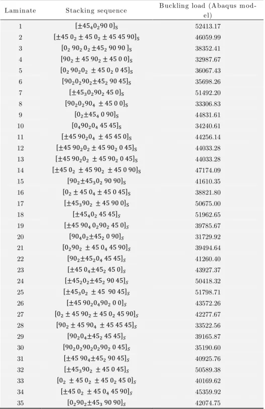
LH plan is applied to select representative stacking sequences of symmetrical laminates with 24
layers and discrete angles . The following stacking sequence is assumed
,. As we can observe, the laminate is not balanced and we have 7
variables. 120 laminates are generated by LHS, and their buckling loads are computed by a nu-merical model built in the finite element package Abaqus. Then, as a first attempt, 35 sampling points (laminates) were selected for the training step for both metamodels. These quantities are
based on the studies of Pan et al. (2010) and Yang and Gu (2004). They used 5 , where is
the total number of design variables. Table 2 presents the 35 samplings of laminates selected,
con-sidering , to train the metamodel and the corresponding buckling loads obtained via finite
Latin A m erican Journal of Solids and Structures 12 (2015) 271-294
Latin hypercube training sam ples and the corresponding responses
Lam inate Stacking sequence Buckling load (A baqus m
od-el)
1 52413.17
2 46059.99
3 38352.41
4 32987.67
5 36067.43
6 35698.26
7 51492.20
8 33306.83
9 44831.61
10 34240.61
11 44256.14
12 44033.28
13 44033.28
14 47174.09
15 41610.35
16 38821.80
17 50675.00
18 51962.65
19 39785.67
20 31729.92
21 39494.64
22 41260.40
23 43927.37
24 50418.32
25 51798.71
26 43572.26
27 42277.67
28 33522.56
29 39165.87
30 35190.60
31 40925.76
32 50589.38
33 40169.62
34 45359.92
35 42074.75
Latin A m erican Journal of Solids and Structures 12 (2015) 271-294
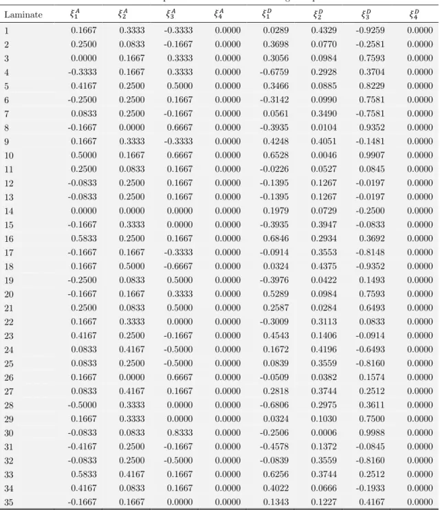
The pairs of laminate angular orientation and corresponding buckling loads may be converted in pairs of lamination parameters and corresponding buckling loads, as exposed in section 2.1. The advantage of doing this is that the number of lamination parameters is constant. This means that, for metamodels training purposes, the number of inputs became constant. The lamination parame-ters are computed with Eq. (7) and the results are shown in Table 3.
Lam ination param eters for the training sam ples
Laminate
1 0.1667 0.3333 -0.3333 0.0000 0.0289 0.4329 -0.9259 0.0000
2 0.2500 0.0833 -0.1667 0.0000 0.3698 0.0770 -0.2581 0.0000
3 0.0000 0.1667 0.3333 0.0000 0.3056 0.0984 0.7593 0.0000
4 -0.3333 0.1667 0.3333 0.0000 -0.6759 0.2928 0.3704 0.0000
5 0.4167 0.2500 0.5000 0.0000 0.3466 0.0885 0.8229 0.0000
6 -0.2500 0.2500 0.1667 0.0000 -0.3142 0.0990 0.7581 0.0000
7 0.0833 0.2500 -0.1667 0.0000 0.0561 0.3490 -0.7581 0.0000
8 -0.1667 0.0000 0.6667 0.0000 -0.3935 0.0104 0.9352 0.0000
9 0.1667 0.3333 -0.3333 0.0000 0.4248 0.4051 -0.1481 0.0000
10 0.5000 0.1667 0.6667 0.0000 0.6528 0.0046 0.9907 0.0000
11 0.2500 0.0833 0.1667 0.0000 -0.0226 0.0527 0.0845 0.0000
12 -0.0833 0.2500 0.1667 0.0000 -0.1395 0.1267 -0.0197 0.0000
13 -0.0833 0.2500 0.1667 0.0000 -0.1395 0.1267 -0.0197 0.0000
14 0.0000 0.0000 0.0000 0.0000 0.1979 0.0729 -0.2500 0.0000
15 -0.1667 0.3333 0.0000 0.0000 -0.3935 0.3947 -0.0833 0.0000
16 0.5833 0.2500 0.1667 0.0000 0.6846 0.2934 0.3692 0.0000
17 -0.1667 0.1667 -0.3333 0.0000 -0.0914 0.3553 -0.8148 0.0000
18 0.1667 0.5000 -0.6667 0.0000 0.0324 0.4375 -0.9352 0.0000
19 -0.2500 0.0833 0.5000 0.0000 -0.3976 0.0422 0.1493 0.0000
20 -0.1667 0.1667 0.3333 0.0000 0.5289 0.0984 0.7593 0.0000
21 0.2500 0.0833 0.5000 0.0000 0.2587 0.0284 0.6493 0.0000
22 0.1667 0.3333 0.0000 0.0000 -0.3009 0.3113 0.0833 0.0000
23 0.4167 0.2500 -0.1667 0.0000 0.4543 0.1406 -0.0914 0.0000
24 0.0833 0.4167 -0.5000 0.0000 0.1672 0.4196 -0.6493 0.0000
25 0.0833 0.2500 -0.5000 0.0000 0.0839 0.3559 -0.8160 0.0000
26 0.1667 0.0000 0.6667 0.0000 -0.0509 0.0382 0.1574 0.0000
27 0.0833 0.4167 0.1667 0.0000 0.2818 0.3744 0.2512 0.0000
28 -0.5000 0.3333 0.0000 0.0000 -0.6806 0.2975 0.3611 0.0000
29 0.1667 0.3333 0.0000 0.0000 0.0324 0.1030 0.7500 0.0000
30 -0.0833 0.0833 0.8333 0.0000 -0.2506 0.0006 0.9988 0.0000
31 -0.4167 0.2500 -0.1667 0.0000 -0.4578 0.1372 -0.0845 0.0000
32 -0.0833 0.2500 -0.5000 0.0000 -0.0839 0.3559 -0.8160 0.0000
33 0.5833 0.4167 0.1667 0.0000 0.6256 0.3744 0.2512 0.0000
34 0.4167 0.0833 0.1667 0.0000 0.4022 0.0666 -0.1933 0.0000
35 -0.1667 0.1667 0.0000 0.0000 0.1343 0.1227 0.4167 0.0000
Latin A m erican Journal of Solids and Structures 12 (2015) 271-294
4.2 Support Vector Regression Metamodel
A support vector regression script was developed in Python language. The input data generated from Latin hypercube is the computational experiments matrix with 35 stacking sequences, convert-ed to lamination parameters, as shown in Table 3. Gaussian RBF function was adoptconvert-ed as the ker-nel function. The simulation of training data sampling with Latin hypercube sampling and buckling load is presented in Figure 9.
Figure 9: Results from SVR metamodel.
Latin A m erican Journal of Solids and Structures 12 (2015) 271-294 Latin hypercube training samples and the corresponding responses
Laminate Stacking sequence Buckling load
1 45545.04
2 32924.13
3 37879.82
4 53369.56
5 43153.43
6 44933.25
7 44237.63
8 44237.63
9 48430.77
10 30251.10
11 45477.40
12 45850.84
13 38248.11
14 32989.45
15 52232.50
Table 4: Validated sampling by LH for laminated composites.
Latin A m erican Journal of Solids and Structures 12 (2015) 271-294
4.3 Neural Network Metamodel
In this work, the neural network is trained using the Matlab Neural Network Toolbox (MATLAB, 2010). In order to compare neural network and SVR results, the training data are the same for both metamodels. NN uses a network with one hidden layer with 10 neurons. The neural network train-ing results are presented in Figure 11. This figure shows a comparison between neural network out-puts and target outout-puts. It is possible to see that the neural network is well trained, which is con-firmed by the linear regression with a correlation factor equal to 1.
Figure 11: Results from NN metamodel.
Latin A m erican Journal of Solids and Structures 12 (2015) 271-294 Figure 12: Validated results from NN metamodel.
Latin A m erican Journal of Solids and Structures 12 (2015) 271-294
The results showed that the neural network needs more training pairs to learn the behavior of the system. The reasons why the SVR had a better performance than NN can be in the radial basis function used by SVR as kernel functions. This function returned a better nonlinear regression than a neural network approximation. Neural network is based on the Empirical Risk Minimization Inductive Principle. This principle approximates responses for large samples. On the other hand, SVR applies the Structural Risk Minimization Inductive Principle that is based on subset of sam-ples. Vapnik (2000) presented this approach and applied the statistic learning theory. Furthermore, the fact that SVR optimality is rooted in convex optimization and neural network in minimizing the errors by the backpropagation algorithm can also explain the results.
Besides the application of SVR and NN metamodels, another contribution of this work was the use of lamination parameters as inputs for the metamodels instead of angular ply orientations for a composite structure analysis. This makes possible to use the same metamodel for representing a laminate with a different number of layers. This means that the metamodels trained with input-output pairs representing a 24-layer laminate can be used for laminates with different number of layers, once the total thickness remains the same.
5 CONCLUSIONS
Latin A m erican Journal of Solids and Structures 12 (2015) 271-294
References
Arnold, R.R., Mayers, J. (1984). Buckling, postbuckling, and crippling of materially nonlinear laminated composite plates, Int. J. Solids Structures 20:863-880.
Baba, B.O. (2007). Buckling behavior of laminated composite plates, Journal of Reinforced Plastics and Composites 26:1637-1655.
Basak, D., Pal, S., Patranabis, D.C. (2007). Support Vector Regression, Neural Information Processing – Letters and Reviews 11:203-224.
Ben-Hur, A., Horn, D., Siegelmann, H.T., Vapnik, V. (2001). Support Vector Clustering, Journal of Machine Learn-ing Research 2:125-137.
Bezerra, E.M., Ancelotti, A.C., Pardini, L.C., Rocco, J.A.F.F., Iha, K., Ribeiro, C.H.C. (2007). Artificial neural networks applied to epoxy composites reinforced with carbon and E-glass fibers: Analysis of the shear mechanical properties, Materials Science & Engineering A 464:177-185.
Boser, B.E., Guyon, I.M., Vapnik, V. (1992). A training algorithm for optimal margin classifiers, Association for Computing Machinery, 7:144-152.
Che, J. (2013). Support vector regression based on optimal training subset and adaptive particle swarm optimization algorithm, Applied Soft Computing 13:3473-3481.
Cheng, J., Druzdzel, M.J. (2000). Latin hypercube sampling in bayesian networks, In Proceedings of FLAIRS-2000-AAAI 2000, Orlando, USA.
Erdal, O., Sonmez, F.O. (2005). Optimum design of composite laminates for maximum buckling load capacity using simulated annealing, Composite Structures 71:45-52.
Forrester, A.I.J., Sóbester, F. and Keane, A.J., (2008). Engineering design via surrogate modeling: a practical guide, John Wiley & Sons (United Kingdom).
Foldager, J., Hansen, J. S., Olhoff, N. (1998). A general approach forcing convexity of ply angle optimization in composite laminates, Structural Optimization 16: 201-211.
Geier, B., Meyer-Piening, H.R., Zimmermann, R. (2002). On the influence of laminate stacking on buckling of com-posite cylindrical shells subjected to axial compression, Comcom-posite Structures 55:467-474.
Guo, G., Zhang, J. (2007). Reducing examples to accelerate support vector regression, Pattern Recognition Letters 28:2173-2183.
Hagan, M.T., Demuth, H. B. and Beale, M., (1996). Neural network design. PWS Pub., (Boston). Haykin, S., (1999). Neural Networks: A comprehensive foundation. Prentice-Hall, 2nd edition (New Jersey).
Herencia, J.E., Weaver, P. M., Friswell, M. I. (2007). Optimization of long anisotropic laminated fiber composite panels with T-shaped stiffeners, AIAA Journal 45:2497-2509.
Janouchova, E., Kucerova, A. (2013). Competitive comparison of optimal designs of experiments for sampling-based sensitivity analysis, Computers & Structures 124:47-60.
Jones, R.M., (1999). Mechanics of composite material, Taylor& Francis, 2nd edition(Philadelphia).
Kalnins, K., Jekabsons, G., Rikardis, R. (2009). Metamodels for optimisation of post-buckling responses in full-scale composite structures, In 8th World Congress on Structural and Multidisciplinary Optimization, Lisbon, Portugal. Leissa, A.W. (1993). Buckling of composite plates, Composite Structures 1:51-66.
Levenberg, K. (1944). A method for the solution of certain non-linear problems in least squares. Quartely of Applied Mathematics 2: 164-168.
Liao, X., Li, Q., Yang, X., Zhang, W., Li, W. (2008). Multiobjective optimization for crash safety design of vehicles stepwise regression model, Struct Multidisc Optim 35:561-569.
Latin A m erican Journal of Solids and Structures 12 (2015) 271-294 MATLAB Reference Guide (2010). The Math Works Inc
Mendonça, P.T., (2005). Materiais compostos e estruturas-sanduíche: projeto e análise (in Portuguese), Manole, 1st edition (Barueri).
Myers, R.H. and Montgomery, D., (2002). Response surface methodology: processes and product optimization using designed experiments, Wiley Interscience, 2nd edition (New York).
Pan, F., Zhu, P., Zhang, Y. (2010). Metamodel-based lightweight design of B-pillar with TWB structure via support vector regression, Computers and Structures 88:36-44.
Reddy, A.R., Reddy, B.S., Reddy, K.V.K. (2011). Application of design of experiments and artificial neural networks for stacking sequence optimization of laminated composite plates, International Journal of Engineering, Science and Technology 3:295-310.
Reddy, M.R.S., Reddy, B.S., Reddy, V.N., Sreenivasulu, S. (2012). Prediction of natural frequency of laminated composite plates using artificial neural networks, Engineering 4:329-337.
Sánchez A., V.D. (2003). Advanced support vector machines and kernel methods, Neurocomputing 55:5-20.
Shukla, K.K., Nath, Y., Kreuzer, E., Sateesh Kumar, K.V. (2005). Buckling of laminated composite rectangular plates, Journal of aerospace engineering 18:215-223.
Simpson, T.W., Toropov, V., Balabanov, V., Viana, F.A.C. (2008). Design and analysis of computer experiments in multidisciplinary design optimization: A review of how far we have come – or not, In 12th AIAAISSMO Multidisci-plinary Analysis and Optimization Conference, Victoria, Canada.
Smola, A.J., Schölkopf, B. (2004). A tutorial on support vector regression, Statistics and Computing 14: 199-222. Staab, G.H., (1999). Laminar Composite, Butterworth-Heinemann (Worbun).
Starnes, J.H., Knight, N.F., Rouse, M. (1985). Postbuckling behavior of selected flat stiffened graphite-epoxy panels loaded in compression, AIAA Journal 23:1236-1246.
Sundaresan, P., Singh, G., Rao, G. V. (1996). Buckling and post-buckling analysis of moderately thick laminated rectangular plates, Computers & Structures 61:79-86.
Suttorp, T., Igel, C. (2006). Multi-objective optimization of support vector machines, Multi-objective Machine Learn-ing Studies in Computational Intelligence 16:199-220.
Tsai, S.W., Pagano, N.J. (1968). Invariant properties of composite materials, In Composite Materials Workshop, Techno-mic, Stamford, Connecticut, 233-253.
Todoroki, A., Shinoda, T., Mizutani, Y.,Matsuzaki, R. (2011). New surrogate model to predict fracture of laminated CFRP for structural optimization, Journal of Computational Science and Technology 5:26-37.
Üstün, B., Melssen, W.J., Buydens, L.M.C. (2007). Visualisation and interpretation of support vector regression models, Analytica Chimica Acta 595:299-309.
Vapnik, V. (1993).Three fundamental concepts of the capacity of learning machines, Physica A 200:538-544. Vapnik, V. (1999). An overview of statistical learning theory, IEEE Transactions on Neural Networks 10:988-999. Vapnik, V.N., (2000). The nature of statistical learning theory. Springer-Verlag, 2nd edition (New York).
Vapnik, V., Vashist, A. (2009). A new learning paradigm: Learning using privileged information, Neural Networks 22:544-557.
Varelis, D., Saravanos, D.A. (2004). Coupled buckling and postbuckling analysis of active laminated piezoelectric composite plates, International Journal of Solids and Structures 41: 1519-1538.
Wang, W., Guo, S., Chang, N., Yang, W. (2010). Optimum buckling design of composite stiffened panels using ant colony algorithm, Composite Structures 92:712-719.
Wang, G.G., Shan, S. (2007). Review of metamodeling techniques in support of engineering design optimization, ASME Transactions, Journal of Mechanical design 129:370-380.