Sparse and compositionally robust inference of microbial ecological networks.

Sparse and Compositionally Robust Inference

of Microbial Ecological Networks

Zachary D. Kurtz1☯, Christian L. Müller2,3☯, Emily R. Miraldi1,2,3☯, Dan R. Littman1, Martin J. Blaser1, Richard A. Bonneau2,3,4*

1Departments of Microbiology and Medicine, New York University School of Medicine, New York, New York, United States of America,2Department of Biology, Center for Genomics and Systems Biology, New York University, New York, New York, United States of America,3Courant Institute of Mathematical Sciences, New York University, New York, New York, United States of America,4Simons Center for Data Analysis, Simons Foundation, New York, New York, United States of America

☯These authors contributed equally to this work. *rb133@nyu.edu

Abstract

16S ribosomal RNA (rRNA) gene and other environmental sequencing techniques provide snapshots of microbial communities, revealing phylogeny and the abundances of microbial populations across diverse ecosystems. While changes in microbial community structure are demonstrably associated with certain environmental conditions (from metabolic and im-munological health in mammals to ecological stability in soils and oceans), identification of underlying mechanisms requires new statistical tools, as these datasets present several technical challenges. First, the abundances of microbial operational taxonomic units (OTUs) from amplicon-based datasets are compositional. Counts are normalized to the total number of counts in the sample. Thus, microbial abundances are not independent, and traditional statistical metrics (e.g., correlation) for the detection of OTU-OTU relationships can lead to spurious results. Secondly, microbial sequencing-based studies typically mea-sure hundreds of OTUs on only tens to hundreds of samples; thus, inference of OTU-OTU association networks is severely under-powered, and additional information (or assump-tions) are required for accurate inference. Here, we present SPIEC-EASI (SParseInversE Covariance Estimation forEcologicalAssociationInference), a statistical method for the in-ference of microbial ecological networks from amplicon sequencing datasets that ad-dresses both of these issues. SPIEC-EASI combines data transformations developed for compositional data analysis with a graphical model inference framework that assumes the underlying ecological association network is sparse. To reconstruct the network, SPIEC-EASI relies on algorithms for sparse neighborhood and inverse covariance selection. To provide a synthetic benchmark in the absence of an experimentally validated gold-standard network, SPIEC-EASI is accompanied by a set of computational tools to generate OTU count data from a set of diverse underlying network topologies. SPIEC-EASI outperforms state-of-the-art methods to recover edges and network properties on synthetic data under a variety of scenarios. SPIEC-EASI also reproducibly predicts previously unknown microbial associations using data from the American Gut project.

a11111

OPEN ACCESS

Citation:Kurtz ZD, Müller CL, Miraldi ER, Littman DR, Blaser MJ, Bonneau RA (2015) Sparse and Compositionally Robust Inference of Microbial Ecological Networks. PLoS Comput Biol 11(5): e1004226. doi:10.1371/journal.pcbi.1004226

Editor:Christian von Mering, University of Zurich and Swiss Institute of Bioinformatics, SWITZERLAND

Received:August 19, 2014

Accepted:March 2, 2015

Published:May 7, 2015

Copyright:© 2015 Kurtz et al. This is an open access article distributed under the terms of the

Creative Commons Attribution License, which permits unrestricted use, distribution, and reproduction in any medium, provided the original author and source are credited.

Data Availability Statement:All code and data are available fromhttp://bonneaulab.bio.nyu.edu/

Funding:This work was supported by the National Institutes of Health grants T32AI007180-30 (ZDK, ERM), R01 DK103358-01 (DRL, RAB) and RO1 GM63270 (MJB) and the Simons Foundation (CLM, ERM, RAB). The funders had no role in study design, data collection and analysis, decision to publish, or preparation of the manuscript.

Author Summary

Genomic survey of microbes by 16S rRNA gene sequencing and metagenomics has in-spired appreciation for the role of complex communities in diverse ecosystems. However, due to the unique properties of community composition data, standard data analysis tools are likely to produce statistical artifacts. For a typical experiment studying microbial eco-systems these artifacts can lead to erroneous conclusions about patterns of associations be-tween microbial taxa. We developed a new procedure that seeks to infer ecological

associations between microbial populations, by 1) taking advantage of the proportionality invariance of relative abundance data and 2) making assumptions about the underlying network structure when the number of taxa in the dataset is larger than the number of sampled communities. Additionally, we employed a novel tool to generate biologically plausible synthetic data and objectively benchmark current association inference tools. Fi-nally, we tested our procedures on a large-scale 16S rRNA gene sequencing dataset sam-pled from the human gut.

Introduction

Low-cost metagenomic and amplicon-based sequencing promises to make the resolution of complex interactions between microbial populations and their surrounding environment a routine component of observational ecology and experimental biology. Indeed, large-scale data collection efforts (such as Earth Microbiome Project [1], the Human Microbiome Project [2], and the American Gut Project [3]) bring an ever-increasing number of samples from soil, ma-rine and animal-associated microbiota to the public domain. Recent research efforts in ecology, statistics, and computational biology have been aimed at reliably inferring novel biological in-sights and testable hypotheses from population abundances and phylogenies. Classic objectives in community ecology include, (i) the accurate estimation of the number of taxa (observed and unobserved) from microbial studies [4] and, related to that, (ii) the estimation of community diversity within and across different habitats from the modeled population counts [5]. More-over, some microbial compositions appear to form distinct clusters, leading to the concept of enterotypes, or ecological steady states in the gut [6], but their existence has not been estab-lished with certainty [7]. Another aim of recent studies is the elucidation of connections be-tween microbes and environmental or host covariates. Examples include a novel statistical regression framework for relating microbiome compositions and covariates in the context of nutrient intake [8], observations that microbiome compositions strongly correlate with disease status in new-onset Crohn’s disease [9], and the connections between helminth infection and the microbiome diversity [10].

network is correlation analysis; that is computing Pearson’s correlation coefficient among all pairs of OTU samples, and an interaction between microbes is assumed when the absolute value of the correlation coefficient is sufficiently high [15,16].

However, applying traditional correlation analysis to amplicon surveys of microbial popula-tion data is likely to yield spurious results [9,17]. To limit experimental biases due to sampling depth, OTU count data is typically transformed by normalizing each OTU count to the total sum of counts in the sample. Thus, communities of microbial relative abundances, termed compositions, are not independent, and classical correlation analysis may fail [18]. Recent methods such as Sparse Correlations for Compositional data (SparCC) [17] and Composition-ally Corrected by REnormalization and PErmutation (CCREPE) [9,11,19] are designed to ac-count for these compositional biases and represent the state of the art in the field. Yet, it is not clear that correlation is the proper measure of association. For example, correlations can arise between OTUs that are indirectly connected in an ecological network (we expand on this point below).

Dimensionality poses another challenge to statistical analysis of microbiome studies, as the number of measured OTUspis on the order of hundreds to thousands whereas the number of samplesngenerally ranges from tens to hundreds. This implies that any meaningful interaction inference scheme must operate in the underdetermined data regime (p>n), which is viable only if additional assumptions about the interaction network can be made. As technological de-velopments lead to greater sequencing depths, new computational methods that address the (p>n) challenge will become increasingly important.

In the present work, we present a novel strategy to infer networks from (potentially high-di-mensional) community composition data. We introduce SPIEC-EASI (SParseInversE C ovari-ance Estimation forEcologicalASsociationInference, pronouncedspeakeasy), a new statistical method for the inference of microbial ecological networks and generation of realistic synthetic data. SPIEC-EASI inference comprises two steps: First, a transformation from the field of com-positional data analysis is applied to the OTU data. Second, SPIEC-EASI estimates the interac-tion graph from the transformed data using one of two methods: (i) neighborhood selecinterac-tion [20,21] and (ii) sparse inverse covariance selection [22,23]. Unlike empirical correlation or co-variance estimation, used in SparCC and CCREPE, our pipeline seeks to infer an underlying graphical model using the concept of conditional independence.

Informally, two nodes (e.g. OTUs) are conditionally independent if, given the state (e.g. abundance) of all other nodes in the network, neither node provides additional information about the state of the other. A link between any two nodes in the graphical model implies that the OTU abundances are not conditionally independent and that there is a (linear) relationship between them that cannot be better explained by an alternate network wiring. In this way, our method avoids detection of correlated but indirectly connected OTUs, thus ensuring parsimo-ny of the resulting network model (for more detail, seeMaterials and MethodsandFig 1). This model is an undirected graph where links between nodes represent signed associations between OTUs. The use of graphical models has gained considerable popularity in network biology [24–26] and, more recently, in structural biology [27], particularly to correct for transitive cor-relations in protein structure prediction [28].

high-dimensional statistics [29–31] suggests that network topology can strongly impact network re-covery and performance and thus must be considered in the design of synthetic datasets.

We show that SPIEC-EASI is a scalable inference engine that (i) yields superior performance with respect to state-of-the-art methods in terms of interaction recovery and network features in a diverse set of realistic synthetic benchmark scenarios, (ii) provides the most stable and re-producible network when applied to real data, and (iii) reliably estimates an invertible covari-ance matrix which can be used for additional downstream statistical analysis. In agreement with statistical theory [29], inference on the synthetic datasets demonstrates that the degree distribu-tion of the underlying network has the largest effect on performance, and this effect is observed across all methods tested. SPIEC-EASI network inference applied to actual data from the Ameri-can Gut Project (AGP) shows (i) that clusters of strongly connected components are likely to contain OTUs with common family membership and (ii) that actual gut microbial networks are likely composites of archetypical network topologies. In the Materials and Methods section, we present statistical and computational aspects of SPIEC-EASI. We then benchmark SPIEC-EASI, comparing it to current inference schemes using synthetic data. We then apply SPIEC-EASI to measurements available from the AGP database. The SPIEC-EASI pipeline is implemented in the R package [SpiecEasi] freely available athttps://github.com/zdk123/SpiecEasi. All presented numerical data is available athttp://bonneaulab.bio.nyu.edu/.

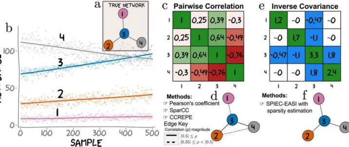
Fig 1. Conditional independence vs correlation analysis for a toy dataset.In an ecosystem, the abundance of any OTU is potentially dependent on the abundances of other OTUs in the ecological network. Here, we simulate abundances from a network where OTU 3 directly influences (via some set of biological mechanisms) the abundances of OTUs 1, 2 and 4 (a). The inference goal here is to recover the underlying network from the simulated data.b) Absolute abundances of these four OTUs were drawn from a negative-binomial distribution across 500 samples according to the true network (as described in the Methods section).c) Computing all pairwise Pearson correlation yields a symmetric matrix showing patterns of association (positive correlations are green and negative are red). We thresholded entries of the correlation matrix to generate relevance networks.d) A threshold atρ _j0.35j(represented by dashed and solid edges) results in a network in which OTU 3 is connected to all other OTUs with an additional connection between OTU 2 and OTU 4. A more stringent threshold atρ j0.5j, results in a sparser relevance network (notably missing the edge between OTU 3 and OTU 1), and is represented ind

by solid edges only. Importantly, no single threshold recovers the true underlying hub topology.e) The inverse sample covariance matrix yields a symmetric matrix where entries are approximately zero if the corresponding OTU pairs are conditionally independent. The network (f) inferred from the non-zero entries (colored in blue ine) identifies the correct hub network. Thus, it is possible to choose a threshold for the sample inverse covariance that faithfully recovers the true network. Such a threshold is not guaranteed to exist for correlation or covariance (the metric used by SparCC and CCREPE). Intuitively, this is because simultaneous direct connections can induce strong correlations between nodes that do not have direct relationships (e.g. OTU 2-4). Conversely, weak correlations can arise between directly connected nodes (e.g. OTU 1-3). Although correlation is a useful measure of association in many contexts, it is a pairwise metric and therefore limited in a multivariate setting. On the other hand, SPIEC-EASI’s estimate of entries in the inverse covariance matrix depend on the conditional states of all available nodes. This feature helps SPIEC-EASI avoid detection of indirect network interactions.

Materials and Methods

SPIEC-EASI comprises both an inference and a synthetic data generation module.Fig 2 sum-marizes the key components of the pipeline. In this section, we introduce all statistical and computational aspects of the inference scheme and then describe our approach for generating realistic synthetic datasets.

Data processing and transformation of standard OTU count data

For this discussion, a table of OTU count data, typical output of 16S rRNA gene sequencing data curation pipelines (e.g., mothur [32], QIIME [33]) are given. The OTU data are stored in a matrixW₂Nnp

0 wherewðjÞ¼ ½w

ðjÞ

1 ;w

ðjÞ

2 ;. . .;wðjÞp Šdenotes thep-dimensional row vector of

OTU counts from thejthsample,j= 1,. . .,n, with total cumulative countmðjÞ _¼P

p

i¼1

wðjÞi ;N0

de-notes the set of natural numbers {0, 1, 2,. . .}. As described above, to account for sampling bi-ases, microbiome data is typically transformed by normalizing the raw count dataw(j)with respect to the total countm(j)of the sample [10]. We thus arrive at vectors of relative

abun-dances or compositionsxðjÞ_{¼ ½}wðjÞ1

mðjÞ;

wðjÞ₂ mðjÞ;. . .;

wðpjÞ

mðjފfor samplej. Due to this normalization OTU

abundances are no longer independent, and the sample space of this p-part compositionx(j)is not the unconstrained Euclidean space but thep-dimensional unit simplex

Sp_¼:_{fx jx}

i>0;

Pp

i¼1xi¼1g. Thus, OTU compositions from n samples are constrained to lie

in the unit simplex, X2Sn×p_{. This restriction of the data to the simplex prohibits the}

applica-tion of standard statistical analysis techniques, such as linear regression or empirical covariance estimation. Covariance matrices of compositional data exhibit, for instance, a negative bias due to closure effects.

Major advances in the statistical analysis of compositional data were achieved by Aitchison in the 1980’s [18,34]. Rather than considering compositions in the simplex, Aitchison pro-posed log-ratios, log½xi

xjŠ, as a basis for studying compositional data. The simple equivalence

log½xi

xjŠ ¼log½

wi=m

wj=mŠ ¼log½

wi

wjŠimplies that statistical inferences drawn from analysis of log-ratios

of compositions are equivalent to those that could be drawn from the log-ratios of the unob-served absolute measurements, also termed thebasis.

Aitchison also proposed several statistically equivalent log-ratio transformations to remove the unit-sum constraint of compositional data [18]. Here we apply the centered log-ratio (clr) transform:

z ¼: clrðxÞ ¼ ½logðx1=gðxÞÞ;. . .;logðxp=gðxފ ¼ ½logðw1=gðwÞÞ;. . .;logðwp=gðwÞފ ð1Þ

wheregðxÞ ¼ Qp

i¼1 xi

1=p

is the geometric mean of the composition vector. The clr transform is

symmetric and isometric with respect to the component parts. The resulting vectorzis con-strained to a zero sum. The clr transform maps the data from the unit simplex to ap−

1-dimen-sional Euclidean space, and the corresponding population covariance matrixΓ_{= Cov[clr(X)]2}

Rp×p_{is also singular [18]. The covariance matrix}Γ_{is related to the population covariance of}

the log-transformed absolute abundancesO_{= Cov[logW] via the relationship [34]:}

G_¼GO_{G ð2Þ}

whereG_¼I_p 1

pJ, Ipis thep-dimensional identity matrix, and J = [j1,j2,. . .,ji,. . .,jp],ji=

G is close to the identity matrix, and thus we can assume that afinite sample estimatorG

^

_ofΓ serves as a good approximation ofO

^

_{. This approximation serves as the basis of our network} in-ference scheme. Finally, because real-world OTU data often contain samples with a zero count for low-abundance OTUs, we add a unit pseudo count to the original count data to avoid nu-merical problems with the clr transform.

Inference of microbial associations from microbial abundance datasets

Our key objective is to learn a network of pairwise taxon-taxon associations (putative interac-tions) from clr-transformed microbiome compositionsZ2Rn×p_{. We represent the network as}

an undirected, weighted graphG_{= (V,E), where the vertex setV= {v1,}. . .,vp} represents thep

taxa (e.g., OTUs) and the edge setEV×Vthe possible associations among them. Our formal approach is to learn a probabilistic graphical model [35] (i) that is consistent with the observed data and (ii) for which the (unknown) graphG_{encodes the conditional dependence structure}

between the random variables (in our case, the observed taxa). Graphical models over undirect-ed graphs (also known as Markov networks or Markov Random Fields) have a straightforward distributional interpretation when the data are drawn from a probability distributionπ(x) that

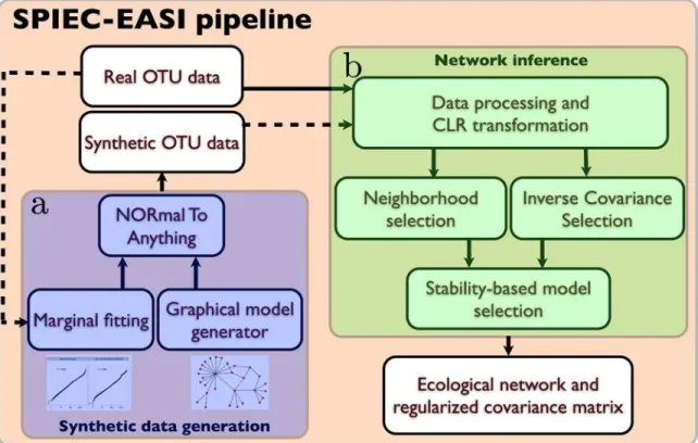
Fig 2. Workflow of the SPIEC-EASI pipeline.The SPIEC-EASI pipeline consists of two independent parts fora) synthetic data generation andb) network inference.a) Synthetic data generation requires an OTU count table and a user-selected network topology. Internally, the parameters of a statistical distribution (the zero-inflated Negative binomial model is suggested) are fit to the OTU marginals of the real data, and are combined with the randomly-generated network in the Normal to Anything (NORTA) approach to generate correlated count data.b) Network inference proceeds in three stages on synthetic or real OTU count data: First, data is pre-procssed and centered log-ratio (CLR) transformed to ensure compositional robustness. Next, the user selects one of two graphical model inference procedures: 1) Neighborhood selection (the MB method) or 2) inverse covariance selection (the glasso method). SPIEC-EASI network inference assumes that the underlying network is sparse. We infer the correct model sparseness by the Stability Approach to Regularization Selection (StARS), which involves random subsampling of the dataset to find a network with low variability in the selected set of edges. SPIEC-EASI outputs include an ecological network (from the non-zero entries of the inverse covariance network) and an invertible covariance matrix. If the network was inferred from synthetic data, it can be compared with the input network to assess inference quality.

belongs to an exponential family [36,37]. For example, when the data are drawn from a multi-variate normal distributionπ(x) =N_(xjμ,S_{) with meanμand covariance}S_{, the non-zero} ele-ments of the off-diagonal entries of the inverse covariance matrixΘ₌S−1_{, also termed the}

precision matrix, defines the adjacency matrix of the graphG_{and thus describes the}

factoriza-tion of the normal distribufactoriza-tion into condifactoriza-tionally dependent components [35]. Conversely, if and only if an entry inΘ_:Θ

i,j= 0, then the two variables are conditionally independent, and

there is no edge betweenviandvjinG. We seek to estimate the inverse covariance matrix from

the data, thereby inferring associations based on conditional independence. This is fundamen-tally distinct from SparCC and CCREPE (seeS1 Table), which essentially estimate pairwise correlations (though other pairwise metrics could be considered for CCREPE). We highlight this key difference inFig 1. For an intuitive introduction to graphical models in the context of biological networks see Bühlmannet. al, 2014 [38].

Inferring the exact underlying graph structure in the presence of a finite amount of samples is, in general, intractable. However, two types of statistical inference procedures have been use-ful in high-dimensional statistics due to their provable performance guarantees under assump-tions about the sample sizen, dimensionalityp, underlying graph properties, and the

generating distribution [29,39]. The first approach, neighborhood selection [20,39], aims at reconstructing the graph on a node-by-node basis where, for each node, a penalized regression problem is solved. The second approach is the penalized maximum likelihood method [22,23], where the entire graph is reconstructed by solving a global optimization problem, the so-called covariance selection problem [40]. The key advantages of these approaches are that (i) their un-derlying inference procedures can be formulated as convex (and hence tractable) optimization problems, and (ii) they are applicable even in the underdetermined regime (p>n), provided that certain structural assumptions about the underlying graph hold. One assumption is that the true underlying graph is reasonably sparse, e.g., that the number of taxon-taxon associa-tions scales linearly with the number of measured taxa.

Graphical model inference. The SPIEC-EASI pipeline comprises two types of inference

schemes, neighborhood and covariance selection. The neighborhood selection framework, in-troduced byMeinshausen andBühlmann [20] and thus often referred as the MB method, tack-les graph inference by solvingpregularized linear regression problems, leading to local

conditional independence structure predictions for each node. Let us denote theithcolumn of the data matrixZbyZi2Rn_{and the remaining columns byZ}¬i₂Rn×p−1_{. For each nodevi, we}

solve the following convex problem:

^

bi;l_¼argmin b2Rp 1

1

nkZ

i _Z:i_bk2

þlkbk1

; _ð3Þ

wherekak1¼ Pp 1

i¼1 jaijdenotes the L1 norm, andλ0 is a scalar tuning parameter. This

so-called LASSO problem [41] aims at balancing the least-squarefit and the number of necessary predictors (the non-zero componentsβ_jofβ) by tuning theλ_{parameter. We define the local} neighborhood of a nodeviasNil¼ fj f1;. . .pg\i: ^b

i;l

j 6¼0g. Thefinal edge setEofGcan

be defined via the intersection or the union operation of the local neighborhoods. An edgeei,j

between nodeviandvjexists ifj2Nil\i2N

l

j orj2N

l

i [i2N

l

j. For edges in the set

j2Nl

i \i2N

l

j, the edge weights,ei,jandej,i, are estimated using the average of the two

The second inference approach, (inverse) covariance selection, relies on the following penal-ized maximum likelihood approach. In the standard Gaussian setting, the related convex opti-mization problem reads:

Y

^

_¼argmin Y_2PD ð

log detðY_{Þ þtrð}YS

^

_{Þ þ}lkY_k

1Þ; ð4Þ

where PD denotes the set of symmetric positive definite matrices {A:xTAx>0,8x2Rp_},S

^

the empirical covariance estimate,kk1the element-wise L1 norm, andλ0 a scalar tuning

parameter. Forλ= 0, the expression is identical to the maximum likelihood estimate of a nor-mal distributionN_(xj0,S_{). For non-zero}λ, the objective function (also referred as the graphi-cal Lasso [22]) encourages sparsity of the underlying precision matrixΘ_{. The non-zero,} off-diagonal entries inΘ_{define the adjacency matrix of the interaction graph}G_{which, similar to}

MB, depends on the proper choice of the penalty parameterλ. Originally, this estimator was shown to have theoretical guarantees on consistency and recovery only under normality as-sumptions [43]. However, recent theoretical [29,44] work shows that distributional assump-tions can be considerably relaxed, and the estimator is applicable to a larger class of problems, including inference on discrete (count) data. In addition, nonparametric approaches, such as sparse additive models, can be used to“gaussianize”the data prior to network inference [45]. We thus propose the following estimator for inferring microbial ecological associations. Given clr-transformed OTU dataZ2Rn×p_{, we propose the modified optimization problem:}

O

^

1

¼arg min

O 1_2PD

ð log detðO 1_{Þ þtrð}O 1G

^

_{Þ þlk}O 1_k

1Þ; ð5Þ

whereG

^

_{is the empirical covariance estimate ofZ, and}O−1_{is the inverse covariance (or}

preci-sion matrix) of the underlying (unknown) basis. As stated above,G

^

_{will be a good} approxima-tion for the basis covariance matrixO

^

_{becausep> >0. The resulting solution is constrained to} the set of PD matrices, ensuring that the penalized estimator has full rankp. The non-zero off-diagonal entries of the estimated matrixO−1

define the inferred networkG_{, and their values are}

the signed edge weights of the graph. To reduce the variance of the estimate, the covariance matrix

^

G_{can also be replaced by the empirical correlation matrixR}^_¼DG^_{D, whereDis a} diag-onal matrix that contains the inverse of the estimated element-wise standard deviations.

The covariance selection approach has two advantages over the neighborhood selection framework. First, we obtain unique weights associated with each edge in the network. No aver-aging or subsequent edge selection is necessary. Second, the covariance selection framework provides invertible precision and covariance matrix estimates that can be used in further down-stream microbiome analysis tasks, such as regression and discriminant analysis [10].

Model selection. For both neighborhood and covariance selection, the tuning parameter λ₂[0,λmax] controls the sparsity of the final model. Rather than inferring a single graphical

observed edge frequencies indicate the reproducibility, and likely the predictive power, and are used to rank edges according to confidence.

Theoretical and computational aspects. Learning microbial graphical models with

neigh-borhood or inverse covariance selection schemes has important theoretical and practical ad-vantages over current methods. A wealth of theoretical results are available that characterize conditions for asymptotic and finite sample guarantees for the estimated networks [20,29,39, 43,46]. Under certain model assumptions, the number of samplesnnecessary to infer the true topology of the graph in the neighborhood selection framework is known to scale asn=O(d3

log(p)), wheredis the maximum vertex (or node) degree of the underlying graph (i.e. the maxi-mum size of any local neighborhood). Additional assumptions on the sample covariance matri-ces reduce the scaling ton=O(d2log(p)) [39]. This implies that graph recovery and precision matrix estimation is indeed possible even in thep> >nregime, and that the underlying graph topology strongly impacts edge recovery. The latter observation means that, even if the number of interactionseis constant, graphs with large hub nodes, perhaps representing keystone spe-cies in microbial networks, or, more generally, scale-free graphs with, a few highly connected nodes, will be more difficult to recover than networks with evenly distributed neighborhoods. In addition to these theoretical results, a second advantage is that well-established, efficient, and scalable implementations are available to infer microbial ecological networks from OTU data in practice. Thus, SPIEC-EASI methods will efficiently scale as microbiome dataset di-mensions grow (e.g., due to technological advances that increase the number of OTUs detected per sample). The SPIEC-EASI inference engine relies on the R packagehuge[49], which in-cludes algorithms to solve neighborhood and covariance selection problems [20,22], as well as the StARS model selection.

Generation of synthetic microbial abundance datasets

Estimating the absolute and comparative performance of network inference schemes from bio-logical data remains a fundamental challenge in biology. In the context of gene regulatory net-work inference, recent community-wide efforts, such as the DREAM (Dialogue for Reverse Engineering Assessments and Methods) Challenges (http://www.the-dream-project.org/), have considerably advanced our understanding about feasibility, accuracy, and applicability of a large number of developed methods. In the DREAM challenges, both real data from“gold stan-dard”regulatory networks (e.g., networks where the true topology is known from independent experimental evidence) and realistic in-silico data (using, e.g., the GeneNetWeaver pipeline [50]) are included. In the context of microbiome data and microbial ecological networks, nei-ther a gold standard nor a realistic synthetic data generator exist. SPIEC-EASI is accompanied by a set of computational tools that allow the generation of realistic synthetic OTU data. As outlined inFig 2, real taxa count data serve as input to SPIEC-EASI’s synthetic data generation pipeline. The pipeline enables one to: (i) fit the marginal distributions of the count data to a parametric statistical model and (ii) specify the underlying graphical model architecture (e.g., scale-free).

The NorTA approach. The parametric statistical model and network topology are then

combined in the‘Normal To Anything’(NorTA) [51] approach to generate synthetic OTU data that resemble real measurements from microbial communities but with user-specified net-work topologies. NorTA [51] is an approximate technique to generate arbitrary continuous and discrete multivariate distributions, given (1) a target correlation structureRwith entries ρi,jand (2) a target univariate marginal distributionUi. To achieve this task, NorTA relies on

distribution with zero mean and ap×pcorrelation matrix RN. For each marginalUi, the

Nor-mal cumulative distribution function (CDF) is transformed to the target distribution via its in-verse CDF. For any target distributionPwith CDFX_{, we can thus generate multivariate} correlated data via

UPi ¼X 1

ðF_ðU

NiÞÞ; ð6Þ

where UN*N(0, RN) andFðUÞ ¼

R

U

1

1 ffiffiffiffiffi 2s2

p _e u

2

2 du, the CDF of a univariate normal. InFig 3a,

we illustrate this process for bivariate Poisson and negative binomial data (n= 1000 and corre-lationρij= 0.7).

In the original NorTA approach, an element-wise monotone transformationcU() with

RN=cU(R) is applied to account for slight differences in correlation structure between normal and target distribution samples [51]. Here we neglect this transformation step because we ob-serve that the log-transformed data from exponential count distributions, such as the Poisson and Negative binomial, are already close to R, provided that the mean is greater than one, par-ticularly when the counts data are log-transformed (S1 Fig). In practice, SPIEC-EASI relies on routines from base R and VGAM packages [54,55] to estimate the uniform quantiles of the normal data and to fit the desired CDF with estimated parameters.

Fitting marginal distribution to real OTU data. Prior to fitting marginal distributions to real data, several commonly used pre-proccesing steps are applied. For any given OTU abun-dance table of sizen×K, we first selectpnon-zero columns. To account for experimental

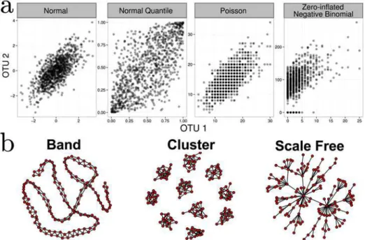
Fig 3. a)Bivariate illustration of the NorTA approach.First normal data, incorporating the target correlation structure, is generated. Uniform data are then generated for each margin via the normal density function. These is then converted to an arbitrary marginal distribution (Poisson and Zero-inflated Negative Binomial shown as examples) via its quantile function. To generate realistic synthetic data, parameters for these margins are fit to real data.b) Examples of band-like, cluster, and scale-free network topologies

differences in sample sequencing, we then normalize samples to a median sequencing depth by multiplying all counts by the ratio of minimum desirable sampling depth to the total sum of counts in that sample and rounding to the nearest whole number, which is preferable to rare-faction [56]. These filtered and sequencing-depth-normalized data serve as the marginal counts, which are fit to a parametric distributionUiand used as input to the NorTA approach.

The concrete target marginal distribution depends on the actual microbiome dataset. For gut microbiome data (e.g. from HMP or APG), the zero-inflated Negative Binomial (ziNB) distri-bution is a good choice, as it accounts for both overdispersion [56,57] and the preponderance of zero-count data points in microbial count datasets. The fitting procedure is done within a maximum likelihood framework. The corresponding optimization problem is solved with the Quasi-Newton methods with box-constraints, as implemented in the optim function in R [54]. InS1 Text, we use quantile-quantile plots to compare ziNB to several other candidate distribu-tions (e.g., lognormal, Poisson, NB) and show that ziNB has superior fit.

Generation of network topologies and correlation matrices. Under normality

assump-tion, the non-zero pattern of the precision matrix corresponds to the adjacency matrix of the underlying undirected graph. We use this property to generate target covariance (correlation) matrices originating from different graph topologies. The pipeline to generate a network struc-ture for simulated data proceeds in three steps: (i) Generate an undirected graph, in the form of an adjacency matrix, with a desired topology and sparsity, (ii) convert the adjacency matrix to a positive-definite precision matrix by assigning positive and negative edge weights and appro-priate diagonal entries, and (iii) invertΘ_{and convert the resulting covariance matrix}S_{to a} correlation matrix (R=DS_{D, where,Dis a diagonal matrix with diagonal entries}1= ffiffiffiffi_s

i p _).

Among many potential graph structures, we focus on three representative network struc-tures: band-like, cluster, and scale-free graphs (seeFig 3bfor graphical examples). Maximum network degree strongly impacts network recovery, and thus our choice of network topologies spans a range of maximum degrees (band<cluster<scale-free). In addition, cluster and scale-free lend themselves to hypothetical ecological scenarios. Cluster graphs may be seen as archetypal models for microbial communities that populate different disjoint niches (clusters) and have only few associations across niches. Scale-free graphs, ubiquitous in many other facets of network biology (such as gene regulatory, protein-protein and social networks), serve as a baseline model for a microbial community that comprises (1) a few“keystone”species (hub nodes with many partners) that are essential for coordinating/stabilizing the community and (2) many dependent species that are sparsely connected to each other. The sparsity of the net-works is controlled by the number of edges,e<p(p−1)/2, in the graph. The topologies are

generated according to the following algorithms, starting with an emptyp×padjacency matrix:

1. Band:A band-type network consists of a chain of nodes that connect only their nearest neighbors. Lete=eused+eavailable, the number of edges already used and available,

respec-tively. Fill the next available off-diagonal vector with edges if and only ifeavailablenumber

of elements in the off-diagonal.

2. Cluster:A cluster network compriseshindependent groups of randomly connected nodes.

For givenpandewe divide the set of nodes intohcomponents of (approximately) identical size and set the number of edges in each component toecomp=e/h. For each component, we generate a random (Erdös-Renyi) graph for which we randomly assign an edge between two nodes in the cluster with probabilityp¼ ecomp

hðh 1_Þ=2

keystone species in an ecological network) have proportionally more connections. We use the standard preferential attachment scheme [58] untilp−1 edges are exhausted.

After generation of these standard adjacency matrices, we randomly remove or add edges until the adjacency matrix has exactlyeedges. All schemes generate symmetric adjacency matrices that describes a graph, with entries of 1 if an edge exists and 0 otherwise.

From the adjacency matrices, we generate precision matrices by uniformly sampling non-zero entriesΘ_i,j2[−Θ_max,−Θ_min][[Θ_min,Θ_{max], where}Θ_min,Θ_{max>0 are model parameters} and describe the strength of the conditional dependence among the nodes. To ensure that the precision matrix is positive definite with tunable condition numberκ= cond(Θ_{), we scale the} diagonal entriesΘ

i,iby a constantcusing binary search. The precision matrixΘis then

con-verted to a correlation matrixRto be used as input to the NorTA approach.

Results

Network inference on synthetic microbiome data

Given that no large-scale experimentally validated microbial ecological network exists, we use SPIEC-EASI’s data generator capabilities to synthesize data whose OTU count distributions faithfully resemble microbiome count data. By varying parameters known to influence network recovery (network topology, association strength, sample number) and quantifying perfor-mance on resulting networks, we rigorously assess SPIEC-EASI inference relative to state-of-the-art inference methods, SparCC [17] and CCREPE [9], as well as standard

Pearson correlation.

Benchmark setup. We modeled the synthetic datasets on American Gut Project data

using SPIEC-EASI’s data generation module. The count data, accessed February, 2014 atwww. microbio.me/qiimeand available athttps://github.com/zdk123/SpiecEasi/tree/master/inst/ extdata, come from two sampling rounds and comprise several thousand OTUs. Round 1 data containsn1= 304, and Round 2 data containsn2= 254 samples. As filtering steps, OTUs were removed from the input data if present in fewer than 37% of the samples, while samples were removed if total sequencing depth fell below the 1st quartile (10,800 sequence reads). Thus, we arrived at a total ofp= 205 distinct OTUs. We also generated smaller-dimensional datasets (p= 68) with fewer zero counts by requiring that OTUs be present in>60% of the samples. We used Round 1 data and fit then1count histograms to a ziNB distribution (for justification of this, seeS1 Text). The empirical effective numberneffis 13.5 forp= 205 and 7.5 forp= 68 data. The resulting parametrized marginal distributions served as input to NorTA.

As described above, network topology is expected to influence network recovery; thus, we consider the three previously described topologies (band-like, cluster, and scale-free) as repre-sentative microbial networks. We hypothesize that any method that successfully infers the sets of associations underlying these archetypal networks from synthetic datasets is likely to also perform well in the context of true microbiomes, whose underlying network architecture is un-known but expected to be a mixture of these network types. For all networks, we fix the total number of edgeseto the respective number of OTUsp, and we analyze a medium (p= 68) and a high-dimensional scenario (p= 205). Microbial association strength is controlled by the range of values in off-diagonal entries in the precision matricesΘ_{and the condition number} κ= cond(Θ_{). We use}Θ

min= 2 andΘmax= 3 with either condition numberκ= 10 or 100. In

maximum ofn= 1360 synthetic microbial count data samples. InS2 Fig, we highlight the fidel-ity between the target microbiome dataset and the synthetic datasets, especially in terms of dataset dimensions and OTU count distributions. To assess the effect of sample size on net-work recovery, we test methods on a range of sample sizes:n= 34, 68, 102, 1360.

We compare SPIEC-EASI’s covariance selection method (referred to as S-E(glasso)) and neighborhood selection method (referred to as S-E(MB)) to SparCC and CCREPE, methods which were also designed to be robust to compositional artifacts. As a baseline reference, we also compared all methods to Pearson correlation, which is neither compositionally robust nor appropriate for estimating correlation in the under-determined regime. Both of these methods, however, infer interactions from correlations and do not consider the concept of conditional independence. We improved the runtime of the original SparCC implementation (available at https://bitbucket.org/yonatanf/sparcc) and include the updated code in our SPIEC-EASI pack-age. The original SparCC package also includes a small benchmark test case available athttps:// bitbucket.org/yonatanf/sparcc/src/9a1142c179f7/example). The recovery performance results for S-E(MB), SparCC, and CCREPE for this test case can be found inS9 Fig. The CCREPE im-plementation is downloaded fromhttp://www.bioconductor.org/packages/release/bioc/html/ ccrepe.html.

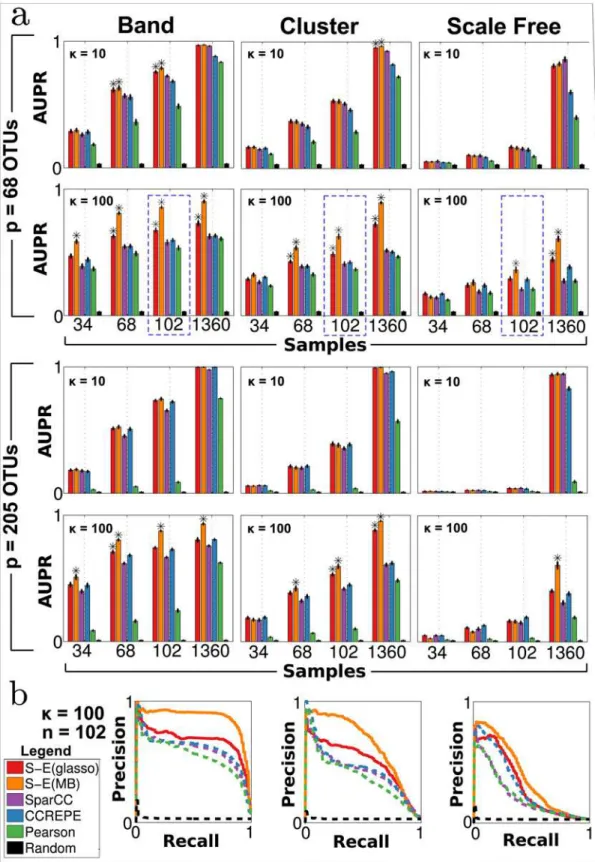
Recovery of microbial networks. To quantify each method’s ability to recover the true underlying association network, we evaluated performance in terms of precision-recall (P-R) curves and area under P-R curves (AUPR). For each method, we ranked edge predictions ac-cording to confidence. For SparCC, CCREPE and Pearson correlation, edge predictions were ranked according to p-value. SPIEC-EASI edge predictions were ranked according to edge sta-bility, inferred by StARS model selection step at the most stable tuning parameterλStARS.Fig 4

summarizes methods’performance on 960 independent synthetic datasets for a total of 48 con-ditions (4 samples sizes × 2 concon-ditions numbers × 3 network topologies × 2 dimensions).

We observe the following key trends. First, the performance of all methods improves with increasing sample size. Under certain scenarios, even near-perfect recovery (AUPR1) is pos-sible in the large sample limit (n= 1360). Second, all methods show a clear dependence on the network topology. Best performance is achieved for band graphs, followed by cluster and scale-free graphs. These results are consistent with theoretical results [29], which show that the maxi-mum node degreedreduces the probability of correctly inferring network edges for fixed sam-ple size (scale-free networks have highest maximum degree, followed by cluster and then band.) Third, for most scenarios, the SPIEC-EASI methods, particularly S-E(MB), perform as well or significantly better than all control methods. Standard Pearson correlation is outper-formed by all methods that take the compositional nature of the data into account. Forth, in the large sample limit (n= 1360), S-E(MB) is the only method that recovers a significant por-tion of edges under all tested scenarios (particularly scale-free networks). Addipor-tionally, we ob-serve (S10 Fig) that SPIEC-EASI performs well on synthetic data generated by the SparCC benchmark [17,59].

Fig 4. Precision-recall performance on synthetic datasets. a) Red = S-E(glasso), orange = S-E(MB), purple = SparCC, blue = CCREPE,

green = Pearson correlation, black = random. Area under precision-recall (AUPR) vs. number of samplesnfor differentκvalues are depicted. Bars represent

average over 20 synthetic datasets, and error bars represent standard error. Asterisks denote conditions under which SPIEC-EASI methods had significantly higher AUPR relative to all other control methods (P<_{0.05 for all one-sided T tests).b) Representative precision-recall curves for}p= 68,n= 102,κ= 100;

solid and dashed lines denote SPIEC-EASI and control methods, respectively.

Overall, these results suggest that S-E methods outperform current state-of-the-art methods in terms of network recovery under most tested scenarios, with S-E(MB) showing superior per-formance over S-E(glasso).

Recovery of global network properties. Accurate recovery of global network properties

(e.g., degree distribution, number of connected components, shortest path lengths) from taxa abundance data would help define the underlying topology of the ecological network (e.g., clus-ter versus scale-free) [15,58]. At this point, little is known about the underlying topology of mi-crobial ecological networks, but, as elaborated in the Discussion, such information could be incorporated as a constraint into SPIEC-EASI’s inference methods, thereby further improving prediction. Thus, we tested how well SPIEC-EASI and other methods recover global network properties from the synthetic datasets and evaluate whether these methods might be able to provide insight into global network architecture, perhaps even in the underdetermined regime, where the prediction of individual edges is less accurate. To control for the disparate means by which individual methods ranked edge confidences (e.g., stability for the SPIEC-EASI methods, estimation of p-values for SparCC, Pearson and CCREPE), for each synthetic dataset and method, final networks were generated by selecting the top 205 predicted edges and comparing to the true synthetic network topologies forp= 205 OTUs.

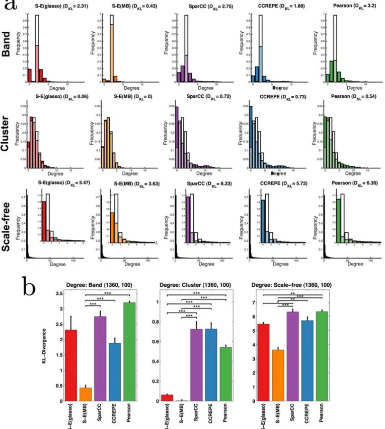
We first consider (node) degree distributions, where node degree is defined as the number of edges each node has. InFig 5, we show the empirical degree distribution and the underlying ground truth for all methods and networks types,n= 1360 andκ= 100. Scale-free networks are characterized by exponential degree distributions, in which few nodes (e.g., hubs and, in our context, potential keystone taxa) have very high degree (e.g., interact with other taxa), while most nodes/taxa have few interactions. In contrast, nodes in cluster networks have rela-tively even degree, which depends on cluster size. In the ecological context, cluster networks would be consistent with niche communities that share few interactions with microbiota out-side of one’s niche community; this structure is also reflected in degree distributions. Using Kullback-Leibler (KL) divergence to measure the dissimilarity between methods’predicted de-gree distributions and the true dede-gree distribution we see that S-E(MB) outperforms all other methods in recovering degree distributions (Fig 5). This performance improvement also holds for smaller samples sizes.

Another common topological feature is betweenness centrality, which, similar to degree, be-tweenness centrality can be used to gauge the relative importance of a node (e.g., taxon) to the (ecological) network. Betweenness centrality, as the fraction of shortest paths between all other nodes in the network that contain the given node, highlights central nodes. The distribution of nodes’betweenness centrality provides information about the network architecture (S4 Fig). Specifically, scale-free networks are expected to have a few nodes with very high betweenness centrality that connect most other nodes to each other; in scale-free networks, betweenness centrality can approach unity. For cluster networks, the maximum betweenness centrality is limited by the total number of independent clusters. In band networks, similar to scale-free, all nodes are connected; however, the degree is fixed and so the betweenness centrality distribu-tion is roughly uniform from zero to one. For smaller sample sizesn<1360, no method domi-nates. However, for the largest sample size,n= 1360, S-E(MB) is again significantly better than all other methods for five out of six conditions with the exception of scale-free networksκ= 10, where SparCC recovery is best (S5 Fig).

Fig 5. a) Predicted degree distributions (colored) are overlaid with the true degree distribution (white) forn= 1360 samples,p= 205 OTUs,κ= 100.

Lighter shades correspond to regions of overlap between predicted and true distributions. Dissimilarity between the distributions is measured by KL divergence,DKL. b) Bars represent the averageDKLover three independent sets of synthetic datasets (7 datasets per set); error bars represent standard error. Divergences were compared between S-E and control methods using one-sided T-tests;***,**,*correspond to P<_{0.001, 0.01, and 0.05.}

distance distributions, S-E(MB) performs equivalently or significantly better than all other methods for scale-free networks as well as band graphs across all conditions. For cluster net-works, the other methods generally outperform SPIEC-EASI methods for smaller sample sizes (n<1360). In the large sample limitn= 1360, S-E(MB) has significantly better recovery of geodesic distance distributions relative to all control methods, even for cluster graphs (S7 Fig).

Finally, we analyzed the number and size of connected components in the inferred graphs. While all synthetic band and scale-free synthetic networks form a single connected component containing all nodes, cluster networks have a variable number of connected components. In terms of cluster number recovery, all methods predicted too many connected components. Overall, S-E methods had lower error rates for band and scale-free networks over all sample sizes. For high sample number (n= 1360), S-E(MB) had significantly better recover of cluster size across all network types (S8 Fig), with nearly perfect recovery for cluster graphs (DKL= 0,

S9 Fig).

Inference of the American Gut network

Thus far we have used then1= 304 first-round AGP samples as a means to construct realistic synthetic microbiome data sets with SPIEC-EASI’s data generation module. In this section, we apply SPIEC-EASI inference methods to construct ecological association networks from the AGP data directly. To do this, we first filter out rare OTUs by selecting only the top 205 OTUs (to match the dimensionality of the synthetic data) in the combined AGP dataset (by frequency of presence) before adding a pseudo-count and total-sum normalization. Although there is no independent means to assess the accuracy of these hypothetical networks, we can assess their reproducibility and consistency. For each method, we first infer a single representative network of taxon-taxon interactions from Round 1 AGP abundance data. For SPIEC-EASI, the StARS model selection approach is used to select the final model network. For SparCC, we use a thresholdρt= 0.35 to construct a relevance network from the SparCC-inferred correlation

ma-trix; i.e. an edge between nodesvi,vjis present in the SparCC network ifjρi,jj>ρt[17].

Similar-ly, we use a q-value cut-off of 10−24_{to create an interaction network from CCREPE-corrected}

significance scores of Pearson’s correlation coefficient [9]. For each method, we thus arrive at a reference network that can be considered the hypothetical gold standard. We then use then2= 254 Round 2 AGP samples as an independent test set and learn a new model network from these data alone. We measure consistency between the two network models by computing the Hamming distance between the reference and new network models, i.e., the difference between the upper triangular part of the two adjacency matrices. For the present data, the Hamming distance can vary betweenp(p−1)/2 = 20910 (no edges in common) and a minimum of 0 for

identical networks. Confidence intervals for Hamming distances can be obtained by combining Round 1 and 2 samples into a unified dataset, repeatedly subsampling these data into two dis-joint groups of sizen1andn2, and repeating the entire inference procedure.

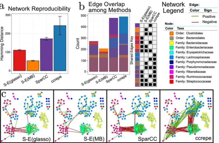
Fig 6ashows network reproducibility for SPIEC-EASI methods, SparCC, and CCREPE. The S-E(MB) has smallest the Hamming distance, followed by S-E(glasso), SparCC, and CCREPE. In S-E(MB), the edge disagreement is roughly 50 with very small error bars. At the other ex-treme, CCREPE edge disagreement is 250 edges and highly variable.

These numerical experiments clearly demonstrate that SPIEC-EASI networks are more re-producible than other current methods.

These edges are mostly found within OTUs of the same taxonomic group. This phenomenon, termed assortativity, has also been observed in other microbial network studies [11]. Assorta-tivity is one of the most salient features of the AGP-derived networks, and, for all networks, the assortativity coefficients for each network are close to unity (e.g., maximum assortativity,S11 Fig). The SparCC network comprises about twice as many edges as the SPIEC-EASI networks. SparCC infers 147 distinct edges; these additional edges correspond to negative associations be-tween OTUs of Ruminococcaceae (genusFaecalibacterium) and Enterobacteriacae families (various genera) and a dense web of correlations within Enterobacteriacae OTUs. Similarly, CCREPE identified 152 edges uniquely, with many negative edges between Enterobacteriaceae and Lachnospiraceae (genera:Blautia,Roseburiaand unknown); additionally, CCREPE uniquely predicted positive edges between the Lachnospiraceae and Ruminococcaceae (genus:

Faecalibacterium). Both SPIEC-EASI methods produce relatively sparse networks by compari-son. S-E(glasso) infers a total of 271 total edges (with one unique edge), and S-E(MB) infers 206 edges with 25 unique edges. In scale with edge predictions, both CCREPE and SparCC infer networks with large maximum degree (33 and 30, respectively), while the S-E(MB) and S-E(glasso) networks have a maximum degree of sixteen and eight, respectively (S11 Fig). However, even though CCREPE and SparCC predict a similar number of total edges, the global

Fig 6. a) Network reproducibility for inference methods (see main text for details).Bars represent mean Hamming distance, and errorbars are 95% confidence intervals. b) Visualization of edge overlap between networks inferred with SPIEC-EASI, SparCC, and CCREPE. c) Network visualizations with OTU nodes colored by Family lineage (or Order, when the Family of the OTU is unknown), edges are colored by sign (positive: green, negative: red), and the node diameter proportional to the geometric mean of that OTU’s relative abundance.

network properties are distinct. CCREPE predicts a higher maximum betweenness centrality and a larger number of nodes in the largest connected component (100).

In summary, analysis of the AGP networks suggests that the SPIEC-EASI inference schemes construct more reproducible taxon-taxon interactions than SparCC and CCREPE and infer considerably sparser model networks than the other two methods. These observations may be explained as follows: SparCC and CCREPE aim to recover correlation networks, which contain both direct edges as well as indirect (e.g., spurious) edges (due to correlation alone). SparCC and CCREPE may recover indirect edges less robustly than direct edges, an explanation that would be consistent with the Hamming distance reproducibility analysis. In addition, all meth-ods’resulting networks suggest that the topology of the American Gut association network cannot be attributed to a specific network class. Instead, these networks are a mixture of band, scale-free, and cluster network type, and they exhibit high phylogenetic assortativity within highly connected components.

Discussion

Inferring interactions among different microbial species within a community and understand-ing their influence on the environment is of central importance in ecology and medicine [19, 60]. An ever increasing number of recent amplicon-based sequencing studies have uncovered strong correlations between microbial community composition and environment in diverse and highly relevant domains of life [1,9,10,61–63]. These studies alone underscore the need to understand how the microbial communities adapt, develop, and interact with the environ-ment [5]. Elucidation of species interactions in microbial communities across different envi-ronments remains, however, a formidable challenge. Foremost, available high-throughput experimental data are compositional in nature, overdispersed, and usually underdetermined with respect to statistical inference. In addition, for most microbes few to no ecological interac-tions are known, thus the ecological interaction network must be constructedde novo, in the absence of guiding assumptions and a set of“gold standard”interactions for validation.

To overcome both challenges, we present SPIEC-EASI (SparseInversE Covariance Estima-tion forEcologicalAssociationInference), a computational framework that includes statistical methods for the inference of microbial ecological interactions from 16S rRNA gene sequencing datasets and a sophisticated synthetic microbiome data generator with controllable underlying species interaction topology. SPIEC-EASI’s inference engine includes two well-known graphi-cal model estimators, neighborhood selection [20] and sparse inverse covariance selection [22, 23,46] that are extended by compositionally robust data transformations for application to the specific context of microbial abundance data.

The synthetic data pipeline was used to generate realistic-looking gut microbiome datasets for a controlled benchmark of SPIEC-EASI’s inference performance relative to two state-of-the-art methods, SparCC [17] and CCREPE [9]. We showed that neighborhood selection (S-E (MB)) outperforms SparCC and CCREPE in terms of recovery of taxon-taxon interactions and global network topology features under almost all tested benchmark scenarios, while covari-ance selection (S-E(glasso)) performs competitively with and sometimes better than SparCC and CCREPE.

network. Our simulation study provides the community with rough guidelines for requisite sample sizes, given state-of-the-art network inference and basic assumptions about the under-lying network. This is of obvious importance to experimental design and the estimation of sta-tistical power. Here, we used the synthetic data pipeline to generate datasets characteristic of the gut microbiome. However, the SPIEC-EASI data generator is generic and therefore enables researchers to generate synthetic datasets that resemble microbiome samples in terms of taxa dispersion and marginal distributions from their field of research, such as soil or sea water eco-systems [1].

Our application study on real American Gut Project (AGP) data revealed that inference with SPIEC-EASI produced more consistent and sparser interaction networks than SparCC and CCREPE. In addition, our AGP network analysis revealed several biologically relevant ob-servations. Specifically, we observed that OTUs were more likely to interact with phylogeneti-cally related OTUs (Fig 6candS11 Fig). In addition, our gut microbial interaction networks appear to be a composite of network types, as we find evidence for scale-free, band-like, and cluster subnetworks.

An important advantage of neighborhood and covariance selection as underlying inference frameworks is their ability to include prior knowledge about the underlying data or network structure from independent scientific studies in a principled manner. For example, in the neighborhood selection scheme, the standard LASSO approach can be augmented by a group penalty [64] that takes into accounta prioriknown group structure. The assortativity observed in our gut microbial interaction networks suggests that such a grouping of OTUs based on phy-logenetic relationship might improve inference. Moreover, if verified species interactions are available for a certain microbial contexts, this knowledge can be included in covariance and neighborhood selection by relaxing the penalty term on these interactions. This strategy has al-ready been fruitfully applied to inference of similarly high-dimensional transcriptional regula-tory networks [65]. Finally, in agreement with theoretical and empirical work in high-dimensional statistics, our synthetic benchmark results confirmed that networks with scale-free structures elude accurate inference even if the underlying network is globally sparse. Re-cent modified neighborhood [30] and covariance selection [31] schemes improve recovery of scale-free networks and can be conveniently included into SPIEC-EASI.

Finally, although the main focus of this work is inference of microbial interaction networks, estimation of the regularized inverse covariance matrix with S-E(glasso) will be key to address-ing several other important questions arisaddress-ing from microbiome studies. For example, statistical methods to infer which taxa are responsive to design factors in 16S gene amplicon studies is an active area of research. Most methods test each taxon independently one-at-a-time (see [56] and references therein) even though taxa are actually highly correlated and thought to ecolog-ically interact. Inference of taxa responses from 16S rRNA gene sequencing datasets could be improved by modeling this correlation structure through incorporation of the inverse covari-ance matrix into the statistical model [66].

Other, more complex questions are motivated by a desire to understand why and how eco-systems evolve with time. In the dynamic modeling setting, association networks have already been successfully used as an underlying structure to fit a differential-equation-based model of gut microbiome development in mice [14]. Thus, association networks provide the underlying topology for dynamic models, which can be used to develop hypotheses about how the ecosys-tems might respond to specific perturbations [5].

methods provide a flexible and principled mathematical framework to incorporate additional information about microbial ecological association networks as it becomes available, thereby improving prediction. We anticipate that SPIEC-EASI network inference will serve as a back-bone for more sophisticated modeling endeavors, engendering new hypotheses and predictions of relevance to environmental ecology and medicine.

Supporting Information

S1 Text. Comparative marginal fits to American Gut Project count data.A discussion of the

methods used to simulate biologically-plausible correlated count data, and some results com-paring different generative distributions.

(PDF)

S1 Table. Method comparison.Table to compare some of the features of SPIEC-EASI,

SparCC, CCREPE and Pearson’s correlation coefficient. (PDF)

S1 Fig. Relationship between target and empirical correlation after NorTA transformation.

The recovery of empirical Pearson correlations generated from the NORTA process, using zero-inflated Negative Binomial as a model (x-axis) verses the input multivariate Normal em-pirical correlations (upper panels) or inverse correlations (lower panels) on untransformed counts (a) or log-transformed counts (b). Simulated data are withp= 205 OTUs,n= 20,000 samples with 10 replicates on each plot.

(PDF)

S2 Fig. Heatmaps of AGP and synthetic data.Visual comparison of American Gut Project

data with synthetically generated datasets. Heatmaps show log10(counts). For all network types (band, graph, scale-free), synthetic datasets are consistent with real datasets in terms of number of OTUs, number of samples, and OTU count abundances across samples.

(PDF)

S3 Fig. Effect of Condition Number on Correlations Distribution.The condition of a

Preci-sion matrix is the ratio of the largest to smallest eigenvalue/singular value. The relationship be-tween condition number and correlation distribution for the synthetic networks; increasing condition number corresponds to increasing the strength of correlations in the network. (PDF)

S4 Fig. Betweenness Centrality for Synthetic Networks.Examples of betweenness centrality

distributions for each network type (in white) overlayed with the distribution predicted by S-E (MB) (in orange) forκ= 100,n= 1360 samples,p= 205 OTUs.

(PDF)

S5 Fig. Recovery Performance of Betweenness Centrality.Performance results for

between-ness centrality (red = S-E(glasso) orange = S-E(MB), purple = SparCC, blue = CCREPE, green = Pearson). Bars represent the average KL-divergence over three independent sets of syn-thetic datasets (7 datasets per set); error bars represent standard error. Asterisks indicate that an S-E method had siginificantly better recovery of the true betweenness centrality distribu-tions (p<0.05 for one-sided T tests in comparison to each control method).

S6 Fig. Geodesic Distance for Synthetic Networks.Examples of geodesic distance distribu-tions for each network type (in white) overlaid with the distribution predicted by S-E(MB) (in orange) forκ= 100,n= 1360 samples,p= 205 OTUs

(PDF)

S7 Fig. Recovery Performance of Geodesic Distance.Performance results for geodesic

dis-tance distributions (red = S-E(glasso), orange = S-E(MB), purple = SparCC, blue = CCREPE, green = Pearson). Bars represent the average KL-divergence over three independent sets of syn-thetic datasets (7 datasets per set); error bars represent standard error. Asterisks indicate that an S-E method had significantly better recovery of the true geodesic distance distributions (p<0.05 for one-sided T tests in comparison to each control method).

(PDF)

S8 Fig. Cluster Sizes for Synthetic Networks.Examples of cluster size distributions for each network type (in white) overlayed with the distribution predicted by S-E(MB) (in orange), for κ= 100,n= 1360 samples,p= 205 OTUs.

(PDF)

S9 Fig. Recovery Performance of Cluster Sizes.Performance results for cluster size distribu-tions (red = S-E(glasso), orange = S-E(MB), purple = SparCC, blue = CCREPE,

green = Pearson). Bars represent the average KL-divergence over three independent sets of syn-thetic datasets (7 datasets per set); error bars represent standard error. Asterisks indicate that an S-E method had significantly better recovery of the true cluster size distributions (P<0.05 for one-sided T tests in comparison to each control method).

(PDF)

S10 Fig. Synthetic test case from SparCC.Using the example data provided by the SparCC

package, we inferred networks from SparCC (threshold correlation at ±.35), S-E(MB) and CCREPE (thresholding q-value at 5₁₀−19_{). In this setting, SparCC and SPIEC-EASI correctly}

recover four true edges, including the association sign. (PDF)

S11 Fig. Assortativity coefficients in inferred American Gut networks.Network assortativity coefficients at the Phyla and Family level for each of the four inference methods. Assortativity is a measure of the tendency for nodes to be connected with nodes of the same taxonomic class. (PDF)

Acknowledgments

We would like to thank Eric Alm and Jonathan Friedman for helpful discussions.

Author Contributions

Conceived and designed the experiments: ZDK CLM ERM RAB. Performed the experiments: ZDK CLM ERM. Analyzed the data: ZKD CLM ERM RAB. Contributed reagents/materials/ analysis tools: ZKD CLM ERM. Wrote the paper: ZKD CLM ERM DRL MJB RAB.

References

2. Turnbaugh PJ, Ley RE, Hamady M, Fraser-Liggett C, Knight R, et al. (2007) The human microbiome project: exploring the microbial part of ourselves in a changing world. Nature 449: 804. doi:10.1038/ nature06244PMID:17943116

3. AmGut. The american gut project.http://humanfoodproject.com/americangut/. Accessed: 2014-01-30. 4. Bunge J, Willis A, Walsh F (2014) Estimating the number of species in microbial diversity studies.

Annu-al Review of Statistics and Its Application 1: 427–445. doi:10.1146/annurev-statistics-022513-115654 5. Foster JA, Krone SM, Forney LJ (2008) Application of ecological network theory to the human

micro-biome. Interdisciplinary perspectives on infectious diseases 2008: 839501. doi:10.1155/2008/839501 PMID:19259330

6. Arumugam M, Raes J, Pelletier E, Le Paslier D, Yamada T, et al. (2011) Enterotypes of the human gut microbiome. Nature 473: 174–180. doi:10.1038/nature09944PMID:21508958

7. Koren O, Knights D, Gonzalez A, Waldron L, Segata N, et al. (2013) A guide to enterotypes across the human body: meta-analysis of microbial community structures in human microbiome datasets. PLoS computational biology 9: e1002863. doi:10.1371/journal.pcbi.1002863PMID:23326225

8. Chen J, Li H (2013) Variable selection for sparse dirichlet-multinomial regression with an application to microbiome data analysis. The Annals of Applied Statistics 7: 418–442. doi:10.1214/12-AOAS592 9. Gevers D, Kugathasan S, Denson LA, Vázquez-Baeza Y, Van Treuren W, et al. (2014) The

treatment-naive microbiome in new-onset crohn’s disease. Cell Host—Microbe 15: 382–392. doi:10.1016/j. chom.2014.02.005PMID:24629344

10. Lee SC, Tang MS, Lim YAL, Choy SH, Kurtz ZD, et al. (2014) Helminth colonization is associated with increased diversity of the gut microbiota. PLoS Negl Trop Dis 8: e2880. doi:10.1371/journal.pntd. 0002880PMID:24851867

11. Faust K, Sathirapongsasuti JF, Izard J, Segata N, Gevers D, et al. (2012) Microbial Co-occurence Rela-tionships in the Human Microbiome. PLoS Computational Biology 8: e1002606. doi:10.1371/journal. pcbi.1002606PMID:22807668

12. Fuhrman JA, Steele JA (2008) Community structure of marine bacterioplankton: Patterns, networks, and relationships to function. In: Aquatic Microbial Ecology. volume 53, pp. 69–81. doi:10.3354/ ame01222

13. Barberán A, Bates ST, Casamayor EO, Fierer N (2012) Using network analysis to explore cooccur-rence patterns in soil microbial communities. The ISME journal 6: 343–51. doi:10.1038/ismej.2011. 119PMID:21900968

14. Marino S, Baxter NT, Huffnagle GB, Petrosino JF, Schloss PD (2014) Mathematical modeling of prima-ry succession of murine intestinal microbiota. Proceedings of the National Academy of Sciences of the United States of America 111: 439–44. doi:10.1073/pnas.1311322111PMID:24367073

15. Deng Y, Jiang YH, Yang Y, He Z, Luo F, et al. (2012) Molecular ecological network analyses. BMC Bio-informatics 13: 113. doi:10.1186/1471-2105-13-113PMID:22646978

16. Steele Ja, Countway PD, Xia L, Vigil PD, Beman JM, et al. (2011) Marine bacterial, archaeal and protis-tan association networks reveal ecological linkages. The ISME journal 5: 1414–25. doi:10.1038/ismej. 2011.24PMID:21430787

17. Friedman J, Alm EJ (2012) Inferring correlation networks from genomic survey data. PLoS computa-tional biology 8: e1002687. doi:10.1371/journal.pcbi.1002687PMID:23028285

18. Aitchison J (1981) A new approach to null correlations of proportions. Mathematical Geology 13: 175–

189. doi:10.1007/BF01031393

19. Faust K, Raes J (2012) Microbial interactions: from networks to models. Nat Rev Micro 10: 538–550. doi:10.1038/nrmicro2832

20. Meinshausen N, Bühlmann P (2006) High Dimensional Graphs and Variable Selection with the Lasso. The Annals of Statistics 34: 1436–1462. doi:10.1214/009053606000000281

21. Bonneau R, Reiss D, Shannon P, Facciotti M, Hood L, et al. (2006) The inferelator: an algorithm for learning parsimonious regulatory networks from systems-biology data sets de novo. Genome Biology 7: R36. doi:10.1186/gb-2006-7-5-r36PMID:16686963

22. Friedman J, Hastie T, Tibshirani R (2008) Sparse inverse covariance estimation with the graphical lasso. Biostatistics (Oxford, England) 9: 432–441. doi:10.1093/biostatistics/kxm045

23. Banerjee O, El Ghaoui L, d’Aspremont A (2008) Model selection through sparse maximum likelihood estimation for multivariate gaussian or binary data. The Journal of Machine. . .9: 485–516. 24. Wille A, Zimmermann P, Vranová E, Fürholz A, Laule O, et al. (2004) Sparse graphical Gaussian