www.adv-radio-sci.net/11/47/2013/ doi:10.5194/ars-11-47-2013
© Author(s) 2013. CC Attribution 3.0 License.
Radio Science
A fully probe corrected near-field far-field transformation technique
employing plane-wave synthesis
R. A. M. Mauermayer and T. F. Eibert
Lehrstuhl f¨ur Hochfrequenztechnik, Technische Universit¨at M¨unchen, 80290 Munich, Germany Correspondence to:R. A. M. Mauermayer ([email protected])
Abstract. The far-field behavior of an antenna under test (AUT) can be obtained by exciting the AUT with a plane wave. In a measurement, it is sufficient if the plane wave is artificially generated in the vicinity of the AUT. This can be achieved by using a virtual antenna array formed by a probe antenna which is sequentially sampling the radiating near-field of the AUT at different positions. For this purpose, an optimal filter for the virtual antenna array is computed in a preprocessing step. Applying this filter to the near-field mea-surements, the far-field of the AUT is obtained according to the propagation direction and polarization of the synthesized plane wave. This means that the near-field far-field transfor-mation (NFFFT) is achieved simply by filtering the near-field measurement data. Taking the radiation characteristic of the probe antenna into account during the synthesis process, its influence on the NFFFT is compensated.
The principle of the plane-wave synthesis and its applica-tion to the NFFFT is presented in detail in this paper. Further-more, the method is verified by performing transformations of simulated near-field measurement data and of near-field data measured in an anechoic chamber.
1 Introduction
Today’s wireless communication, radar or direction finding systems make use of electrically large antennas like parabolic reflectors or antenna arrays to generate far-field radiation characteristics suitable for the particular application. After fabrication the far-field of the antenna under test has to be examined by measurements to verify that it meets the re-quirements on phase and magnitude. Due to the large size of the antenna relative to wavelength, an accurate measure-ment under far-field conditions inside an anechoic chamber can hardly be accomplished, simply because of the enormous measurement distance required. Thus, performing
measure-ments in a reduced distance in the radiating near-field region of the AUT and subsequently applying a near-field far-field (NFFF) transformation is an attractive alternative.
The radiated fields of the AUT and the probe are usu-ally represented by a truncated series of orthogonal spheri-cal, cylindrical or planar field modes to formulate a transmis-sion equation describing the coupling between both antennas (Hansen, 1988). Solving this equation for the modal coeffi-cients the far-field can be computed by evaluating the field modes for the radial distance going to infinity.
For the plane-wave synthesis approach (Hansen, 1988; Ya-maguchi et al., 2009; Bennett and Schoessow, 1978), there is no explicit transmission equation needed. The probe which is sampling the near-field successively at different locations is considered to form a virtual array of probe antennas on a measurement surface. This array is then used to synthesize a plane wave in the vicinity of the AUT through a weighted superposition of the fields radiated by the elements of the virtual probe antenna array. The appropriate weights form a filter which is gained from the solution of an inverse problem. The proposed method allows shifting most of the compu-tational expense of the NFFF transformation and probe cor-rection to a preprocessing step whose result is a set of filters containing the weighting factors for the probe signals. These filters are used to compute the far-field directly from the ac-quired measurement data in a near-field far-field transforma-tion step.
2 The probe corrected plane-wave synthesis
2.1 Principle
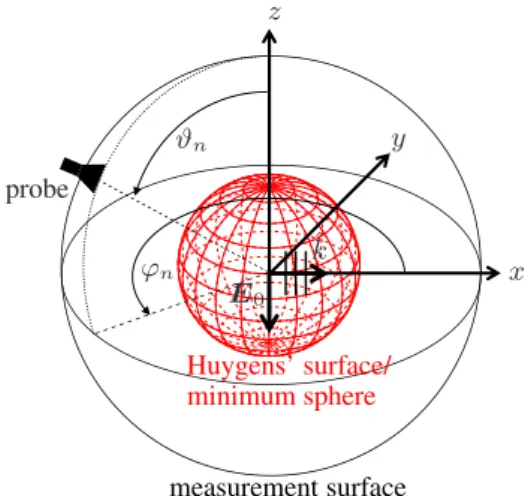
The principle of the synthesis of plane waves by a virtual ar-ray of probes which are positioned at different locations in the near-field of the AUT is visualized in Fig. 1. The probes are excited according to the filter vectorw
ˆ
k,E0
, which consists ofN complex coefficients, one for each probe posi-tion and polarizaposi-tion orientaposi-tion. The objective is to generate the field of the plane wave
Epl(r)=E0e−j kkˆ·r (1)
Hpl(r)= 1
Z0
ˆ
k×Epl(r) (2)
in the vicinity of the AUT by superimposing the probe fields. The propagation direction of the plane wave is described by the unit vectorkˆ and its polarization is given by the electric field vectorE0.Z0describes the free space wave impedance. The virtual array is equivalent to a probe antenna with ideal polarization purity positioned in the far-field of the AUT in direction − ˆk and exciting the AUT with a quasi plane-wave field with the same polarization as the synthe-sized plane wave. The power wavebFF1
ˆ
k,E0
at the feed point of the AUT in Fig. 1 is proportional to this far-field measurement.
For the wave field synthesis process inside a volume, the AUT is enclosed by a Huygens’ surface. A filter must be found that enables the synthesis of the tangential field com-ponents of the desired plane wave on the surface. The unique-ness theorem (Harrington, 2001) guarantees that if the super-imposed tangential field components of the virtual probe ar-ray correspond to those of the plane wave, the plane-wave field is also present inside the source free test volume.
The probe antenna is modeled by its equivalent electric Jn r′and magneticMn r′surface currents located at the
n-th probe sampling position. Its characteristic electromag-netic field is computed from the surface integrals
En(r)=
Z Z
A h
¯
GEJ r,r′·Jn r′
+ ¯GEM r,r′·Mn r′idA′ (3)
Hn(r)=
Z Z
A h
¯
GHJ r,r′·Jn r′
+ ¯GHM r,r′·Mn r′idA′, (4)
whereG¯E/HJ /M r,r′are the dyadic Greens’ functions for free space. The tangential components of the probe field are sam-pled at discrete locationsri (i=1, . . . , I )on the Huygens’ surface. In order to avoid the excitation of resonance modes
bFF 1(ˆk,E0)
E0 ˆ k virtual probe filterw ˆ k,E0 a2 w1 ˆ k,E0 w2 ˆ k,E0 w3 ˆ k,E0 wN ˆ k,E0 array AUT
Fig. 1.The principle of plane-wave synthesis by a virtual array of probes positioned in the near-field region of the AUT. The AUT
consists of six antenna elements. The power wavebFF1
ˆ k,E0
is measured at the feed point of one antenna element.
inside the test volume, the combined field vector (Hansen, 1988)
Fn(ri)=En(ri)|tan−Z0n×Hn(ri) (5)
is used, withnbeing the normal vector of the Huygens’ sur-face. The constraint that the tangential components of the su-perimposed probe fields have to be equal to that of the plane wave leads to the equation system
F1(r1) . . .FN(r1)
F1(r2) . . .FN(r2) ..
. . .. ...
F1(rI) . . . FN(rI)
| {z }
F w1 ˆ
k,E0
.. . wN ˆ
k,E0
| {z }
wk,ˆE0
=
Fpl(r1) .. .
Fpl(rI)
| {z }
Fpl
(6) of the inverse problem withFpl(ri)being the combined field vector evaluated for the plane wave. As there are usually more sampling pointsI on the Huygens’ surface than probe positionsN, the equation system is over-determined. There-fore, it is solved for the filter coefficients in a least mean square error sense in form of
w
ˆ
k,E0
=F+Fpl (7)
using the pseudoinverseF+of matrixFin Eq. (6). This so-lution also minimizes the norm of the filter vector and the power radiated by the virtual probe antenna array, respec-tively.
For this synthesis problem, the field components of the probe are directly sampled in the flat area instead of sam-pling the tangential field components on a Huygens’ surface. However the kind of inverse problem remains the same and it is solved in the same way as described above.
2.2 Measurement setups and sampling conditions
The measurement setup has to be defined for the synthesis process. There are two setups for the investigation of the plane-wave synthesis inside a volume and on a planar area.
For the synthesis in a volume the spherical measurement setup depicted in Fig. 2a is considered. The probe is posi-tioned on a spherical measurement surface with radius 1 m. At each position of the regular sampling grid inϑandϕ di-rection the probe is oriented with vertical and horizontal po-larization. The probe sampling rate, which depends on wave-lengthλand the radiusρof the minimum sphere, is derived from the sampling condition (Yaghjian, 1986)
1ϑ=1ϕ≤ λ
2(ρ+λ) (8)
for conventional NFFFT using spherical multipoles. The Huygens’ surface is formed by the minimum sphere which encloses the AUT and has a radius ofρ=0.5 m.
For the synthesis of a plane wave on a planar area the setup shown in Fig. 2b is used. The intention here is to generate a field distribution on the disc with radius 0.5 m that is more similar to a plane wave than the field of the probe antenna itself. The probe is positioned on a measurement circle in thexy plane with radius 1.98 m. Again the probe sampling interval inϕdirection is chosen following Eq. (8).
The sampling point distance of the probe fields on the Huygens’ surface and on the disc is chosen to be smaller than
λ/2 according to the Nyquist-Shannon sampling theorem.
2.3 Filter coefficients
For the spherical measurement, an open ended rectangular waveguide probe operating at 2 GHz is used. It is positioned on the measurement surface in 5◦steps inϑandϕdirection. The tangential field components on the Huygens’ surface are also sampled on a regular grid inϑandϕdirection in 6◦ in-tervals. For all probe positions the probe fields are computed on the Huygens’ surface by Eq. (3) and Eq. (4). The sampled tangential components result in the columns of matrixF in Eq. (6). The plane wave that is to be synthesized is propa-gating in positivex direction and is vertically polarized as it is given in Fig. 2a. The necessary filter coefficients for the optimal synthesis of the plane wave are gained from the so-lution of the equation system according to Eq. (7). In Fig. 3 the resulting normalized magnitude of the filter coefficients is shown. As the probe is vertically and horizontally oriented there is one filter coefficient for each of the probe polariza-tion states. It can be clearly seen that most of the power is
probe
measurement surface
Huygens’ surface/ minimum sphere
z
y
x
ϑn
ϕn
ˆ
k
E0
(a) Spherical measurement setup. A plane wave is synthesized inside the minimum sphere en-closing the AUT with propagation directionˆk=
exand vertical polarizationE0=−ez
probe
measurement circle disc
ϕn y
x
E0
ˆ
k
(b) Measurement setup for plane-wave synthesis on a disc. The probe is rotated on the measure-ment circle.
Fig. 2.Measurement setups for plane-wave synthesis inside a
vol-ume(a)and on a disc(b).
radiated by the vertically polarized probes which are radiat-ing in propagation direction of the plane wave whereas the horizontally oriented probes are excited with less power be-cause their radiated fields have a dominant horizontal electric field component and fit less to the vertically polarized plane wave.
ϕin degree
ϑ
in
d
eg
re
e
0 30 60 90 120 150 180 210 240 270 300 330 2.5
27.5 52.5 77.5 102.5 127.5 152.5 177.5
(a) vertical polarization
ϕin degree
ϑ
in
d
eg
re
e
m
ag
n
it
u
d
e
in
d
B
0 30 60 90 120 150 180 210 240 270 300 330
≤-60 -40 -20 0 2.5
27.5 52.5 77.5 102.5 127.5 152.5 177.5
(b) horizontal polarization
Fig. 3.Normalized magnitude of the filter coefficients for a vertically(a)and a horizontally(b)polarized open ended waveguide probe
synthesizing a vertically polarized plane wave propagating in positivexdirection.
n
o
rm
al
iz
ed
m
ag
n
it
u
d
e
in
d
B
ϕin degree
0 30 60 90 120 150 180 210 240 270 300 330
-30 -25 -20 -15 -10 -5 0
Fig. 4.Normalized magnitude of the filter coefficients for the syn-thesis on a disc.
setup, most of the power is radiated by the elements of the virtual probe antenna array which are already pointing in the propagation direction of the plane wave, i.e. probes on the measurement circle withϕnaround 180◦.
2.4 Wave field synthesis results
The elements of the virtual probe array are excited according to the computed filter coefficients. The most important ac-curacy measure of the synthesis method is the quality of the wave field which is generated. Since the quality of the plane wave determines the accuracy of the following NFFF trans-formation process. Therefore, the deviation of the magnitude and phase of the synthesized wave field from the ideal plane wave is regarded.
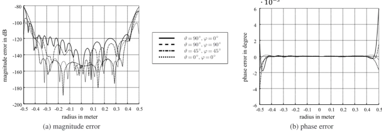
In the case of the spherical setup, the errors are computed on lines which are crossing the minimum sphere in different directions to get an impression of the electrical field distribu-tion inside the volume. The deviadistribu-tions are shown in Fig. 5. The magnitude error of the generated wave field is lower than
−80 dB. The phase error is smaller than 0.006◦. As only thez
component of the synthesized electric field is considered, the polarization purity was checked to be above 80 dB inside the minimum sphere. It is possible to further increase the
qual-ity of the synthesized plane wave by increasing the sampling rate of the probe on the measurement surface.
The errors of the plane wave synthesized on the disc are shown in Fig. 6. The magnitude shows a maximum devia-tion of about−17 dB and the phase of about 2◦. It should be mentioned that the errors increase below and above the con-sidered planar region inzdirection. Nevertheless, as it was intended, the superimposed field on the disc of the virtual array is more similar to a plane wave than the field of only one probe on the measurement circle, which would result in a maximum deviation of−11 dB in magnitude and 140◦in phase.
In general, a closed boundary surface with the appropriate impressed equivalent surface currents is mandatory for the accurate generation of a desired wave field. For the synthe-sis of the plane wave on a disc, this assumption is violated since the virtual probe array only forms kind of a line cur-rent around the disc. Therefore an accurate synthesis of the desired wave field cannot be achieved.
3 NFFFT based on plane-wave synthesis
To find a relation between the near-field measurements and the AUT far-field, the signal flow in Fig. 1 is inverted so that the transposed system shown in Fig. 7 is obtained. This can be done due to the assumption of the reciprocity prop-erty of the whole system. The far-field of the AUT in direc-tion− ˆk, which is now proportional to the power wave signal
b2F F
ˆ
k,E0
, is computed by
b2F F
ˆ
k,E0
=
N X
n=1
wn
ˆ
k,E0
b2N F,n (9)
applying the filter coefficientswn
ˆ
k,E0
to the power wave signalsbNF2,n received by the probe at positionnin the AUT near-field. From Eq. (9) it is obvious that the NFFF transfor-mation employing plane-wave synthesis is just a filtering of the near-field data.
-0.5 -0.4 -0.3 -0.2 -0.1 0 0.1 0.2 0.3 0.4 0.5 -200 -180 -160 -140 -120 -100 -80 m ag n it u d e erro r in d B
radius in meter
(a) magnitude error
ϑ= 90◦,ϕ= 0◦
ϑ= 90◦,ϕ= 90◦
ϑ= 45◦,ϕ= 45◦
ϑ= 0◦,ϕ= 0◦
radius in meter
-0.5 -0.4 -0.3 -0.2 -0.1 0 0.1 0.2 0.3 0.4 0.5 -6 -4 -2 0 2 4 6 p h as e erro r in d eg re e
∙ 0−
(b) phase error
Fig. 5.Magnitude and phase error of the synthesized plane wave evaluated on several lines crossing the minimum sphere in different directions.
xin m
y in m m ag n it u d e er ro r in d B
1.6 1.8 2 2.2 2.4 ≤-60
-55 -50 -45 -40 -35 -30 -25 -20 -0.5 -0.4 -0.3 -0.2 -0.1 0 0.1 0.2 0.3 0.4 0.5
(a) magnitude error
xin m
y in m p h as e er ro r in d eg re e
1.6 1.8 2 2.2 2.4
-2 -1.5 -1 -0.5 0 0.5 1 1.5 2 -0.5 -0.4 -0.3 -0.2 -0.1 0 0.1 0.2 0.3 0.4 0.5
(b) phase error
Fig. 6.Magnitude and phase error of the synthesized plane wave on a disc.
a1
filterwk,ˆE0
bF F2
ˆ k,E0 w1 ˆ k,E0
w2
ˆ k,E0
w3 ˆ k,E0 wN ˆ k,E0
bNF2,1
bNF 2,N
AUT
Fig. 7.Considered system for the NFFFT employing plane-wave synthesis.
rotated inϕ direction by a cyclic rotation of the filter coef-ficients taking advantage of the rotational symmetry of the probe sampling points on the measurement and of the Huy-gens’ surface. This allows to determine a horizontal cut of the AUT far-field pattern (E-plane) without having to solve the inverse problem of Eq. (6) for eachϕangle of plane wave incidence again.
4 Application of the NFFFT based on plane-wave
synthesis
4.1 Simulated and measured near-field data
52 R. A. M. Mauermayer and T. F. Eibert: A fully probe corrected NFFFT technique employing plane-wave synthesis
✲ ✶✺ ✵ ✲ ✶✵ ✵ ✲✺ ✵ ✵ ✺ ✵ ✶ ✵✵ ✶✺✵ ✵
✺✵
✶ ✵✵
✶✺ ✵
in degree
in
d
eg
re
e
✲6✵ ✲✺✵ ✲4✵ ✲3✵ 2✁ ✂✁ ✵
m
ag
n
it
u
d
e
in
d
Fig. 8.Normalized magnitude of the probe signal for copolar orien-tation of the waveguide probe.
The NFFFT based on the wave field synthesis on a disc is verified applying it to simulated near-field data acquired by the horn antenna probe in the near-field of a patch antenna. This simulation scenario is also built up in an anechoic cham-ber, shown in Fig. 10, and real measurements are recorded. Since the AUT represents one element of a circular antenna array it is mounted to a construction made from Rohacell so that the patch antenna pattern is not disturbed by the mount-ing. The normalized, simulated and measured probe signals are plotted in Fig. 9.
Both AUT antennas are positioned in 0.3 m distance to the rotational axis as they represent the antenna element of a cir-cular antenna array which is sketched in Fig. 1.
The simulated and real measurement setups, including the probe and sampling rates, are the same as for the synthesis processes, so the computed filters can be directly applied to the simulated and measured near-field data for NFFF trans-formation.
4.2 NFFF transformation results
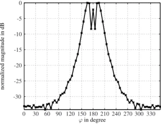
For the spherical NFFF transformation the filter of Fig. 3 is directly applied to the acquired near-field data of Fig. 8. Eval-uating Eq. (9) for the cyclically rotated versions of the filter coefficients leads to the horizontal cut (H-plane) of the far-field pattern. The transformation result compared to the ref-erence solution computed by FEKO is given in Fig. 11. As it is to be expected from the high quality of the synthesized plane wave in the vicinity of the AUT there is no difference recognizable between reference and NFFFT results. Regard-ing the errors of the transformation in Fig. 12, it can be seen that the error of the normalized far-field magnitude is below
−80 dB and the phase error is in the range of some thou-sandths of one degree. So the transformation errors are in the range of the magnitude and phase errors of the synthesized plane wave.
Already from the quality of the synthesized plane-wave field on the disc it can be derived that the transformation results of the near-field data acquired on the measurement circle cannot reach the accuracy as the one of the complete spherical measurement. Figure 13 shows the results of the
✲ ✶✺ ✵ ✲ ✶✵ ✵ ✲✺ ✵ ✵ ✺ ✵ ✶ ✵✵ ✶✺✵ ✺✵
✶ ✵✵
✶✺ ✵
✲✵ ✲✺✵ ✲✵ ✲✵ ✁
measurement simulation
-20 dB -10 dB
0 dB
30
210
60
240
90
270 120
300 150
330
180 0 ϕ
Fig. 9.Simulated and measured near-field data acquired on the mea-surement circle.
✲ ✶✺ ✵ ✲ ✶✵ ✵ ✲✺ ✵ ✵ ✺ ✵ ✶ ✵✵ ✶✺✵ ✵
✺✵
✶ ✵✵
✶✺ ✵
✲✵ ✲✺✵ ✲✵ ✲✵ ✁ ✂✁ ✵
positioner
Fig. 10.Measurement setup in an anechoic chamber for the NFFFT based on the plane-wave synthesis on a disc.
NFFF transformation for the simulated and measured near-field data. For the simulated data, the transformation result matches very well to the reference of the patch antenna far-field pattern.
-15 dB -10 dB
-5 dB 0 dB
30
210
60
240
90
270 120
300 150
330
180 0 ϕ
reference
NFFFT
Fig. 11.Magnitude of reference and transformed far-field.
2 4 6 8 2 4 6 8
2 8 6 4 2
2 4 6 8 2 4 6 8
. . . . . .
err
or o
norm
a
i
ed
m
agni
tude
i
n d
pha
se
e
rr
or i
n
de
gr
ee
in degree
Fig. 12.Errors of normalized magnitude and phase of the transfor-mation result for the spherical near-field measurement.
this seems to be that the measurement was done in a facility that is not appropriate for near-field measurements, so that the exact positioning and orientation of AUT and probe an-tennas could not be guaranteed. This means that the probe field on the disc which was assumed for the synthesis might have been different from the probe field during the measure-ment in the anechoic chamber. This also explains the dif-ference between simulated and measured near-field data in Fig. 9.
5 Conclusions
The presented near-field far-field transformation technique based on plane-wave synthesis allows to split the transforma-tion process into two steps. In the first step, the plane wave is synthesized by solving an inverse problem for the filter vector for the virtual probe array, which might be time con-suming. In the second step, the transformation of the near-field data can be performed by a faster filtering procedure.
reference near-field data NFFFT
-20 dB -10 dB
0 dB
30
210
60
240
90
270 120
300 150
330
180 0 ϕ
(a) simulation
-20 dB -10 dB
0 dB
30
210
60
240
90
270 120
300 150
330
180 0 ϕ
(b) measurement
Fig. 13.Results of the NFFF transformation of the simulated and measured near-field data acquired on the measurement circle.
The method was verified by applying it to simulated and real near-field measurement data.
References
Bennett, J. and Schoessow, E.: Antenna near-field/far-field trans-formation using a plane-wave-synthesis technique, Proceed-ings of the Institution of Electrical Engineers, 125, 179–184, doi:10.1049/piee.1978.0048, 1978.
EM Software and Systems: FEKO Suite 6.1, http://www.feko.info, 2011.
Hansen, J. E.: Spherical near-field antenna measurements, IEE Electromagnetic Waves Series 26, Peter Peregrinus Ltd., Lon-don, UK, 1988.
Harrington, R. F.: Time-Harmonic Electromagnetic Fields, Wiley, J., Weinheim, 2001.
Yaghjian, A.: An overview of near-field antenna measurements, IEEE Transactions on Antennas and Propagation, 34, 30–45, doi:10.1109/TAP.1986.1143727, 1986.