Artificial periodic irregularities in the auroral ionosphere
M. T. Rietveld1,2, E. Turunen3, H. Matveinen3, N. P. Goncharov4, P. Pollari5 1 Max-Planck-Institut fu¨r Aeronomie, Postfach 20, D-37191 Katlenburg Lindau 3, Germany ([email protected])
2 also at EISCAT, N-9027 Ramfjordmoen, Norway
3 Sodankyla¨ Geophysical Observatory, FIN-99600 Sodankyla¨, Finland ([email protected])
4 Radiophysical Research Institute (NIRFI), Nizhny Novgorod, 603600 Russia ([email protected]) 5 Department of Physical Sciences, University of Oulu, FIN-90570 Oulu, Finland ([email protected])
Received: 15 March 1996/Revised: 2 July 1996/Accepted: 3 July 1996
Abstract. Artificial periodic irregularities (API) are pro-duced in the ionospheric plasma by a powerful standing electromagnetic wave reflected off the F region. The re-sulting electron-density irregularities can scatter other high-frequency waves if the Bragg scattering condition is met. Such measurements have been performed at mid-latitudes for two decades and have been developed into a useful ionospheric diagnostic technique. We report here the first measurements from a high-latitude station, using the EISCAT heating facility near Tromsø, Norway. Both F-region and lower-altitude ionospheric echoes have been obtained, but the bulk of the data has been in the E and D regions with echoes extending down to 52-km altitude. Examples of API are shown, mainly from the D region, together with simultaneous VHF incoherent-scatter-radar (ISR) data. Vertical velocities derived from the rate of phase change during the irregularity decay are shown and compared with velocities derived from the ISR. Some of the API-derived velocities in the 75—115-km height range appear consistent with vertical neutral winds as shown by their magnitudes and by evidence of gravity waves, while other data in the 50—70-km range show an unrealistically large bias. For a comparison with ISR data it has proved difficult to get good quality data sets overlapping in height and time. The initial comparisons show some agreement, but discrepancies of several metres per second do not yet allow us to conclude that the two techniques are measur-ing the same quantity. The irregularity decay time-con-stants between about 53 and 70 km are compared with the results of an advanced ion-chemistry model, and height profiles of recorded signal power are compared with model estimates in the same altitude range. The calculated amplitude shows good agreement with the data in that the maximum occurs at about the same height as that of the measured amplitude. The calculated time-constant agrees very well with the data below 60 km but is larger above 60 km by a factor of up to 2 at 64 km. The comparisons
Correspondence to: M. T. Rietveld
with the model are considered to be a good basis for more refined comparisons.
1 Introduction
A high-frequency (HF) radio wave which reflects off the F-region plasma sets up a standing-wave pattern which may extend to quite low altitudes. If the field strength of the wave is strong enough, it may change the electron density at the interference maxima by one of several differ-ent mechanisms depending on the altitude. Above about 130 km the ponderomotive force of the HF wave, which is proportional to the gradient of the time-averaged square magnitude of the electric field, can redistribute the elec-tron density directly. Near the point of reflection of an O-mode wave, Langmuir waves are produced whose pon-deromotive force can drive the artificial periodic irregular-ities (API) because the ponderomotive force of the Langmuir waves is much stronger than that of the HF waves.
Below about 120 km the Ohmic heating of electrons results in electron-density changes because of the depend-ence of the ambipolar diffusion coefficient and the recom-bination rate on the electron temperature,¹
e, and below
about 70 km because the electron attachment rate to molecules depends on¹
e. The resulting layers of API are
able to influence HF waves by the mechanism of Bragg scatter, leading to a practical and powerful technique of diagnosing the ionospheric plasma which does not depend on total reflection like the conventional ionosonde tech-nique. The discovery and application of this technique was made by Russian scientists in the 1970s, but there has been little work done in western facilities until recently. So far all the work has been performed at mid-latitude stations.
of this work is not generally known in western countries. We then present the experimental arrangement in Sect. 3 and the first results of F-region API echoes from auroral latitudes in Sect. 4. The remainder of the paper presents E-and D-region results from Tromsø, giving details of the technique, ionospheric conditions and typical examples. One of our aims is to validate the ionospheric parameters deduced from the API technique by means of comparison with simultaneous incoherent-scatter-radar (ISR) data. Vertical neutral winds are deduced from the API experi-ment and an initial comparison is made with vertical winds measured by the ISR technique. From the limited amount of velocity data compared, although there is some general agreement, we cannot conclude that the two tech-niques are measuring the same quantity.
It may seem surprising to readers, as it initially was to some of the authors, that the HF-standing-wave pattern is strong enough to affect the electron density at altitudes as low as 52 km where, as will be shown later, API echoes can occur. This point is discussed near the end of Sect. 5. Time-constants of API decay in the altitude region 52—70 km are compared in Sect. 6 to the results of the time-dependent Sodankyla¨ ion chemistry (SIC) model, and are found to be in excellent agreement at altitudes below 60 km, and reasonable agreement (within a factor of two) at higher altitudes. The recorded API signal power at the moment of heater switch off, as function of altitude, is also compared with model estimates. The forms of the altitude profiles of the power are similar, with both the modelled and measured power maximising near 60 km.
2 Previous work
In 1975 it was discovered by Belikovichet al. (1975) that when an intense short-wave radio signal with ordinary (O-) mode reflected off the F region, weak (90—100 dB weaker) backscatter could be observed simultaneously somewhat lower down using a higher-frequency extraord-inary- (X-) mode wave. This experiment mode is what we will refer to as the two-frequency experiment. The mecha-nism of formation of these F-region irregularities was in terms of the ponderomotive force as discussed in several papers (e.g. Belikovich et al., 1977, 1978a; Varshavskii, 1978). Tolmacheva (1980) extended the theory to include the effect of the geomagnetic field. The time-constants for formation and decay of these echoes as well as of superim-posed oscillations were tens of milliseconds and the density variation DN/N was deduced to be 10~6. By
measuring the period of API oscillation, the ion-acoustic frequency, and hence the electron and ion temperatures, could be estimated (Belikovich et al., 1977). Fejer et al. (1984) measured F-region API at the low-latitude Arecibo heating facility, and found the ratio of scattered to reflec-ted power to be 10~4, or about 40 dB greater than that measured by Belikovich et al. (1977), concluding that anomalous absorption must have been present in the Russian experiments.
Echoes from API in the E region (120—170 km) were also observed by Belikovich et al. (1978a), and electron thermal diffusion was identified as being the dominant
mechanism of API at altitudes below about 110 km. The use of API backscatter to measure electron density pro-files above the E layer was proposed by Belikovichet al. (1978b) and experimental results were obtained by Belikovich et al. (1979) showing the inter-layer valley. Further results were given by Belikovich et al. (1986), Terina (1986, 1996), who showed the application of the technique to study the D region. Belikovichet al. (1995) presented further results and also discussed the accuracy of the measurements. Belikovich and Mareev (1987) exam-ined the effect of finite pulse length and density gradient on the scattered probe signal. Belikovich et al. (1993) compared electron densities derived by the API technique with those derived from the partial reflection technique and found good agreement.
The first detection of API from the lower D region was made by Belikovichet al. (1981) using the SURA heater in Russia with a frequency of 5.75 MHz and an effective radiated power (ERP) of 20 MW. Scattering from irregu-larities was observed from 55—70 km with characteristic time-constants of 0.1—1 s. The formation of API in the lower D region was explained by Belikovich and Razin (1986), with the interpretation of measurements of the decay times of API in the lower D region from about 55 to 70 km being given by Belikovich and Benediktov (1986a). The measured time-constants could be explained by electron attachment to O
2. They deduced the negative
ion-electron density ratio for different seasons based on a simplified ion-chemistry model. Belikovich and Be-nediktov (1986b) concluded that temperature variations caused by gravity-wave propagation cause fluctuations in the measured decay times and Belikovich and Benediktov (1986c) explained amplitude and decay-rate variations around sunset and sunrise as being caused by the change in atomic-oxygen concentration. Vertical motions in the ionospheric D and E regions were deduced by Belikovich
et al. (1991) from the rate of change of phase of the Bragg-scattered API signals as they decayed and were thereby able to measure wave-like motions. A recent sum-mary of the Russian D-region studies using API is given by Belikovich and Goncharov (1995).
expected, the amplitude of the scattering decreases in the presence of turbulence. Gershman and Ryzhov (1983) considered the effect of only turbulent mixing on the decay of API in the 70—90-km height range and give an expres-sion for the relaxation time in terms of the mean-square velocity of turbulent motion and the scale of inhomogene-ity. Grigor’evet al. (1990) showed that for typical gravity waves the characteristic relaxation time of the scattered signal is reduced to 1—10 s instead of the much longer times characteristic of ambipolar diffusion in the E region. Recently Belikovich et al. (1994) suggested a method whereby the vertical profile of neutral temperature could be derived from profiles of API relaxation time in the 100—120-km height region.
3 Experimental arrangement at Tromsøøøø
In the F region the ponderomotive force causes electron-density depletion on a short time-scale of milliseconds. This means that to detect them one has to probe the irregularities during their formation, which means while the powerful pump or heating wave is on. Without going to a bistatic arrangement, where the receiver is not ad-versely affected by the direct ground wave from the pump, it is not possible to probe the irregularities using a wave with the same frequency as the pump. The alternative is that the probing wave must be of another frequency and polarisation such that the pump does not adversely affect the probe-wave receiver but the wavelengths of the pro-bing and pump waves are equal. The required resonance condition for this two-frequency arrangement, which is
n
1f1"n2f2, where n is the refractive index and f the
frequency and the subscripts 1 and 2 denote the heating and probing waves, respectively, is met over a relatively narrow height range of a few km. Whenf
1does not equal
f
2, this condition may still be met for opposite
polarisa-tions.
In the lower ionosphere, where thermal and chemical rates cause the electron density to change on a much longer time-scale of usually at least hundreds of milli-seconds, one can use the same frequency as the pump wave to probe the irregularities, but only after the pump has switched off. In this way one can detect the API decay using typical pulse repetition frequencies of 50—200 Hz. With this single-frequency arrangement the resonance condition is met at all altitudes.
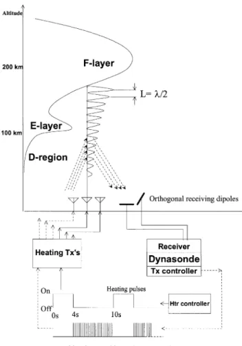
Figure 1 shows schematically the formation of the density irregularities in the standing-wave pattern applied to the situation in Tromsø. The EISCAT heating facility (Rietveldet al., 1993) is used to transmit both the pump wave and probing waves. Since the facility consists of 12 transmitters each connected to its own antenna, it is possible to select a subset of transmitters or two groups of transmitters having different frequencies for the pumping and probing waves. The full power of the facility is not necessary for the success of the API experiments and so reduced power is often used. Selecting fewer than 12 transmitters means that the radiated beam width increases in the north-south plane beyond the normal half-power full width of 15°of the lowest-frequency array (Array 2).
Fig. 1. Schematic diagram illustrating the single-frequency API ex-perimental arrangement at Tromsø. In this arrangement Bragg scattering is in principle possible throughout the whole height region up to the F layer if the irregularities are formed and have a long enough decay time to be probed after the pump has been switched off
The wider beam width has the disadvantage that off-vertical echoes from natural irregularities will be stronger and the API echoes weaker. The API echoes are thought to occur only from the first Fresnel zone overhead.
The receiver for the probing wave is the dynasonde (Wright et al., 1990), an advanced digital HF sounder. Receiving antennas are 22-m-long dipoles which have a gain of about 3 dB and are normally used during stan-dard ionospheric sounding with the dynasonde. The dyn-asonde is operated in a fixed-frequency sounding mode (P-mode) which was designed for partial-reflection work. In this mode 30-ls pulses are transmitted and a 60-kHz
wide filter is used in the receiver to give 4.5-km height resolution from the time of flight. Only in some of the early experiments was a 60-ls pulse used with a 30-kHz
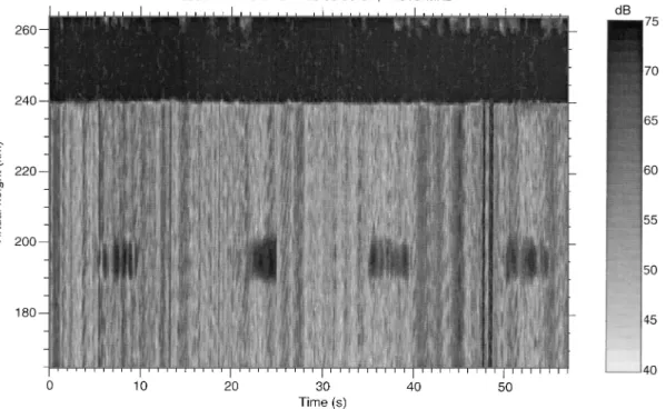
Fig. 2. Grey-scale plot showing the power backscattered by a 4.9128-MHz probing wave with 60-ls pulses while the Heating transmitter was transmitting a 5.423-MHz, X-mode wave of 5-s
duration every 15 s. The vertical resolution is 9 km, determined by the 60ls pulse length and the 30-kHz receiving bandwidth. The dark band above 240 km is the saturated echo from the F layer
sounding. All complex amplitudes in a chosen height range were sampled with 12 bits every 10ls and recorded
on disk. Subsequent analysis enabled the circularly polarised components to be reconstructed.
The ISR data we will use for comparison with the API data were obtained with the GEN-11 experiment, also known as CP-6, on the VHF (224-MHz) radar (Turunen, T., 1986). This 13-bit Barker-coded experiment yields auto-correlation functions of the plasma at 1.05-km range intervals every 10 s from 70- to 113-km range. These are then integrated and analysed to give electron density, Doppler velocity and spectral width. We are only con-cerned with electron-density and velocity results here.
4 F-region echoes
In February 1993 the first experiments were made at Tromsø to determine the feasibility of detecting Bragg scatter off API in the F region using the two-frequency arrangement. The pump wave was on for 5 s every 15 s at 5.423 MHz in the X-mode using 4 transmitters each at 60 kW giving an ERP of about 30 MW, while the probe was at 4.9128 MHz in the O-mode also from 4 transmit-ters at 60 kW each. The probing pulse was 60ls long in
these early experiments and repeated typically every 20 ms. These attempts immediately proved successful, as the range-time-intensity plot in Fig. 2 shows. For this initial experiment the receiving antenna used was in fact the Tromsø University partial-reflection experiment (PRE) antenna array designed for 2.75 MHz. It was felt that this would be more sensitive than the standard long dipoles normally used by the dynasonde, and that this
extra sensitivity would be necessary, although subsequent experiments showed that even simple dipole antennas work well. In the Russian experiments a partial-reflection facility was used for the API probing (Belikovichet al., 1995).
For the experiment in Fig. 2, the data from 4 pulses (80 ms) were collected followed by a gap of 7 pulses (140 ms). Because the resulting periodic time resolution of the data was only 0.22 s, we cannot resolve the temporal variation of the echoes very well. Nevertheless, one can see in the first two heater pulses a broadening of the reso-nance region in the first few seconds. This may be indica-tive of the formation of irregularities in the F region and so this technique could prove to be of value when com-bined with other measurements of the heated region. When Fejeret al. (1984) performed a similar experiment at Arecibo, they found that the ratio of the scattered API power to specularly reflected power ‘‘was about 10~4, considerably higher than the value of about 2.5]10~9
There was another intriguing effect seen in API echoes just below the F layer during the early single-frequency experiments which deserves closer examination. There was a region of backscatter extending 10 km or more below the specular reflection height immediately after heater switch-off and which decayed, apparently moving upwards to the specular reflection level within about 100 ms. Perhaps this was an electron-density stratification in the Airy pattern of the standing HF wave which decayed. The large extent of more than 10 km below the reflection height may have been only an apparent one if the reduction in group delay for frequencies just slightly off the pump frequency really occurs as predicted by Fejer (1983). Although the probing wave was at the same fre-quency as the pump wave, the 60-ls pulse length ensures
that there is significant energy within a several-kHz band-width. We intend to verify this phenomena in the near future. Apart from these preliminary F-region observa-tions, however, we have concentrated on the experiments in the lower ionosphere. The reason is that although with the EISCAT facilities one has generally a very good in-strument to measure F-region parameters at nearly all times, the lower D region can be diagnosed only under special conditions even with such powerful ISR systems.
5 D and E-region echoes
5.1 October—November 1993 measurements
In October 1993, the first successful single-frequency ex-periment for the lower ionosphere was made at Tromsø. Since then we have repeated the experiments at irregular intervals. We present below some characteristics of the echoes, but so far we have not performed any statistical or systematic seasonal studies. In November 1993 we attem-pted to compare API results with those from incoherent-scatter observations of the D region on two days. For both pump and diagnostic pulses we used all 12 transmit-ters at 90 kW each giving 300 MW of ERP. The pump was switched on for either 4 or 26 s (this alternated every 5 min) followed by 4 s of 30-ls diagnostic pulses every
10 ms.
During the first attempt on 16 November 1993 there were strong signals in the VHF-ISR data due to electron precipitation, but as a result the D-region absorption appeared to be too high for the API experiment to work at 4.04 MHz, at least using X-mode for the pump and diagnostic waves, which we invariably did in the early attempts. In fact ionograms made before and after the API experiment showed a lack of X-mode trace but a clear O-mode trace. In retrospect, changing to O-mode operation may have resulted in successful API generation.
The second attempt on 18 November 1993 resulted in excellent API echoes, but the signal-to-noise ratio of D-region signals in the ISR data below 80 km was very low. Figure 3 shows a combined grey-scale and surface plot of some of the API echoes, again obtained with 4.04-MHz X-mode waves. One can see a clear decay of echo strength with time between 77 and 120 km with varying
time-constant. At 94 km there appears to be a sharp minimum in irregularity production. Below this the time-constant is either much longer than the 4 s of sampling which we used, or the irregularity decay is superimposed on a pre-existing natural irregularity which varies little over the 4 s sampled. We have analysed a half-hour inter-val of such data to obtain the amplitude, time-constant and rate of change of phase of the decaying API irregulari-ties. Figure 4 shows a series of amplitude and phase variations (dots) for the data in Fig. 3 together with fitted (solid lines) functions. In the left column an exponential function plus constant baseline is fitted to the amplitude, while in the right column a linear fit was made to the phase. The time-constant of the exponential fit and appar-ent velocity from the linear rate of change of phase are indicated in each fit. We show only every fourth height sampled because there is considerable overlap between gates due to oversampling. The phase fit was made only using those points in the time-series where the amplitude had decreased to 1/e of its initial value for two reasons: to minimise the effect of noise on the fit, and to fit only those points where the API echoes dominate over other echoes from spatially distributed inhomogeneities. The reduced chi-square values were calculated assuming random Gaussian noise. The standard deviations of the random fluctuations in the data were calculated from the point-to-point data differences. The data point-to-points were equally weighted for all these fits: other forms of weighting were tried but made very little difference.
Fig. 3. Grey-scale and surface plot of API echoes between 80 and 120 km from 18 November 1993. The surface plot shows linear amplitude. The X-mode HF pump had been on for 4 s prior to the 0-s tick. The vertical resolution is 4.5 km in these data. Pump and probing waves were 4.04 MHz
The first three panels in Fig. 6 show profiles of API amplitudes, decay time-constants and fitted velocities over 5 min (1145—1150 UT) together with their random error bars. The time-constants below about 105 km show a large variation. They were difficult to fit, partly due to the 4-s sampling window being too short compared to some of the long-lived echoes which appear to be a combi-nation of API and partial reflections. Some of the vari-ation, particularly in the velocities, may be caused by
&&&&&&&&&&&&&&&&&&&&&&&&&&&&&&&&&P Fig. 4. A profile of API echo amplitude and phase fits from the echoes in Fig. 3. The time-constant (¹
Fig. 6. Profiles of amplitude, decay time-constant and derived verti-cal velocities from API together with their random error bars. Data from simultaneous incoherent-scatter-radar measurements are some
vertical velocities (asterisks) and electron density (rightmost panel); 18 November 1993, 1145—1150 UT
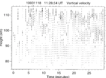
Fig. 5. Vector plot of vertical velocities derived from the rate of change of phase as illustrated in Fig. 4, 18 November, 1993, 1129—1200 UT. There are clearly coherent regions of both upwards and downwards velocity evident. The distance between vectors cor-responds to 10 m s~1
wave activity. To show that the variation in velocity really is due to wave activity, a FFT was performed on the time-series of velocities at a particular height. For heights in the range from about 80 to 95 km there was generally a decrease in power from 0 to 0.005 Hz followed by a constant power level for higher frequencies. The cut-off at 0.005 Hz could correspond to the gravity-wave spectrum cut-off at a Brunt-Va¨isa¨la¨ period of about 3.5 min.
data. The signal-to-noise ratio of the ISR data was too poor to enable good velocity estimates to be made with the intrinsic 1.05-km height resolution. The autocorrela-tion funcautocorrela-tions from three gates were therefore averaged in height and integrated for 5 min to produce these data, but the error bars are still very large. The agreement between the two data sets is not so good in magnitude but the sign of the velocities agrees (positive velocity means upwards). It is difficult to reach any firm conclusion on the reliability of derived vertical-wind motions from the API technique based on this comparison. Nevertheless, it does emphasise the complementary conditions necessary for the two tech-niques to produce data. Velocities can be derived with excellent time resolution (tens of seconds) and good height resolution (about 5 km) at times when ISR measurements are of little use.
The correctness of the sign of the velocities derived from the API measurements was verified independently by comparing the velocities derived from echoes off a sporadic-E layer which was descending steadily between about 1000 and 1030 UT during the experiment. This layer was seen by both the dynasonde/heater radar as well as the ISR. The velocity derived from the rate of phase change was consistently negative (downwards) and of the correct order of magnitude as the average rate of descent (about 2 m s~1) of the layer as obtained from the time-of-flight measurements.
5.2. Sources of error in velocity determination
The velocity we derive from the rate of change of phase has a contribution from the different decay rates of the irregularities as a function of height within the volume contributing to the Bragg-scattered signal. One can look at this as a shift in the effective height or centre of gravity of the scattering volume as the height of main contribu-tion to the scattering changes. To estimate quantitatively this effect we have used the measured amplitudes and time-constants to model the irregularity decay and calcu-late the scattered signal on the ground as a sum of indi-vidual phasors from each plane in the Bragg-scattering lattice. The results are not plotted here, but it is sufficient to note that the maximum contribution to the velocity from this effect is about 0.1 m s~1 for the data of 15 September 1994, now shown.
5.3. September 1994 measurements
Further simultaneous VHF-ISR and API measurements were made on 15 September 1994. Ten transmitters of 80 kW each, giving an ERP of about 200 MW, were used for the API experiment. Because we had observed rather long decay times in several previous experiments, and better to determine the natural background echo vari-ation, we used a longer 16-s interval of probing after a 4-s pump. On this occasion no API echoes were obtained at first using an X-mode pump and probe waves. Suspecting that absorption was too high, we changed at 1216 UT to O-mode for both the 4.04-MHz pump and probe waves,
which resulted in good API echoes. These echoes ex-tended below the 67-km lower sampling boundary which we were using, so we decreased the starting height and obtained echoes from about 52 km upwards, as is shown in the combined surface and grey-scale plot in Fig. 7. The API signals are clearly much weaker than those in Fig. 3. Two main regions of decaying echoes are seen above 96 and below 72 km, respectively, with a narrow region of what are probably partial reflections from natural irregu-larities between 86 and 95 km. Partial reflections are com-monly seen at these heights and the reader is referred to Evans (1974), Dieminger and Schlegel (1976) and refer-ences therein for a more extensive description of these echoes and the technique.
Figure 8 shows the amplitude and phase fits to these data for the first 4 s of each time-series. In general the fits are very good and repeatable between heater pump pulses which were 20 s apart. Although the linear fits to the phase are very good, the resulting vertical velocities show a bias of about!4 m s~1over the whole profile, which is diffi-cult to explain as a neutral wind. Looking at the sub-sequent fits (Fig. 10), we see the bias may be smaller but is still negative over the whole range. We have no explana-tion for this bias.
The signal-to-noise ratio of the ISR signals, which had generally been low since the beginning of the experiment at 1100 UT, suddenly increased between about 1220 and 1250 UT as some electron precipitation occurred. Figure 9 shows for the interval 1220—1230 UT mean profiles of the API amplitude, time-constant and derived vertical velocity, together with bars showing their standard devi-ation. The standard deviation is not to be regarded as an error bar associated with a typical measurement but a measure of the actual variation of the quantity involved. The asterisks show the vertical velocities from the VHF radar, this time with the intrinsic 1.05-km resolution. The error bars of the VHF velocities are very small in compari-son to the 18 November 1993 data: they are of the order of the size of the asterisk. Again illustrating the comp-lementarity of the conditions required for the two experi-ments, API signals were weak and the resulting data were sparse. Nevertheless, there are enough values for a reaso-nable comparison over the limited height range from about 72 to 97 km. The velocities from the two techniques agree with each other to within a metre per second at some heights but differ by several metres per second at others. A difference of a few metres per second is large for vertical velocities. In this comparison we believe that the ISR velocity data are reliable because of the rather good signal-to-noise ratio, and that the API-derived velocities above 75 km may be in error, since the amplitudes of the API echoes were weak and perhaps influenced by partial-reflection echoes.
Fig. 7. Grey-scale and surface plots of API echoes extending down to 52 km on 15 September 1994. The surface plot shows linear amplitude. The pump and probing HF waves were 4.04 MHz and O-mode during these measurements. The pump had been on for 4 s prior to the 0-s tick. The weaker echoes between 85 and 95 km are thought to be natural partial reflections
The dashed line shows the corresponding density profile for the interval 1240 to 1250 UT, showing that conditions were stable. The tilted antenna meant, however, that the velocity measurements now contained a large horizontal component of the wind which made direct comparisons with API-derived vertical winds impossible. Such hori-zontal velocities may be of interest in future, more detailed studies of the possible effect of wind shear-induced turbu-lence on API echoes.
There is a sporadic-E layer visible in the electron den-sity profiles at 102.5-km altitude. This was also observable
in the API data, but was not included in the analysis of the API decays. Such a layer should be of use in calibrating the height determination of the API data. The strong saturated echoes of the HF wave from this layer, together with the fading and variability, were such that the echo appeared very broad, so that accurate determinations were difficult with this precision. Other independent calib-rations confirm that the dynasonde-derived heights pre-sented here are correct to within about a kilometre.
Fig. 8. A profile of amplitude and phase fits to the data in Fig. 7 with the same format as Fig. 4. No fit was attempted at 91 km
Fig. 9. Mean profiles of API amplitude, decay time-constant and vertical velocity shown with their standard deviations, integrated over 1220—1230 UT on 15 September 1994. The velocities indicated byasterisksare from a simultaneous incoherent-scatter experiment
as are the raw electron densities in theright-hand panel. The densities shown by the solid line are from a vertical antenna position (1220—1230 UT), while those shown by thedashed lineare from an elevation 67°to the north (1240—1250 UT)
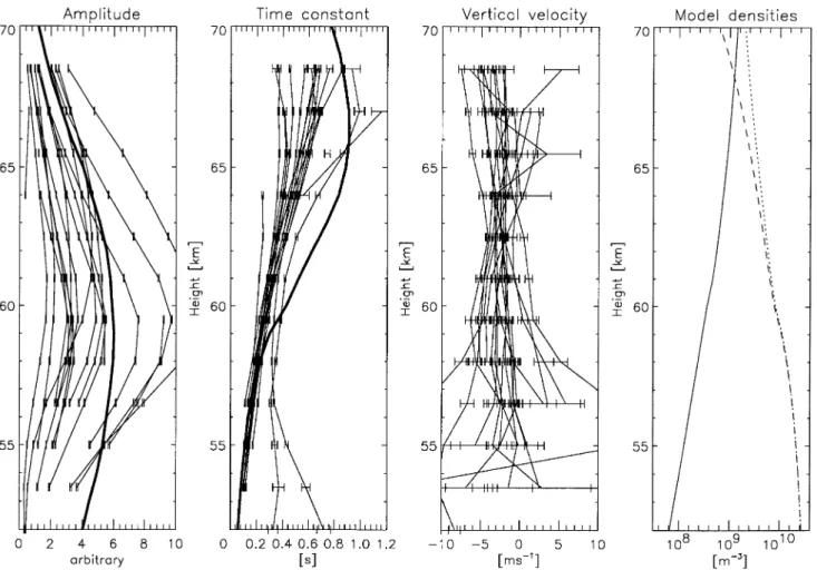
precipitation from about 1310 to 1314 UT where densities only below 80 km were enhanced. This brief event was also seen by a nearby imaging riometer as a localised patch of absorption. Excellent API signals were obtained from 1314 UT onwards (there were no API data taken during the relativistic precipitation burst) with API signals covering the region 57—77 km, as we have seen. In Fig. 10 we show the individual ampli-tudes, time-constants and velocities derived during the interval 1326—1332 UT, with the bars showing the errors of the fitted values assuming Gaussian noise. The time-constant shows relatively little variation, while the velo-city shows more variation and the amplitude shows the most, as one might expect, since the amplitude is depen-dent on so many propagation conditions. The time-con-stant might be expected to remain largely a property of the ionospheric composition (see Sect. 6) and could be fairly constant over 6 min, while the velocity may be expected to be more sensitive to wave activity in the neutral wind.
5.4. Strength of echoes and conditions
Belikovich and Benediktov (1986a) report the amplitude of the D/E region API echoes to be 50—80 dB below that of specular reflection. In our experiments we have not measured this carefully, since, in the cases where we have F-region specular reflection, the echoes saturated the re-ceiver. We have examples of API echoes at 100 km being about 20 dB below the saturated F-region echo. Generally we can say that the echo strength is comparable to that of natural partial reflections.
We briefly discuss the question: Is it reasonable to expect detectable irregularities to be produced by the HF-standing-wave pattern at such low altitudes ? Even if there are no other losses, the range squared losses of the HF wave reflecting from about 200 km imply that the standing-wave ripple is no more than about 5% in power. Assume an electron density at 70 km of 1]108m~3and
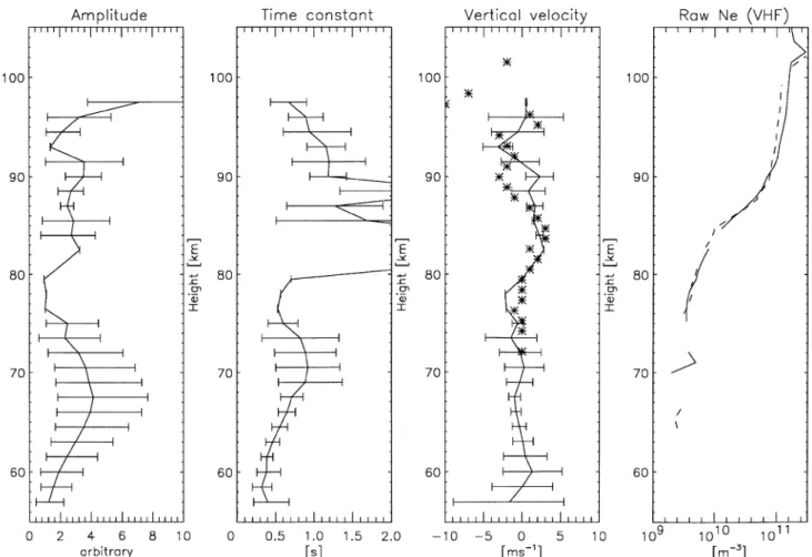
Fig. 10. Profiles of amplitude, decay time-constant and vertical veloc-ity over a 6-min interval on 15 September 1994. Thebarsshow the individual errors of the parameters of the 18 measurements within this time-interval. Thethick linesshow the modelled amplitude and
time-constant from the Sodankyla¨ ion-chemistry model. Thefourth panel shows the electron density (solid line), positive-ion density (dotted line) and negative-ion density (dashed line) used in the model
calculations in Sect. 6 show that this heating effect can cause a 12% decrease in electron density of which only 5% is modulated by the standing wave, which means that the amplitude of the density modulation is 6]105m~3. This causes a change in the refractive index (Dn) at 4 MHz
of 2]10~6. Gardner and Pawsey (1953) argue that it
would suffice to explain 70 km partial reflection echoes (with a typical reflection coefficient of 10~5) if there were an abrupt change of refractive index of only 2]10~5
extending over the sky. An approximately equal echo would be caused by a discontinuity which extended not over the whole sky, but over a substantial fraction of a Fresnel zone (about 3 km in diameter). The API echoes are comparable in strength with partial reflections, as we have seen. So the refractive index change which causes the API is about 1/10 of that necessary to explain partial reflections. There are, however, tens of such layers half a wave-length apart so as to reflect coherently (Bragg scatter), so that it may be reasonable to expect a total reflectivity about the same as that for partial reflections. There are several uncertainties involved here. The reflec-ted wave may be weaker through absorption, but the temperature and resulting density change may well be
greater than assumed here. The electron density may be an order of magnitude higher as it was in the experiment from 15 September 1994, so that Dn would already be
2]10~5. Another complicating factor is that the refrac-tive index perturbations are in layers about a quarter-wavelength thick rather than as the single abrupt layer assumed by Gardner and Pawsey (1953).
In most of the above experiments we used X-mode heating and probing so as to avoid the perturbations to the F region known to occur with O-mode heating, such as the formation of electrostatic plasma waves leading to anomalous (non-Ohmic) heating, density striations and anomalous absorption of other HF waves (see Stubbe, 1996, and references therein). X-mode also has the advant-age that one may still be able to form a standing-wave pattern when ionospheric critical frequencies are so low thatf
oF2is below the lowest usable heater frequency of
4 MHz, whereasf
xF2can be above the heater frequency.
the first time we tried O-mode on 15 September 1994 we saw echoes at the extremely low altitudes of 55 km, as shown in Fig. 7.
5.5 Effects of interfering echoes
In the intensity plot in Fig. 7, API echoes can be seen decaying above and below another relatively constant echo covering the height range 86—93 km. This slowly varying echo is probably a partial reflection which is not unusual at these altitudes. In some cases the API and the natural echoes are so close that interference between them occurs, making the deduction of time-constant and phase derivative difficult. Either analysis of API signals for de-termination of ionospheric parameters must be restricted to cases where the API-signal-to-noise ratio is sufficiently large, as has been done by previous workers (Belikovich and Benediktov, 1986a), or advanced signal subtraction techniques must be used to subtract the natural echoes. The latter approach may be impractical since the time-constant for the natural echo variation appears to be sim-ilar to that for the API.
When natural partial reflections are present, it is often possible to derive an apparent velocity from the rate of change of phase, which is often constant. Such velocities may, however, include non-vertical components, since the reflections may be off localised scattering regions within the heater-illuminated beam, which is 15° wide in the east-west direction or even larger in the north-south direc-tion when not all transmitters are used. Care needs to be taken, therefore, in separating natural and artificially in-duced echoes when attempting to deduce vertical vel-ocities.
We have the impression that API echoes do not appear in those height regions, usually below 95 km, where there are partial reflections present. This may be because the turbulent motions associated with the partial reflections prevent the weak horizontal electron-density stratification from forming to a significant extent. On the other hand, API echoes are sometimes observed with non-blanketing sporadic-E layers appearing within the API-echo region, usually at heights above about 100 km.
6 Interpretation of decay times below 70 km
6.1. Time-dependent solution of a detailed ion-chemistry model
In the lower F region and E region, thermal effects are dominant and changes in the ambipolar diffusion coeffic-ient (D) govern the formation and decay of the irregulari-ties. In the lower D region, however, the time-constant for diffusion,q
d, given by (k2D)~1, wherekis the wave
num-ber, becomes large. For example, at 70 km,q
d"140 s for
25-m spatial scales (Belikovich and Goncharov, 1995). Another possible irregularity production mechanism at these heights is electron recombination, which also has a time-constant which is comparably long, given by (2a
%&&N)~1, whereNis the electron density anda%&&is the
effective recombination rate which is electron-temper-ature dependent. Because of dynamic changes in the iono-sphere it seems unlikely that the standing-wave pattern is stationary enough over such long time-scales to produce periodic irregularities by either of these two mechanisms. There is, however, a mechanism which does have a short enough time-constant (0.1—1 s) to produce API at heights of the lower D region, and that is electron attachment to oxygen molecules (Tomko et al., 1980). Thus the API technique should be useful for investigations of the nega-tive ion chemistry.
We use a model scheme to answer the following ques-tion: What is the exact chemical response of the iono-sphere at D-region altitudes in a typical API experiment, where heating is on for 4 s and off for 16 s ? The electron temperature can increase through HF heating by about an order of magnitude in the D region on time-scales from 10ls at 60 km to about 1 ms at 90 km (Tomkoet al., 1980;
Stubbe, 1996). For simplicity, let us first assume that the electron temperature is doubled in the time-scale of mil-liseconds or less when heating is switched on. Since the chemical response times are known to be much slower, we may simply calculate the time behaviour in a detailed ion-chemistry model, during one API experiment cycle, by studying what happens to the equilibrium ion concentra-tions when electron temperature is suddenly doubled for 4 s and then suddenly halved back to the normal value for 16 s. In actual calculations we use a representative altitude profile of electron-temperature increase due to the heat-ing. Electron temperature is assumed to be doubled at the altitude of 70 km. At lower altitudes, a cubic spline interpolation is used so as to give an increase in electron temperature by a factor of 1.2 at the altitude of 50 km.
We use a detailed D-region ion-chemistry model with 55 ion components, of which 36 are positive and 19 are negative. This model, the Sodankyla¨ ion-chemistry (SIC) model, was developed as an alternative approach to those D-region ion-chemistry models, which combine the more doubtful chemical reactions to effective parameters whose values are set against experimental data. The original version of the program included a detailed chemical scheme, in a conceptually simple model, for equilibrium calculations in the altitude range from 70 to 100 km [see e.g. Burnset al., (1991); Turunenet al. (1995) also includes some background information on the model and its ap-plications]. In the present version of the model, the selec-tion of ions is extended to include more positive cluster ions, a selection of simple negative cluster ions and also chlorine ions (for a list of ions, see Turunenet al., 1995), so that the model is aimed to be representative for the alti-tude range from 55 to 100 km in daylight conditions. Since the altitude coverage of the API data, relevant to this comparison, is from 52 to 77 km, we use the same choice of ions in the model calculations down to 50 km, although important, higher-order negative cluster ions are known to exist at lower altitudes. Now we introduce time depend-ence into the model by solving the continuity equation in the form
where N is a vector of unknown ion concentrations,
Ca matrix of production and loss rates due to the mutual
reactions between ions andQis a vector of production rates in primary ionisation processes and in some specific reac-tion types. Equilibrium may be solved from Eq. 1 by setting
LN/Lt"0, and using, e.g., the Newton-Raphson method
(for details see Turunen et al., 1995). Starting from the equilibrium solution of the ion concentrations, we advance the concentrations in time, by taking small time-steps ac-cording to an implicit differencing method (see Presset al., 1989, p. 631). For each time-step, a set of linear equations has to be solved. The neutral atmosphere is taken from the MSIS-90 model. Those minor constituents which are not covered by MSIS-90 are taken from Shimazaki (1985). The primary ionisation is considered to be caused by cosmic rays and solar illumination only. The right-hand panel in Fig. 10 shows the model electron, positive-ion and nega-tive-ion densities. The model electron density at 70 km is 1.4]109m~3 which is in reasonable agreement with the
ISR measured density shown in Fig. 9.
As a result of the model calculation we have the time behaviour of each ion concentration during the API cycle. The positive ions are seen to be unaffected by the API heating cycle. The concentration of negative ions responds rapidly to the heating, so that over 4 s a decrease of 12% in electron density is observed in the example case at the altitude of 70 km. When heating is switched off the electron concentration relaxes to the equilibrium value, with a char-acteristic time which can be compared with the measured API signal relaxation times. The most important negative ions, which are responsible for the rapid electron-concen-tration changes, appear to be O~2, CO~3 and CO~4.
The thick solid lines in Fig. 10 are the resulting ampli-tude and decay time-constant calculated from the model. The amplitude, which is calculated in arbitrary units and is simply proportional to the calculated heater-induced electron-density change, shows good agreement with the data, in that it has a maximum at about the same altitude as that of the measured amplitudes. The time-constant also shows reasonable agreement with the data overall. The agreement is excellent below below 60 km, but above that the experimental data tends to be lower than the model values by up to a factor of two.
Time-constants in the height range 50—70 km were also derived by Belikovichet al. (1981), Belikovich and Benedik-tov (1986a) (their Figs. 1—5), Belikovich and Benediktov (1986b) (their Fig. 2) and Terina (1996). These authors also found that above 65 km, the observed time-constants were lower than expected from a simplified scheme of negative ion chemistry. They suggested that this could be explained by turbulence-induced decay of the API. The experimental values they obtained for the summer months are similar to our September values, whereas their winter results show values lower by about a factor of 2. We shall examine the seasonal variation and compare them with the mid-latitude results after we have collected a larger data base.
7 Conclusions and future work
After reviewing previous work from other latitudes we have shown the first echoes from artificial periodic
ir-regularities produced in the auroral ionosphere by a powerful HF wave reflected off the F layer. Both F-region and lower ionospheric echoes down to about 52 km were obtained using simple dipole receiving an-tennas. The D-region echoes have been analysed to obtain time-constants of their decay and vertical velocities. Simultaneous ISR measurements of the electron density and vertical velocity were made by the 224-MHz EISCAT radar so that the latter could be compared with velocities derived from the API technique. The optimum geophysi-cal conditions for the two techniques seem to be com-plementary, such that the ISR gives best results when there is electron precipitation and the HF absorption is higher, whereas the API technique works best when there is lower absorption. As a result, although there is some agreement between the data sets, we do not have simulta-neous good-quality data sets and cannot show that both techniques measure the same quantity, namely vertical neutral wind. Time-series of API-derived velocities from 18 November 1993 do show signatures of vertical winds, in that the magnitudes are reasonable, the average value is near zero, and there are signs of gravity-wave fluctuations. Velocity data from a 5-min time-interval and 50—70-km height interval on 15 September 1994, however, show a bias of several metres per second, which is difficult to reconcile with vertical winds. Obviously more work is needed in the area of data selection and analysis and theory of API formation, in order reliably to derive vertical winds.
The parameter obtained from the API measurements in the lower D region which one would expect to vary least is the decay time-constant. A completely independent calculation of the predicted time-constant obtained from a complex ion-chemistry model of the lower D region shows reasonable agreement with the measurements. This indicates that we have a good basis for making more refined comparisons between this model and experimental API measurements as well as ISR measurements.
We have shown the feasibility of making API measure-ments in the high-latitude ionosphere and that it can be done with relative ease. Future experiments at Tromsøwill be made to examine F-region API echoes during heating experiments in more detail, to determine the structuring of electron density just below the reflection height.
A proper partial-reflection experiment should be per-formed at the same time as the API experiment to provide further information on D-region electron densities, since the partial-reflection technique is far more sensitive than the ISR technique at these heights. This knowledge should be combined with a self-consistent calculation of the heat-ing effect, which would provide a more accurate input to the ion-chemistry model than that used here.
Acknowledgements. The EISCAT Scientific Association is sup-ported by the research councils of France, Finland, Germany, Nor-way, Sweden and the United Kingdom. We thank J. Ro¨ttger for initiating N. P. Goncharov’s involvement, and S. Eliassen and T. Blomstrand for building the hardware involved in interfacing the dynasonde to the Heating transmitters.
References
Belikovich, V. V., and E. A. Benediktov,Investigation of the lower part of the D region of the ionosphere using artificial periodic inhomogeneities,Radiophys.Quantum Electron. (Engl. Transl.),
29,11, 963—973, 1986a.
Belikovich, V. V., and E. A. Benediktov,The influence of temperature on the state of the plasma in the lower part of the D region of the ionosphere, Geomagn. Aeron. (Engl. Transl.), 26, 5, 707—709, 1986b.
Belikovich, V. V., and E. A. Benediktov,Artificial periodic nonunifor-mities in the lower part of the D region at sunset and sunrise,
Geomagn.Aeron. (Engl. Transl.),26,5, 705—706, 1986c.
Belkovich, V. V., and N. P. Goncharov,Ionospheric D-region studies using artificial periodic irregularities, Geomagn. Aeron. (Engl. Transl.),34,6, 787—795, 1995.
Belikovich ,V. V., and E. A. Mareev,Radiowave scattering by artifi-cial quasi-periodic irregularities in the ionosphere,Radiophys.
Quantum Electron(Engl. Transl.),30,631—634, 1987.
Belikovich, V. V., and S. V. Razin, Formation of artificial periodic inhomogeneities in the D region of the ionosphere with attach-ment and recombination processes taken into consideration,
Radiophys.Quantum Electron. (Engl. Transl.),29,187—191, 1986.
Belikovich, V. V., E. A. Benediktov, G. G. Getmantsev, Yu. A. Ignat’ev, and G. P. Komrakov,Scattering of radio waves from the artificially perturbed F region of the ionosphere, JE¹P¸ett. (Engl. Transl.),22,243—244, 1975.
Belikovich, V. V., E. A. Benediktov, M. A. Itkina, N. A. Mityakov, G. I. Terina, A. V. Tolmacheva, and B. P. Shavin,Scattering of radio waves by periodic artificial ionospheric irregularities,
Radiophys. Quantum Electron. (Engl. Transl.), 20, 1250—1253, 1977.
Belikovich, V. V., E. A. Benediktov, and G. I. Terina,Formation of quasi-periodic artificial inhomogeneities in the ionosphere,
Radiophys.Quantum Electron. (Engl.Transl.),21, 10, 985—988, 1978a.
Belikovich, V. V., E. A. Benediktov, M. A. Itkina, G. I. Terina, and A. V. Tolmacheva, Ionospheric electron density measurement using radio-wave scattering from artificial plasma inhomogenei-ties,Radiophys.Quantum Electron. (Engl. Transl.),21,8, 853—854, 1978b.
Belikovich, V. V., E. A. Benediktov, T. L. Gulyeva, and G. I. Terina,
Determination of electron density profile from the resonance scatter of radio waves and vertical sounding ionograms,
Geomagn.Aeron. (Engl. Transl.),19,6, 681—683, 1979.
Belikovich, V. V., E. A. Benediktov, S. A. Dmitriev, and G. I. Terina,
Plasma artificial periodical irregularities in the lower ionospheric D-region, Radiophys. Quantum Electron. (in Russian), 24, 7, 905—908, 1981.
Belikovich, V. V., E. A. Benediktov, and G. I. Terina,Diagnostics of the lower ionosphere by the method of resonance scattering of radio waves,J.Atmos.¹err.Phys.,48,11—12, 1247—1253, 1986.
Belikovich, V. V., E. A. Benediktov, and N. P. Goncharov,Vertical motions in the ionospheric D and E regions,Geomagn.Aeron. (Engl. Transl.),31,2, 301—303, 1991.
Belikovich, V. V., E. A. Benediktov, V. D. Vyakirev, Yu. N. Grebnev, and A. V. Tolmacheva,Electron-concentration profile measure-ments in the D and E regions of the ionosphere by the methods of partial reflection and resonance scattering of radio waves,
Geomagn.Aeron. (Engl. Transl.),33,1, 121—122, 1993.
Belikovich, V. V., E. A. Benediktov, and A. V. Tolmacheva,A method to determine a vertical profile of the atmospheric temperature using artificial periodical irregularities of the ionospheric plasma,
Geomagn.Aeron. (Engl. Transl.),34,1, 115—117, 1994.
Belikovich, V. V., E. A. Benediktov, and A. V. Tolmacheva, Measure-ments of electron density profiles in the ionosphere using artifi-cial periodic inhomogeneities, in ¹he ºpper Mesosphere and ¸ower¹hermosphere:A Review of Experiment and¹heory,Geo
-phys.Monogr. 87, AGU, Washington, DC, 251—254, 1995.
Burns, C. J., E. Turunen, H. Matveinen, H. Ranta, and J. K. Har-greaves,Chemical modelling of the quiet summer D and E re-gions using EISCAT electron density profiles, J.Atmos.¹err.
Phys.,53,115—134, 1991.
Dieminger, W., and K. Schlegel,Manual of Ionospheric Absorption Measurements(Ed. K. Rawer), World Data Center A, Boulder, Colo., pp. 164, 1976.
Evans, J. V., Some post-war developments in ground-based radiowave sounding of the ionosphere,J.Atmos.¹err.Phys.,36, 2183—2234, 1974.
Fejer, J. A.,Method of remote sensing of horizontal stratification due to an ionospherically reflected powerful radio wave,J.Geo
-phys.Res.,88,489—492, 1983.
Fejer, J. A., F. T. Djuth, and C. A. Gonzales,Bragg backscatter from plasma inhomogeneities due to a powerful ionospherically reflec-ted radio wave,J.Geophys.Res.,89,9145—9147, 1984.
Gardner, F. F., and J. L. Pawsey,Study of the ionospheric D region using partial reflections,J.Atmos.¹err.Phys.,3,321—344, 1953.
Gershman, B. N., and Yu. A. Ryzhov,Turbulent spreading of artifi-cial periodic inhomogeneities in the lower ionosphere,
Radiophys.Quantum Electron. (Engl. Transl.),26,10, 877—879, 1983.
Grigor’ev, G. I., N. G. Denisov, and V. V. Tamoikin,Effect of ionized component motion on the scattering properties of the iono-spheric grating,Radiophys.Quantum Electron. (Engl. Transl.),33,
3, 195—198, 1990.
Hansen, G., and U.-P. Hoppe, Investigation of the upper meso-spheric dynamics under late polar summer conditions by EIS-CAT and lidar,J.Atmos.¹err.Phys.,58,1—4, 317—335, 1996.
Lapin, V. G.,Self-averaging of the field scattered by artificial peri-odic structure in the ionosphere with turbulent motions,
Geomagn.Aeron. (Engl. Transl.),34,2, 257—261, 1994.
Lapin, V. G. and V. V. Tamoikin,Influence of curvature of the phase fronts of the high-power and probe waves on scattering from an artificial periodic array, Radiophys. Quantum Electron. (Engl. Transl.),27,2, 96—103, 1984.
Press, W. H., B. P. Flannery, S. A. Teukolsky, and W. T. Vetterling, Numerical Recipes in Pascal, Cambridge University Press, Cam-bridge, 1989.
Rietveld, M. T., H. Kohl, H. Kopka, and P. Stubbe,Introduction to ionospheric heating experiments at TromsøPart 1: Experimental overview,J.Atmos.¹err.Phys.,55,577—599, 1993.
Shimazaki, T., Minor constituents in the middle atmosphere, Terra Scientific, Tokyo, D. Reidel, Dordrecht, 1985.
Stubbe, P., Review of ionospheric modification experiments at Tromsø,J.Atmos.¹err.Phys.,58,1—4, 349—368, 1996.
Terina, G. I.,Measurement of electron density in the lower iono-sphere by the method of resonance scattering of radio waves,
Geomagn.Aeron. (in Russian)26,499—501, 1986.
Terina, G. I.,Variations of the lower ionosphere parameters meas-ured by the resonance scattering method,J.Atmos.¹err.Phys.,
58,6, 645—653, 1996.
Tomko, A. A., A. J. Ferraro, H. S. Lee, and A. P. Mitra,A theoretical model of D-region ion chemistry modification during high-power radio-wave heating,J.Atmos.¹err.Phys.,42,273—285, 1980.
Turunen, E., H. Matveinen, J. Tolvanen, and H. Ranta,D-region ion chemistry model,submitted for S¹EP Handbook, 1995.
Turunen, T.,GEN-SYSTEM- a new experimental philosophy for EISCAT radars,J.Atmos.¹err.Phys.,48,777—875, 1986.
Varshavskii, I. I., The influence of striction and thermal effects during the plasma disturbance by a strong radio wave,Geomagn.
Aeron. (Engl. Transl.),18,6, 697—701, 1978.
Wright, J. W., P. N. Collis, T. S. Virdi, and R. I. Kressman,A com-parison of plasma densities by EISCAT and the Dynasonde from auroral altitudes: evidence of intense structure,J.Atmos.¹err.
Phys.,52,289—303, 1990.