J. Braz. Comp. Soc. vol.12 número4

Frequency Domain Concurrent

Channel Equalization for

Multicarrier Systems

Fábio D’Agostini

1

, Sirlesio Carboni Júnior

1

, Maria C. F. De Castro

1

& Fernando C. C. De Castro

1

.

1

Department of Electrical Engineering Wireless Technologies Research Center - CPTW Pontifical Catholic University of Rio Grande do Sul

Av. Ipiranga 6681 Phone: +55 (51) 33203500 sn: 4403 Zip 90619-000 – Porto Alegre - RS - BRAZIL

[email protected]—[email protected]—[email protected]—[email protected]

Abstract

Receivers for wireless Orthogonal Frequency Division Multiplexing (OFDM) systems usually perform the channel estimation based on pilot carriers in known positions of the channel spectrum. Interpolation between pilot carriers is applied to determine the channel transfer function in all carrier frequencies. Channel variations along time are compensated by means of interpolation between successive channel estimates on the same carrier frequency. However, not rarely, the fast channel variations exceed the time interpolator capability, as is the case for mobile operation. In this article we present a new channel compensation technique based on the concurrent operation of two stochastic gradient time-domain algorithms, one which minimizes a cost function that measures the received signal energy dispersion and other which minimizes the Euclidean distance between the received digital modulation symbols and the ones in the reference constellation assigned to each OFDM sub-channel. Results show that the new technique advantageously improves the system robustness to fast channel variations since, with a low computational cost, it

dramatically reduces the demodulator symbol error rate even when the receiver is operating in an intense dynamic multipath scenario.

Keywords: Concurrent, Equalization, Broadcast, Modulation,

Pilots, Multicarrier.

1.

I

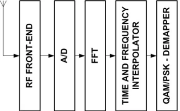
NTRODUCTION

The CE is a time domain adaptive algorithm which was originally proposed for single carrier systems [2]. In this work we extend the use of the CE to multicarrier OFDM systems by applying the same principle in the frequency domain. Figure 1 shows the simplified model for a typical OFDM demodulator and the usual symbol aided channel estimation scheme [5]. Reference symbols – so-called pilot symbols – are applied to pilot sub-channels (carriers) before the IFFT at the transmitter. At the receiver, the pilot sub-channels in the FFT output are estimated by the received known pilot symbols at its respective frequencies of the channel spectrum.

Interpolation is then applied in time direction and in frequency direction so that all

N

_C OFDM sub-channels transfer functions

H

_n

(

f

,

t

)

,

n

=

0

,

_L

,

N

_C

−

1

, are frequency compensated taking into account the channel dynamic behavior [1].

Figure 1: Simplified model for an OFDM demodulator. Among the several existing interpolation techniques, the Wiener Filter presents one

of the lowest interpolation errors [9].

In this work we add a concurrent blind deconvolution algorithm to the time interpolation performed in each OFDM sub-channel. This blind stochastic algorithm follows the approach adopted for the Concurrent Equalizer, as presented in [2]. Results show not only a remarkable robustness increase under dynamic multipath operation as well a complexity reduction in the channel estimation procedure.

2.

S

YMBOL AIDED

C

HANNEL

E

STIMATION

In order to properly estimate the channel transfer function

H

(

f

,

t

)

by means of interpolation, the distance between adjacent pilot symbols in frequency and time needs to be respectively small with respect to the expected channel multipath delay and to the expected channel Doppler frequency [5].

In an OFDM receiver, function

H

(

f

,

t

)

is estimated in discrete frequency domain, since the estimation is performed for each received OFDM symbol. Thus, the

duration of one OFDM symbol is the minimum distance between two adjacent pilot symbols in time direction. Actually,

H

(

f

,

t

)

is estimated in a two-dimensional discrete frequency and time grid, with the channel transfer function being denoted by

H

_n,i and its estimates being denoted by

H

ˆ

_n,i,

n

=

0

,

L

,

N

_C

−

1

and

1

,

,

0

−

=

N

_S

i

L

, where

N

_C is the number of carriers (sub-channels) per OFDM symbol and

N

_S is the number of OFDM symbols per OFDM frame.

Figure 2 shows an example of the grid resulting after the FFT for a received OFDM frame. Notice the rectangular arrangement of the symbol pilots, which denotes it as a rectangular pilot grid. The distance between two pilot symbols in frequency direction is

N

_f carriers. The distance between two pilot symbols in time direction is

N

_t OFDM symbols.

The implementation of a control system as a program with concurrent objects is based on concurrency models of multithreading, which allows the representation of a system as a network of cooperative elements, in this case the Agents. The use of the same base class for deriving all classes guarantees the uniformity of interface for all system elements, thus making the program easier and minimizing implementation errors.

Figure 2: Two-dimensional discrete frequency and time grid for

(

f

t

)

H

,

estimation. In such discrete domain, the channel transfer

function is denoted by

H

_n,i. Notice that

N

_f

=

4

and

N

_t

=

5

in

Each IQ symbol in the received grid is given by

i n i n i n i

n

H

S

N

R

_,

=

_{, ,}

+

_, (1)

where

S

_n,i is the IQ symbol applied to the

n

th carrier of the

i

th OFDM symbol at the transmitter and

N

_n,i is the respective additive channel noise.

Let

n

'

and

i

'

respectively be the frequency and time indexes in the grid for which the OFDM transmitter assigns a pilot symbol

S

_n,'i'. These indexes are given by

f

pN

n

'

=

(2)

t

qN

i

'

=

(3)

with

0

,

,

_⎥

−

1

⎥

⎤

⎢

⎢

⎡

=

N

_C

/N

_f

p

_L

, where

N

_f is the spacing between two pilot symbols in frequency direction,

1

/

,

,

0

_⎥

−

⎥

⎤

⎢

⎢

⎡

=

N

_s

N

_t

q

L

, where

N

_t is the spacing

between two pilot symbols in time direction, and

⎡ ⎤

⋅

is the operator which returns the smallest integer larger than or equal to its argument. Notice we are assuming here that the first pilot symbol in the grid is located at the first carrier of the first OFDM symbol in an OFDM frame. Thus, the number of pilot symbols in an OFDM frame is given by

⎥

⎥

⎤

⎢

⎢

⎡

⎥

⎥

⎥

⎤

⎢

⎢

⎢

⎡

=

t S f C grid

N

N

N

N

N

(4)

Let

H

n,'i'

(

be the channel transfer function estimates for those grid positions which contain a pilot symbol

S

_n,'i'. Since all pilot symbols are known at the receiver,

H

(

_n,'i' can be obtained from (1):

' , '

' , ' ' , ' ' , '

' , ' ' , '

i n

i n i n i n

i n i n

S

N

H

S

R

H

(

=

=

+

(5)

However, in order to properly minimize the multipath effects in frequency domain, an OFDM receiver has to estimate the channel transfer function in all carrier frequencies between two pilot symbols spaced by

N

_f in frequency direction and not only in those carrier frequencies for which the OFDM transmitter assigns a pilot symbol. Further, the channel usually presents a dynamic behavior so that its transfer function changes with time.

Thus, the OFDM receiver has to estimate the channel transfer function in all OFDM symbols between two pilot symbols spaced by

N

_t OFDM symbols in time direction.

Therefore, it is clear the need for some interpolation procedure between adjacent pilot symbols in time and in frequency. Indeed, the estimate of the complete channel transfer function for the OFDM frame represented in the grid is obtained by interpolating

H

(

_n',i' samples so that we can obtain

H

ˆ

_n,i not only in grid positions which contain pilot symbols

S

_n,'i' but also between them:

{

∑

}∈

=

i n i n

i n i n i n i

n

H

H

,

' ',

' ', , ', ', ,

ˆ

ψ

ω

(

₍₆₎

where

ω

_n,'i,'n,i is the two-dimensional (time and

frequency) impulse response of the interpolating filter and i

n,

ψ

is the index subset obtained from the grid samples

' ,'i n

H

(

which are in fact used to obtain

H

ˆ

_n,i. The adoption of an index subset

ψ

_n,i – instead of the whole set of indexes of

H

(

_n,'i' – for the estimation of a particular

i n

H

ˆ

_, is justifiable since correlation is significant only for samples of

H

(

_n,'i' closed enough to

H

ˆ

_n,i in time and frequency, for a given particular grid coordinate

( )

n

,

i

. Notice that the number of filter coefficients

N

_tap is given by

{ }

ni grid

tap

N

N

=

#

ψ

_,

≤

(7)

where

#

{}

⋅

is the operator which returns the cardinality of

its argument set. In Figure 2, for example,

N

_grid

=

12

and

N

tap

=

4

.

In practice, however, due to the high computational cost of a two-dimensional interpolating filter, the two-dimensional interpolation process is decomposed in two cascaded one-dimensional interpolation filters working sequentially [8]. In general, interpolation is first performed in time direction and then subsequently in frequency direction. Firstly, for a given frequency index

n

′

to which a pilot symbol is assigned, the estimation of i

n

{ }

∑

∈ ′ ′

=

i n i i n i i i n

H

H

, ' ' , ', ,

ˆ

ψ

ω

(

₍₈₎

Subsequently, for a given time index

i

, the estimation of

H

ˆ

_n,i for a particular frequency index

n

is performed by a frequency direction interpolation filter with impulse response given by coefficients

n n',

ω

, where

{ }

n

′

∈

ψ

_n,i. Notice that, since the

H

ˆ

_n′_,i estimates from (8) are obtained for all frequencies

n

′

to which a pilot symbol is assigned, they can be used with any given time index

i

as pilot symbol references in the subsequent frequency direction interpolation: { }

∑

∈ ′

=

i n n i n n n i n

H

H

, ' , , ' ,

ˆ

ˆ

ψ

ω

₍₉₎

The time direction filter coefficients

ω

_i',i and the frequency direction filter coefficients

ω

_n',n are obtained from the Wiener- Hopf solution [5][8][9]. For the time domain interpolation we have

t t t

P

1 −

=

R

ω

(10)

where

ω

_t is the vector whose

N

_tap components are the time direction filter coefficients

ω

_i',i, i.e.,

ω

_t

=

[

ω

_i′,i

]

, with

i

being the particular time index for which

H

ˆ

_n′,i is estimated for a given frequency index

n

′

and

1

,

1

,

0

−

=

′

N

_tap

i

L

, with

N

_tap

=

N

_{grid_t}, where t

grid

N

_{_} is the adopted number of pilot symbols in time direction for the interpolation procedure.

t

P

in (10) is the vector defined by

P

_t

=

[

θ

_i′_,i

]

, which

results from the time direction cross-correlation between the channel transfer function values and its estimates at time positions corresponding to pilot symbols, and whose

tap

N

components

θ

_i′_,i are given by

(

)

(

)

(

)

S

D S D i i

T

i

i

f

T

i

i

f

′

−

′

−

=

′

π

π

θ

2

2

sin

, ₍₁₁₎

where

T

_S is the duration of one OFDM symbol including the guard interval and

f

_D is the maximum expected Doppler shift in the channel [5].

t

R

in (10) is the matrix defined by

R

_t

=

[

φ

_i′_,i′′

]

,

which results from the time domain auto-correlation between the channel transfer function values at time positions corresponding to pilot symbols, and whose

tap tap

N

N

×

elements

φ

_i′,_i′′ are given by

(

i

i

)

s n i i i

i′ ′′

=

′ ′′

+

δ

′

−

′′

σ

σ

θ

φ

₂ 2 , , (12)

where

θ

_i′,i′′ is given by (11) with the proper index replacement,

δ

( )

⋅

is the delta-Kronecker impulse,

σ

_n2 and

σ

_s2 are respectively the AWGN noise power and the signal power [8].

For the frequency direction interpolation we have

f f f

P

1 −

=

R

ω

(13)

where

ω

_f is the vector whose

N

_tap components are the frequency direction filter coefficients

ω

_n',n, i.e.,

]

[

_n,n f

=

ω

′

ω

, with

n

being the particular time index for

which

H

ˆ

_n,i is estimated for a given time index

i

and

1

,

1

,

0

−

=

′

N

_tap

n

_L

, with

N

_tap

=

N

_{grid_f} , where f

grid

N

_{_} is the adopted number of pilot symbols in frequency direction for the interpolation procedure.

f

P

in (13) is the vector defined by

P

_f

=

[

θ

_n′_,n

]

,

which results from the frequency direction cross-correlation between the channel transfer function values and its estimates at frequency positions corresponding to pilot symbols, and whose

N

_tap components

θ

_n′_,n are given by

(

)

(

)

(

)

S

S n n

F

n

n

F

n

n

′

−

′

−

=

′

πτ

πτ

θ

2

2

sin

, (14)

where

F

_S is the carrier frequency spacing and

τ

is the maximum expected delay spread in the channel [5].

f

R

in (13) is the matrix defined by

[

' ''

]

,n n f

=

φ

R

,

which results from the frequency direction auto-correlation between the channel transfer function values at frequency positions corresponding to pilot symbols, and whose

tap tap

N

(

n

n

)

s n n n n

n′ ′′

=

′ ′′

+

δ

′

−

′′

σ

σ

θ

φ

₂

2

,

, (15)

where

θ

_n′,n′′ is given by (14) with the proper index replacement [8].

The new channel compensation technique presented in this article is based on the CE algorithm, which is a concurrent time direction adaptive algorithm briefly described in the introduction section of this article. In the present work, the CE performs a further adjustment on the channel transfer function estimates obtained from a linear interpolation procedure between two adjacent pilot symbols in frequency direction. The reason for the adoption of linear interpolation instead of Wiener filter interpolation is twofold. First, the linear interpolator complexity is quite lower than the Wiener filter complexity. Second, the concurrent time domain channel compensation perform a local channel estimation, local in the sense that it ignores dependencies among pilot symbols far from each other. Thus, if initialized by estimates that result from Wiener filter interpolation, the concurrent time direction local compensation is “perturbed” by non-local pilot symbols, which might start the gradient in a less optimal descent path.

In order to keep spectral uniformity [1], this work adopts a scattered pilot symbol grid as shown in Figure 3, instead of the fixed pilot symbol grid of Figure 2.

Figure 3: Two-dimensional discrete frequency and time grid for

(

f

t

)

H

,

estimation, showing the scattered symbol pilot positions and

the interpolation procedure.

When using linear interpolation between two adjacent pilot symbols on the scattered pilot grid shown in Figure 3, the interpolation procedure is similar to the two cascaded one-dimensional interpolation Wiener filters. Firstly, for a given frequency index

n

′

to which a pilot symbol is assigned, the estimation of

H

ˆ

_n′_,i for a particular time index

i

is performed by a time domain linear interpolation procedure:

(

)

','

' ', 1 ' ', ,

ˆ

i n t

i n i

n i

n

H

N

H

H

i

i

H

(

(

(

+

⎟

⎟

⎠

⎞

⎜

⎜

⎝

⎛

₋

′

−

=

+

′ (16)

where

{ }

i

′

∈

ψ

_n,i

. Subsequently, for a given time index

i

, the estimation of

H

ˆ

_n,i for a particular frequency index

n

is performed by a frequency domain linear interpolation procedure. As in the Wiener filter case, since the

H

ˆ

_n′,i estimates from (16) are obtained for all frequencies

n

′

to which a pilot symbol is assigned, they can be used with any given time index

i

as pilot symbol references in the subsequent frequency domain linear interpolation:

(

)

ni

f i n i n i

n

H

N

H

H

n

n

H

_, 1, ,

ˆ

_,

ˆ

ˆ

ˆ

′ ′

+ ′

+

⎟

⎟

⎠

⎞

⎜

⎜

⎝

⎛

₋

′

−

=

(17)

where

{ }

n

′

∈

ψ

_n,i.

Notice that

H

ˆ

_n,i given by (17) yields the estimates of the channel transfer function for all frequencies and time indexes of the OFDM frame represented in the grid. Thus, multiplying (1) by

1

H

ˆ

_n,iwe obtain the first channel compensation for the received OFDM frame:

i n

i n i n i n I

i n

H

N

S

H

Y

, , , ,

,

_ˆ

+

=

(18)

3. C

ONCURRENT

F

REQUENCY

D

OM AIN

E

QU A LI ZA T I ON

The new technique presented in this article proposes a further update in the compensated grid samples

Y

_nI_,i aiming to minimize the dynamic multipath effects, so that the further compensated grid yields

Y

_nII_,i

≈

S

_n,i. Since all channel information stored in the pilot symbol grid has been used as reference to determine

Y

_nI_,i, in order to perform any further update it is necessary to rely on references which doesn’t depend on the pilot symbol grid. The CE, briefly described in the introduction section of this article is a high performance and low complexity blind adaptive algorithm which is perfectly suited for the task of performing a further update on

Y

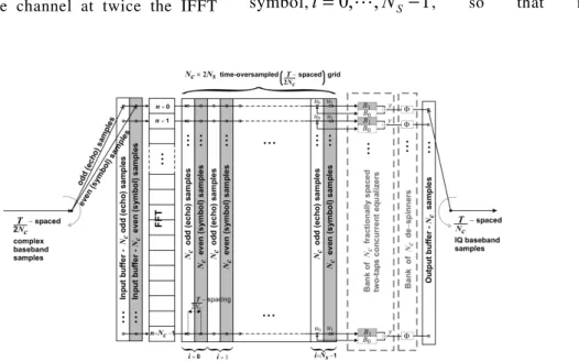
_nI_,i with no dependency on the pilot symbol grid. Figure 4 shows the block diagram for the CE-based channel compensation technique adopted for the deconvolution of each OFDM sub-channel in the OFDM frame, which we called Frequency Domain ConcurrentChannel Equalizer (FDCCE).

With reference to Figure 4, the CE–based channel compensation technique can be described as follows: the receiver samples the channel at twice the IFFT

rate at the transmitter [4], so that after discarding the guard interval, the received

T

/

2

N

_C−spaced complex baseband sequence is stored in two input buffers of size

N

_C at the FFT input. It is assumed that the receiver clock recovery system is such that even-index samples of the received baseband sequence are synchronized to the samples of the IFFT output sequence at the transmitter. Thus each input buffer stores a

T

/

N

_C−spaced complex baseband sequence, one sequence corresponding to even samples and the other sequence corresponding to odd samples. Notice that the odd samples buffer mostly stores information about the multipath channel echo content that occurs in an instant at half the interval between two received

T

/

N

_C−spaced complex symbols.

For the

i

th received OFDM symbol, the FFT reads the even and odd input buffer, performs the time→frequency transformation for each buffer and stores the result respectively in the even and odd partitions of the

i

th column in the time-oversampled grid [4] after de FFT, as shown in figure 4. This procedure is repeated for all

i

th received OFDM

symbol,

i

=

0

,

_L

,

N

_S

−

1

, so that in the

Figure 4: Channel compensation scheme based on a

T

/

2

N

_C−spaced concurrent equalizer (CE) bank with

N

_C equalizers.

T

is the

duration of one OFDM symbol,

N

_C is the number of sub-channels (carriers) per OFDM symbol and

N

_S is the number of OFDM symbols

per OFDM frame. Since the CE is a gradient based blind deconvolution algorithm, each block

Φ

corrects a possible multiple

90

o rotation

end a full OFDM frame is stored in the time-oversampled grid. Then, equation (18) is applied to the even partition of the time-oversampled grid, yielding

I i n

Y

_, as previously explained in Section II.

Subsequently, for each grid coordinate

( )

n

,

i

, the C

N

T

/

2

−spaced samples

u

₀ and

u

₁ are assigned to a sub-channel regressor buffer represented by vector

[

]

T

u

u

u

=

_{0 1} . Notice that position

u

₀ of buffer

u

mostly stores sampled information about the

n

th sub-channel echo content that occurs in an instant at half the interval between two received

T

/

N

_C−spaced complex symbols at the FFT input. Position

u

₁ of buffer

u

stores the compensated IQ symbol

Y

_nI_,i obtained from (18).

For the

n

th sub-channel of the

i

th received OFDM symbol, the CE output

y

is

1 1 0 0

,

u

B

u

B

u

B

Y

_nII_i

=

T

=

+

, where

B

=

[

B

₀

B

₁

]

T is the vector which represents the equalizer filter coefficients. At each iteration

i

, coefficient

B

₀ is adaptively adjusted so that the echo amount

u

₀

B

₀ cancels the intersymbol interference originated by the echo content present in

u

₁

B

₁, driving

u

₀

B

₀

+

u

₁

B

₁ closer to

S

_n,i. Simultaneously, coefficient

B

₁ is

adaptively adjusted so that

1

ˆ

1 , ,

→

b

H

H

i n i n

, also driving

1 1 0 0

B

u

B

u

+

closer to

S

_n,i. After a enough number of received OFDM symbols for which vector

B

is adaptively adjusted at each iteration, the final result is

Y

_nII_,i

=

u

₀

B

₀

+

u

₁

B

₁

≈

S

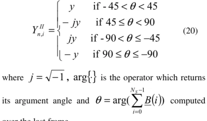
_n,i.

.Actually, since the CE is a gradient based blind deconvolution algorithm, the result for

Y

_nII_,i is of the form ϕ j i n II i

n

S

e

Y

_,

≈

_, (19)

where

ϕ

∈

Φ

,

Φ

=

{

0

o

,

90

o

,

−

90

o

,

180

o

}

, i.e., the II

i n

Y

_, resulting IQ constellation can be rotated of

ϕ

with respect to the reference IQ constellation. Therefore a de-spinning procedure is applied as follows

⎪

⎪

⎩

⎪

⎪

⎨

⎧

−

≤

≤

−

−

≤

<

<

≤

−

<

<

=

90

90

if

45

90

-if

90

45

if

45

45

-if

,

θ

θ

θ

θ

y

jy

jy

y

Y

_nII_i (20)

where

j

=

−

1

,

arg

{}

⋅

is the operator which returns its argument angle and

arg(

( )

)

1 0

∑

− =

=

S N i

i

B

θ

computed

over the last frame.

The adaptive procedure which adjusts vector

B

at each iteration is based on [2], and it aims to perform the stochastic gradient minimization of the CE cost functions for each

n

th sub-channel in the time-oversampled grid of Figure 4, as shown in Table 1.

Table 1: Adaptive procedure applied to each

n

thCE in the time-oversampled grid shown in Figure 4.

Step CE Procedure

1

_i

₌

₀

( )

B

end of previous frame

B

0

=

_{_ _ _}

( )

⎥

⎥

⎦

⎤

⎢

⎢

⎣

⎡

=

_I i n I i n

Y

Y

u

even _ , odd _ ,

0

2

_y

_{( )}

_i

_B

T

_{( ) ( )}

_i

_u

_i

=

3

₍

₎

_{( )}

_{( )}

(

_{( )}

)

_{( )}

i

u

i

y

i

y

i

B

i

B

+

1

=

+

η

_CMA

γ

−

2 *

4

_y

_{( )}

_i

_B

T

₍

_i

_{) ( )}

_u

_i

1

~

₌

₊

5

( )

{

( )

}

{

( )

}

( )

{

}

{

( )

}

⎩

⎨

⎧

≠

=

=

i

y

Q

i

y

Q

i

y

Q

i

y

Q

i

D

_~

if

1

~

if

0

6

(

)

(

)

( )

[

D

i

]

[

{

y

( )

i

}

y

( )

i

]

u

( )

i

i

B

i

B

*

DD

1

Q

1

1

−

−

+

+

=

+

η

7

_Y

II

_y

_{( )}

_i

i n

~

,

=

8

_i

₌

_i

₊

₁

9 _IF

S

N

i

<

GOTO Step 2

In table 1 OFDM symbol counter

i

is reset to

i

=

0

for each new OFDM frame to be compensated by the procedure. Vector

B

=

[

B

₀

B

₁

]

T is initialized at

i

=

0

with the vector

B

value which results at the end of the CE procedure for the previous frame, except for the first OFDM frame when it is initialized as

( )

⎥

⎥

⎥

⎥

⎦

⎤

⎢

⎢

⎢

⎢

⎣

⎡

+

+

=

0

2

1

0

2

1

0

j

j

B

.

Q

{}

⋅

is the operator which

returns the reference constellation IQ symbol with the smallest Euclidean distance to the argument.

4.

S

IMULATION

R

ESULTS

In this section we evaluate the performance of the Frequency Domain Concurrent Channel Equalizer (FDCCE) proposed in this article when it is applied to the ISDB-T digital television broadcast system. Specifically, we compare the symbol error rate (SER) [1] of the IQ baseband output sequence in Figure 4, with and without the aid of the FDCCE, for the ISDB-T system operating in Mode I: 2048 total carriers, 64-QAM mapping, OFDM symbol duration 252

µ

s and ¼ guard interval [6]. For the

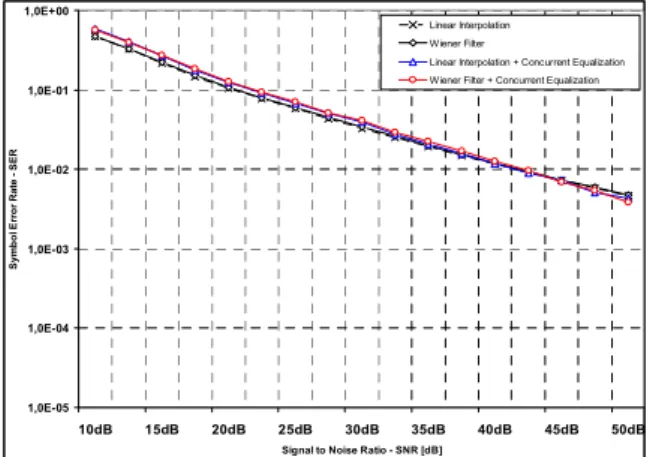
performance evaluation, we adopt the Brazil A-E channel multipath profiles [7] shown in Tables 2-5 with a channel bandwidth of 6 MHz. In order to evaluate the FDCCE performance under dynamic multipath, we apply Doppler rotation to the echo with highest amplitude level [10]. Since the purpose of the simulation is only to compare performances between channel estimation methods, it is assumed that there is no synchronization error.

Figures 5 to 10 show the SER curves versus the SNR for a ISDB-T receiver operating in the above conditions and with the receiver channel estimator implemented by using four distinct approaches – “Linear Interpolation”:

I i n

Y

_, is obtained by means of linear interpolation with no further update, i.e.,

Y

_nII_,i

=

Y

_nI_,i, using the grid specified in figure 3. “Wiener Filter”:

Y

_nI_,i is obtained by means of two cascaded time and frequency Wiener filters with no further update, i.e.,

Y

_nII_,i

=

Y

_nI_,i, using the grid specified in figure 3. The autocorrelation matrix [5] is of dimension 4×3, i.e., 4 taps for the frequency direction and 3 taps for the time direction. “Linear Interpolation + Concurrent Equalization”:

Y

_nI_,i is obtained by means of linear interpolation with further update

Y

_nII_,i obtained via FDCCE. “Wiener Filter + Concurrent Equalization”:

I i n

Y

_, is obtained by means of two cascaded time and frequency Wiener filters with further update

Y

_nII_,i obtained via FDCCE.

Table 2: “Brazil A” channel multipath profile.

Delay(µs) Amplitude(dB)

0.0 0.0 0.15 -13.8 2.22 -16.2 3.05 -14.9 5.86 -13.6 5.93 -16.4

Table 3: “Brazil B” channel multipath profile.

Delay(µs) Amplitude(dB)

0.0 0.0 0.3 -12.0 3.5 -4.0 4.4 -7.0 9.5 -15.0 12.7 -22.0

Table 4: “Brazil D” channel multipath profile.

Delay(µs) Amplitude(dB)

0.15 -0.1 0.63 -3.8 2.22 -2.6 3.05 -1.3 5.86 -0.0 5.93 -2.8

Table 5: “Brazil E” channel multipath profile.

1,0E-05 1,0E-04 1,0E-03 1,0E-02 1,0E-01 1,0E+00

10 15 20 25 30 35 40 45 50

Signal to Noise Ratio - SNR [dB]

S

y

mb

o

l E

rr

o

r R

a

te

- S

E

R

Linear Interpolation Wiener Filter

Linear Interpolation + Concurrent Equalization Wiener Filter + Concurrent Equalization

Figure 5: SER for the OFDM receiver operating under “Brazil A” channel multipath profile. Doppler frequency: 0 Hz.

1,0E-05 1,0E-04 1,0E-03 1,0E-02 1,0E-01 1,0E+00

10 15 20 25 30 35 40 45 50

Signal to Noise Ratio - SNR [dB]

Sy

m

b

o

l Err

o

r R

a

te

S

E

R

Linear Interpolation Wiener Filter

Linear Interpolation + Concurrent Equalization Wiener Filter + Concurrent Equalization

Figure 6: SER for the OFDM receiver operating under “Brazil A” channel multipath profile. Doppler frequency: 100 Hz.

1,0E-05 1,0E-04 1,0E-03 1,0E-02 1,0E-01 1,0E+00

10 15 20 25 30 35 40 45 50

Signal to Noise Ratio - SNR [dB]

Sy

m

b

o

l Er

ro

r R

a

te

SER

Linear Interpolation Wiener Filter

Linear Interpolation + Concurrent Equalization Wiener Filter + Concurrent Equalization

Figure 7: SER for the OFDM receiver operating under “Brazil B” channel multipath profile. Doppler frequency: 0 Hz.

1,0E-05 1,0E-04 1,0E-03 1,0E-02 1,0E-01 1,0E+00

10 15 20 25 30 35 40 45 50

Signal to Noise Ratio - SNR [dB]

Sy

m

b

o

l Er

ro

r R

a

te

SER

Linear Interpolation Wiener Filter

Linear Interpolation + Concurrent Equalization Wiener Filter + Concurrent Equalization

Figure 8: SER for the OFDM receiver operating under “Brazil B” channel multipath profile. Doppler frequency: 10 Hz.

1,0E-05 1,0E-04 1,0E-03 1,0E-02 1,0E-01 1,0E+00

10 15 20 25 30 35 40 45 50 Signal to Noise Ratio - SNR [dB]

S

y

m

b

o

l E

rr

o

r

R

a

te

- S

E

R

Linear Interpolation Wiener Filter

Linear Interpolation + Concurrent Equalization Wiener Filter + Concurrent Equalization

Figure 9: SER for the OFDM receiver operating under “Brazil D” channel multipath profile. Doppler frequency: 10 Hz.

1,0E-05 1,0E-04 1,0E-03 1,0E-02 1,0E-01 1,0E+00

10dB 15dB 20dB 25dB 30dB 35dB 40dB 45dB 50dB Signal to Noise Ratio - SNR [dB]

Sy

m

b

o

l Er

ro

r

R

a

te

SE

R

Linear Interpolation Wiener Filter

Linear Interpolation + Concurrent Equalization Wiener Filter + Concurrent Equalization

5.

C

ONCLUSION

The proposed Frequency Domain Concurrent Channel Equalizer (FDCCE) outperforms the classical channel estimation and compensation approaches for OFDM systems, such as Wiener interpolation and linear interpolation.

The adoption of the FDCCE after the linear interpolation procedure results in a lower symbol error rate when compared with the Wiener interpolator, while keeping the computational cost in a low level.

Actually, for a moderate multipath scenario such the Brazil A profile, and for a SNR above 27.5 dB, we obtained a zero symbol error rate, even when the mobile receiver is operating in an intense dynamic multipath scenario (Fdoppler = 100Hz).

6.

R

EFERENCES

[1] J. G. Proakis, Digital Communications, 3rd ed., McGraw-Hill, 1995.

[2] F. C. C. De Castro, M. C. F. De Castro and D. S. Arantes. "Concurrent Blind Deconvolution for Channel Equalization", IEEE International

Conference On Communications ICC2001, pp.

366-371, Helsinki, Finland, June 2001.

[3] S. Chen and E.S. Chang, “Fractionally spaced

blind equalization with low-complexity concurrent constant modulus algorithm and

soft decision-directed scheme”, International

Journal of Adaptive Control and Signal

Processing, 19(6) pp. 471-484, 2005.

[4] R. D. Gitling e S. B. Weinstein, “Fractionally-Spaced Equalization: An Improved Digital Transversal Equalizer”, Bell Systems Technical Journal, vol. 60, February 1981.

[5] F. Kazel and S. Kaiser, “Multi-Carrier and Spread Spectrum Systems”, John Wiley & Sons Ltd, The Atrium, Southern Gate, Chichester, West Sussex PO 19 8SQ, pp. 139-158, England, 2003.

[6] ARIB, “Transmission System for Digital Terrestrial Television Broadcasting”, STD-B31 Version 1.5, July 2003.

[7] Wu et.al. “An ATSC DTV Receiver With Improved Robustness to Multipath and Distributed Transmission Environments”, IEEE Transactions on Broadcasting, vol 50, no 1, pp. 32-41, March 2004.

[8] V. D. Nguyen, C. Hansen and H. P. Kuchenbecker, “Performance of channel estimation using pilot symbols for a coherent OFDM system”, WPMC’00 proceedings, pp. 842-847, Bangkok - Thailand November 2000.

[9] S. Haykin, Adaptative Filter Theory, 3rd ed., Prentice Hall, Upper Saddle River, New Jersey, 1996.

[10] M. Gosh, “Blind Decision Feedback