J. Braz. Comp. Soc. vol.12 número4

Design and FPGA Prototyping of a

H.264/AVC Main Profile

Decoder for HDTV

Luciano V. Agostini

, Arnaldo P. Azevedo Filho

, Wagston T. Staehler

, Vagner S. Rosa

,

Bruno Zatt

, Ana Cristina M. Pinto

, Roger Endrigo Porto

, Sergio Bampi

& Altamiro A. Susin

1

Informatics Institute

Federal University of Rio Grande do Sul Av. Bento Gonçalves, 9500, Campus do Vale, Bloco IV

Phone: +55 (51) 33089496

P.O.Box 15064, Zip 91501-970 - Porto Alegre - RS - BRAZIL {apafilho—tassoni—vsrosa—bzatt—cpinto—recporto—bampi}@inf.ufrgs.br

2

Informatics Department Federal University of Pelotas

Phone: +55 (53) 32757431

P.O.Box 354, Zip 96010-900 - Pelotas - RS - BRAZIL agostini@ufpel.edu.br

3

Electrical Engineering Department Federal University of Rio Grande do Sul

Av. Osvaldo Aranha, 103 Phone: +55 (51) 33083136

Zip 90035-190 - Porto Alegre – RS - BRAZIL altamiro.susin@ufrgs.br

Abstract

This paper presents the architecture, design, validation, and hardware prototyping of the main architectural blocks of main profile H.264/AVC decoder, namely the blocks: inverse transforms and quantization, intra prediction, motion compensation and deblocking filter, for a main profile H.264/AVC decoder. These architectures were designed to reach high throughputs and to be easily integrated with the other H.264/AVC modules. The architectures, all fully H.264/AVC compliant, were completely described in VHDL and further validated through simulations and

FPGA prototyping. They were prototyped using a Digilent XUP V2P board, containing a Virtex-II Pro XC2VP30 Xilinx FPGA. The post place-and-route synthesis results indicate that the designed architectures are able to process 114 million samples per second and, in the worst case, they are able to process 64 HDTV frames (1080x1920) per second, allowing their use in H.264/AVC decoders targeting real time HDTV applications.

1.

I

Video encoding techniques have been widely studied recently and implemented in hardware due to the increasing demand in this field. Digital TV, video exchange through internet, cell phones and PDAs as well as video streaming are examples of such applications that commonly require high quality and good compression rates.

The H.264/AVC (known as MPEG-4 part 10) [1] is the newest video coding standard which achieves significant improvements over the previous ones, in terms of compression rates [2]. H.264/AVC standard is organized in profiles (baseline, extended, main and high [1,3]), each one covering a set of applications. This work will focus the hardware for the main profile. The main profile is designed to achieve the highest efficiency in the encoding process for I (Intra), P (Predictive) and B (Bi-predictive) slices. This means that this profile covers applications that require the highest rates in compression and quality, such as HDTV.

This work was developed within the framework of an effort to develop intellectual property and to carry out an evaluation for the future Brazilian system of digital television, the SBTVD [4]. The H.264/AVC standard was chosen for the SBTVD source video coding, since it is currently the most advanced video compression standard. This paper focuses on the decoder design, which has to be massively produced for the end-user set. The main goal of this paper is to present a high throughput architecture developed by the authors for the H.264/AVC decoder from its architectural definition through prototyping. This design also targets an easy integration of the designed modules with the other H.264/AVC modules.

The prototype target is the FPGA. The decision to prototype in FPGA was due to the scope of the SBTVD project [4] which aimed at having a digital TV system prototyped in less than a year. Furthermore, considering the flexibility and the rapid prototyping characteristics of FPGAs, this technology is an excellent validation structure for complex digital designs, as is the case.

This paper is organized as follow. Section 2 presents an introduction to the H.264/AVC standard. Sections 3, 4, 5 and 6

present the architectures of the inverse transforms and quantization, the intra-prediction, the motion compensation module and the deblocking filter, respectively. Section 7 presents the architectures validation and section 8 presents the prototyping methodology. The synthesis results are presented in section 9. Finally, Section 10 presents the conclusions and future works.

2.

H.264/AVC

D

H.264/AVC standard defines four profiles: baseline, extended, high and main [1, 3]. The baseline was designed for low delay applications, as well as for applications that run on platforms with low power and in environment with high degree of packet losses. The extended profile focuses in streaming video applications. The high profile is divided in sub-profiles, all targeting high resolution videos. This work is focused in the hardware design of a H.264/AVC decoder, considering the main profile. The main profile differs from the baseline mainly by the inclusion of B slices, Weighted Prediction (WP), Interlaced video support and Context-based Adaptive Binary Arithmetic Coding (CABAC) [1, 3].

H.264/AVC decoder uses a structure similar with that used in the previous standards, but each module of a H.264/AVC decoder presents many innovations when compared with previous standards as MPEG-2 (also called H.262 [5]) or MPEG-4 part 2 [6]. Figure 1 shows the schematic of the decoder with its main modules. Input bit stream passes first through the entropy decoding. The next step is the inverse quantization and inverse transforms (Q-1 and T-1 modules in Figure 1) to recompose the prediction residues. INTER prediction (also called motion compensation - MC) reconstructs the macroblock (MB) from neighbor reference frames while INTRA prediction reconstructs the macroblock from the neighbor macroblocks in the same frame. INTER or INTRA prediction reconstructed macroblock is added to the residues and the results of this addition are sent to the deblocking filter. Finally, the reconstructed frame is filtered by deblocking filter and the result is sent to the frame memory.

Figure 1. H.264/AVC decoder diagram

MC

INTER Prediction Reference

Frames

Q-1

+ T-1

Current Frame

(reconstructed)

Entropy Decoder INTRA

Prediction

Filter Compressed Video

Stream Input Video

H.264/AVC entropy coding uses three main tools to allow a high data compression: Exp-Golomb coding, Context Adaptive Variable Length Coding (CAVLC) and Context Adaptive Binary Arithmetic Coding (CABAC) [3]. The main innovation of the entropy coding is the use of a context adaptive coding. In this case, the coding process depends on the element that will be coded, on the coding algorithm phase, and on the previously coded elements. Entropy coding process defines that the residual information (quantized coefficients) is entropy coded using CAVLC or CABAC, while the other coding units are coded using Exp-Golomb codes [3].

Q-1

and T-1

modules are responsible to generate the residual data that are added to the prediction results to produce the reconstructed frame. Inverse quantization module performs a scalar multiplication. The quantization value is defined by the QP external parameter [3]. There are three main innovations in the transforms of this standard. The first one is related with the block dimensions which were defined as 4x4, instead of the traditional 8x8 block size. The second one is related with the use of three different two dimensional transforms, depending on the type of input data. These transforms are 4x4 inverse discrete cosines transform, 4x4 inverse Hadamard transform and 2x2 inverse Hadamard transform [3]. The third one is the use of an integer approximation of these transforms, to allow a fixed point hardware implementation. The inverse transforms operations are divided in two parts, one is applied before and other is applied after the inverse quantization. First the inverse Hadamard is applied (when used), then the inverse quantization is applied and, finally, the inverse DCT is applied.

The motion compensation (MC) operation can be regarded as a copying of the predicted macroblock from the reference frame, and then to add the predicted MB with the residual MB to reconstruct the MB in current frame. This is the most demanding component of the H.264/AVC decoder, consuming more than a half of the complete computation power used with the decoding process [2]. Most of the H.264/AVC innovations rely on the motion compensation process. An important feature of this module is the use of blocks with variable sizes (16x16, 16x8, 8x16, 8x8, 8x4, 4x8 or 4x4). Other important feature is the use of a quarter-sample accuracy which is used to define the best matching and to reconstruct the frame. H.264/AVC also allows the use of multiple reference frames, which can be past or future frames in the temporal order. Bi-predictive, weighted and direct predictions are also innovations of this standard. Other feature is related to the motion vectors that can point to positions outside the frame. Finally, the motion vector prediction is an important innovation, once these vectors are predicted from the neighbor motion vectors [3].

H.264/AVC defines an Intra prediction process in the spatial domain [3] and this is an innovation. The macroblocks of the current frame can be predicted considering the previously processed macroblocks of the same frame. Intra

prediction can process blocks with 16x16, 4x4 (considering luma information) or 8x8 (considering chroma information). There are nine different prediction modes for 4x4 luma blocks, four modes for 16x16 luma modules and four modes for 8x8 chroma blocks [3].

H.264/AVC standardizes the use of a deblocking filter (also called loop filter). This is an important improvement added to this standard, since this filter was optional in the previous standards. The most important characteristic of this filter is that it is context adaptive and it is able to distinguish a real image border from an artifact generated when the quantization step has a high value. The boundary strength (BS) defines the filtering strength and it can take five different values from 0 (no filtering) to 4 (strongest filtering) [3].

3.

I

T

Q

A

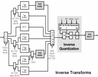
The designed architecture for the Q-1 and T-1 modules is generically presented in Figure 2. It is important to notice the presence of the inverse quantization module between the operations of T-1 module.

As discussed before, the main goal of this design was to reach a high throughput hardware solution in order to support HDTV. This architecture uses a balanced pipeline and it processes one sample per cycle. This constant production rate depends neither on the input data color type nor on the prediction mode used to generate the inputs. Finally, the input bit width is parameterizable to facilitate the integration.

The inverse transforms module uses three different two dimensional transforms, according to the type of input data. These transforms are: 4x4 inverse discrete cosine transform, 4x4 inverse Hadamard transform and 2x2 inverse Hadamard transform [1,7]. The inverse transforms were designed to perform the two dimensional calculations without using the separability property. Then, the first step to design them was to decompose their mathematical definition [7] in algorithms that do not use the separability property [8]. The architectures designed for the inverse transforms use only one operator at each pipeline stage to save hardware resources. The architectures of the 2-D IDCT and of the 4x4 2-D inverse Hadamard were designed in a pipeline with 4 stages, with 64 cycles of latency [8]. The 2-D inverse Hadamard was designed in a pipeline with 2 stages, with 8 cycles of latency. All T-1

datapaths have the same 133 cycles of latency.

In the inverse quantization architecture, all the internal constants had been previously calculated and stored in memory, saving computation time and logic cells of the target FPGA. The designed architecture is composed by a constants generator (tables stored in memory), a multiplier, an adder and a barrel shifter.

transforms and quantization architecture to guarantee the desired architectural synchronism. Buffers and FIFO were designed using registers instead of regular memory.

Figure 2. T-1

and Q-1

module diagram

There are a few papers that present dedicated hardware designs for H.264/AVC transforms and quantization. The solutions proposed in [9, 10, 11, 12] are multitransform architectures that are able to process the calculations related to the four 4x4 forward and inverse transforms. Our design solution [9] processes also the 2x2 forward and inverse Hadamards and this solution is able to select the level of parallelism desired in the computations. The designs presented in [13] grouped individually each 4x4 transform with their specific quantization, but they do not group a complete inverse transforms and quantization module.

The number of samples processed in each clock cycle varies from 4 to 16 in designs found in the literature. This parallelism allows a very high processing rate that surpasses the requirements of high resolution applications. This very high performance, however, implies several difficulties to use these architectures in a complete inverse transforms and quantization architecture required in a H.264/AVC decoder. In this case, the memory overhead will be an important challenge to be solved. Also, the connection of these modules with the remaining ones will heavily use routing resources. Finally, it is really very complex to design parallel H.264/AVC entropy decoder and inter or intra prediction modules with the necessary throughput required by the parallel transforms. For these reasons and to reduce the use of hardware resources, we decided to design an architecture to reach the HDTV performance requirements processing just one sample per clock cycle.

4.

I

P

A

One of the innovations brought by the H.264/AVC is that

no macroblock (MB) is coded without the associated prediction including the MBs from I slices. Thus, the transforms are always applied in a prediction error [3].

The Intra prediction is based in the value of the pixels above and to the left of a block or MB. For the luma, the Intra prediction is performed for blocks with 4x4 or 16x16 samples. The H.264/AVC allows the use of nine modes of prediction for 4x4 blocks (luma4x4) and four different prediction modes for 16x16 blocks (luma16x16). The four modes of prediction for 8x8 blocks of chroma (chroma8x8) are equivalent to luma16x16. The different modes allow the prediction of soft areas as well as the edges [14].

The inputs of the Intra prediction are the samples reconstructed before the filter and the type of code of each MB inside the picture [1]. The outputs are the predicted samples to be added to the residue of the inverse transform.

The Intra prediction architecture and implementation was divided in three parts, as can be seen at Figure 3: NSB (Neighboring Samples Buffer); SED (Syntactic Elements Decoder); and PSP (Predict Samples Processor).

Figure 3. Block diagram of Intra prediction architecture

NSB module stores the neighboring samples that will be used to predict the subsequent macroblocks. SED module decodes the syntactic elements supplied for the control of the predictor. PSP module uses the information provided by other parts and processes the predicted samples. This architecture produces four predicted samples each cycle in a fixed order. PSP has 4 cycles of latency to process 4 samples.

No similar work compared to this designed architecture was presented in the literature for the Intra frame prediction, since it was developed targeting a H.264/AVC decoder for FPGA prototyping. A previous work of our team [15] was published and presented the first results of this design.

4.1. NEIGHBORING SAMPLES BUFFER (NSB)

NSB knows the position of each sample since the decoding order was previously established. Other than buffering, the NSB is responsible for making all the neighbors of a prediction available in a parallel form.

4.2. SYNTACTIC ELEMENTS DECODER (SED)

This part of the Intra predictor architecture receives all the syntactic elements and decodes data that will be supplied to control the PSP. These data are:

Prediction Type: it informs the codification type which can be luma16x16, luma4x4 or chroma8x8.

Prediction Mode: when the prediction type is luma16x16 or chroma8x8, the prediction mode is generated directly from a syntactic element. When the prediction type is luma4x4 each of the sixteen 4x4 blocks of a MB have their own mode that is predicted based on the neighbor blocks modes.

Availability of the neighboring sample: it informs if the neighbor samples are available. This information relies on the MB position on the frame.

4.3. PREDICT SAMPLES PROCESSOR (PSP)

This part of the architecture uses the information supplied by the NSB and the SED to calculate the predicted samples. Four samples per cycle are produced by this module. The implementation was divided in three parts: calculation of the modes luma4x4, plane mode calculation, and other luma16x16 and chroma modes calculation. Each part was implemented as a separate architecture.

The 4x4 luma prediction macroblocks are subdivided in sixteen 4x4 blocks, and each of them are predicted independently. The 4x4 prediction is better than 16x16 prediction once it achieves more accurate results for heterogeneous regions of an image. This part of the system needs to perform nine modes of prediction, depending on the mode received from control and neighbors that are available. The engine processes 13 neighbors (4 on the left, 8 above and 1 on top-left corner) and sends out 16 sample predictions.

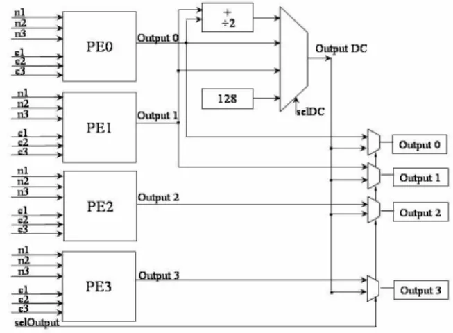
Figure 4 presents an approach that has four processing element (PE) which can process 4 samples per cycle. All PEs are identical because every pixel in every mode can be calculated as presented in (1) (DC mode is the exception):

Pi = (n1 + c1 × n2 + n3 + c2) >> c3 (1)

Depending on the chosen mode, the values of n1, n2, n3, c1, c2 and c3 are switched.

In order to process DC mode, processing elements PE0 and PE1 are used jointly. Additional hardware is necessary to add results, to divide by 2 and to select the DC output according to the availability of upper and left neighbors.

Figure 4. Luma4x4 module diagram for the PSP.

Plane mode can be used for luma16x16 prediction and for chroma prediction as well. The hardware architecture is subdivided in two parts. The first is responsible for calculating constants “a”, “b” and “c” by using neighboring samples, and it was implemented as three stage pipeline. The second part utilizes these constants for calculating the predicted samples. This implementation also has a rate of four samples per cycle. It needs just one control signal, which is the position of samples that are being produced.

There is also a DC mode for luma16x16 and for chroma samples. Its output is the mean of all neighboring samples available. For every pixel in a macroblock the output is the same value, i.e. the DC value. This implementation consists in adders and a multiplexer that chooses the correct output depending on availability of neighboring samples.

5.

M

C

A

In order to increase coding efficiency, the H.264/AVC adopted a number of new technical developments, such as variable block-size; multiple reference pictures; quarter-sample accuracy; weighted prediction; bi-prediction and direct prediction. Most of these new developments rely on the motion compensation process [2]. Thus, this module is the most demanding component of the decoder, consuming more than half of its computation time [16].

Motion compensation operation is, basically, to copy the predicted MB from the reference frame, adding this predicted MB to the residual MB. Thus, this operation allows the reconstruction of the MB in the current frame.

The decoded frames used as reference are stored in an external memory. The area for the motion compensation is read from this external memory. The problem here is that the area, and sometimes the reference frame, is known just after the motion vectors prediction, making this process longer.

The sample processing is formed by the quarter-sample interpolation, weighted prediction and clipping. The bi-predictive motion compensation is also supported by the developed architecture.

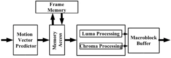
The proposed architecture was designed in a hierarchical pipeline formed by: Motion Vector Predictor, Memory Access and Sample Processing. Figure 5 shows the datapath of the proposed motion compensation module.

Luma Processing

Chroma Processing

Macroblock Buffer Motion

Vector Predictor _Mem

o

ry

A

cc

es

s

Frame Memory

Figure 5. Motion Compensation (MC) datapath.

5.1. MOTION VECTOR PREDICTOR

The Motion Vector Predictor (MVPr) function restores the motion vectors and reference frames needed in the interpolation process. The predictor inputs are differential motion vectors and reference frames, besides the slice and macroblock information. For bi-predictive blocks, the direct prediction mode can be set, using information from spatial or temporal neighbor blocks.

MVPr architecture was modeled as a set of registers and a state machine, for a highly sequential algorithm implementation. Ten sets of registers were used to store the neighbor blocks information. This predictor calculates list 0 as well as list 1 (two lists of previously decoded frames which are used in the prediction process [1,3]) of motion vectors and reference frames in parallel. Internal memory stores information of the collocated frame used in direct prediction. The state machine has 45 states and it supports the vector prediction for non interlaced videos in main profile.

Motion Vector Predictor has a minimal latency of 20 cycles but it takes, in average, 123.5 cycles to process each macroblock when a video with an IPBBP frame sequence is processed.

5.2. MEMORY ACCESS

Due to filter window size, some reference areas are used many times to reconstruct image blocks, and every time these areas must come from the memory to the MC interpolator. The retransmission of this redundant data uses large amount of memory bandwidth. To reduce the memory bandwidth, a memory hierarchy was designed.

After a careful balancing study of miss ratio, hardware resources used and latency to copy data from memory to cache, a 32 sets three-dimensional cache memory was proposed using 16 lines X 40 rows cache sets. The cache output provides to the sample processing, at the same time, one line of luma and two lines of chroma samples.

The policy used in substitution mechanism was FIFO. This policy was chosen because it requires less hardware resources to be implemented than other policies and this policy presented good results.

In case of a cache miss, a state machine requests these data to the external memory. The external memory sends 40 luma lines and 32 chroma lines to be stored in cache. This process is controlled by a handshake mechanism. After the first 16 luma lines had been written in cache, the cache can start a new reading cycle.

Some techniques to save memory access were adapted from [17] and used in this design:

Reading only necessary samples: There are cases where just a part of the interpolation window is used. In these cases, the rest of the interpolation window does not need to be read from external memory.

Interleaved Y, Cb, and Cr samples: Interleaving Y, Cb and Cr samples in the same external memory area reduces the memory bandwidth, saving extra clock cycles for memory line swap.

The cache memory combined with the memory bandwidth saving techniques proposed in [17], reduced the memory access up to 60% for the tested cases. When one cycle penalty for changing the memory line is necessary, 75% or more in access cycles to an external memory are saved.

5.3. SAMPLE PROCESSING

As presented in Figure 5, the luma and chroma samples processing works in parallel. Some preliminary results of this architecture were presented in [1,8]. There are one luma and one chroma datapaths for motion compensation of the blocks. A 384 position buffer stores the results of one luma and two chroma macroblocks and synchronizes the MC module to other decoder components.

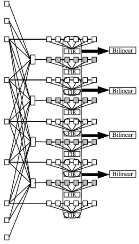
Figure 6. Luma sample processing datapath.

The luma interpolator is presented in Figure 7 and it decomposes the 2-D FIR filter in two 1-D FIR filters (one vertical and other horizontal). This approach is based on [19]. Four vertical and nine horizontal 6-tap FIR filters (1, -5, 20, -5, 1) generate the half-sample interpolation while four bilinear interpolators generate the quarter-sample interpolation results.

Figure 7. Luma interpolator architecture

Luma datapath is four samples wide and each chroma datapath is two samples wide. This strategy is required to meet the throughput for HDTV decoding.

To handle bi-predictive prediction slices without duplicating the interpolators and the WP datapaths, the architecture process one block from each list serially. Both reference image areas are loaded in the input buffer. The list 0 reference area is processed and its results are saved in a buffer (4x4 for luma and 2x2 for chroma samples). When WP generates the valid interpolated results from list 1, these results are sent to the average calculation. The list 0 results that are stored in the buffer are also sent to the average calculation. The average of these two results is then calculated and this value is sent to the clipping calculation.

In the current literature, a motion compensation architecture with support for bi-prediction is not available. Some comparisons with other works are possible based on other prediction modules.

In [19] a H.264/AVC baseline motion compensation is described. Our work uses the architectural idea of the luma interpolator presented in [19]. However, adaptations were made to allow the bi-predictive support and the duplication of performance. Other works [20, 21] focus specifically on the interpolation problem and they do not present solutions for bi-predictive processing.

6.

D

F

A

The Deblocking Filtering process consists of possibly modifying pixels at the four block edges by an adaptive filtering process. The filtering process is performed by one of the five different standardized filters, selected by mean of boundary strength (BS) calculation. This boundary strength is obtained from the block type and some pixel arithmetic to verify if the existing pixel differences along the border are a natural border or an artifact [3]. Figure 8(a) presents some definitions employed in the deblocking filter. From this figure, note that a block has 4x4 pixels samples; the border is the interface between two neighbor blocks; a line-of-pixel is four samples (luma or chroma pixel components) from the same block orthogonal to the border; the current block (Q) is the block being processed, while the previous block (P) is the block already processed (left or top neighbor). The filter operation can modify pixels in both the previous and the current blocks. The filters employed in the deblocking filter are one-dimensional. The two dimensional behavior is obtained by applying the filter on both vertical and horizontal edges of all 4x4 luma or chroma blocks, as illustrated in Figure 8(b).

p 3 p 2 p 1 p 0 q 0 q 1 q 2 q 3 p 3 p 2 p 1 p 0 q 0 q 1 q 2 q 3 p 3 p 2 p 1 p 0 q 0 q 1 q 2 q 3 p 3 p 2 p 1 p 0 q 0 q 1 q 2 q 3 P r e v ie w s B lo c k ( P ) C u r r e n t B lo c k ( Q )

S a m p le ( Y , C b , o r C r ) B o r d e r L O P

p 3 p 2 p 1 p 0 q 0 q 1 q 2 q 3 p 3 p 2 p 1 p 0 q 0 q 1 q 2 q 3 p 3 p 2 p 1 p 0 q 0 q 1 q 2 q 3 p 3 p 2 p 1 p 0 q 0 q 1 q 2 q 3 P r e v ie w s B lo c k ( P ) C u r r e n t B lo c k ( Q )

S a m p le ( Y , C b , o r C r ) B o r d e r L O P

(a)

P Q

Phase 1

P Q

Phase 2

P

Q Phase 3

P

Q Phase 4

P Q

Phase 1

P Q

Phase 2

P

Q Phase 3

P

Q Phase 4

(b)

Deblocking filter input are pixel data and block context information from previews blocks of the decoder and output are filtered pixel data according to the standard.

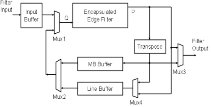
The edge filter is implemented as a 16 stage pipeline containing both the decision logic and the filters. It operates for both vertical and horizontal edges of the blocks. Due to a block reordering in the input buffer, it is possible to connect the Q output to the P input of the edge filter. The encapsulated filter contains the edge filter and the additional buffers for that feedback loop.

Figure 9 shows the block diagram of the proposed deblocking filter architecture and the next paragraphs present a quick description of each module from this figure.

Figure 9. Deblocking filter block diagram

Input Buffer: pixel data are fed into the filter through the input buffer. Data arrives organized in double Z for luma followed by Cb and Cr blocks and is read in columns for the deblocking processing. For this reason, an input buffer is needed and must be filled with at least one complete MB (luma and chroma) to start the filtering process.

Edge Filter: it is responsible for all filter functionality, including the thresholds and BS calculation and filtering itself. A 16 stage pipeline was used due to data dependencies.

Edge Filter Encapsulation: this block encapsulates the edge filter connecting the Q output to the P input and implements some additional buffers to data control.

MB Buffer: The MB buffer stores two different types of blocks. First, the right block column from the left macroblock for use in the external vertical border filtering process. And the vertically filtered blocks transposed and reordered for the horizontal edge filtering. A total of 32 blocks and its decoding information are stored in the MB Buffer. This buffer was implemented as a dual-port RAM and therefore it can be read or written when necessary (dual-port RAMs are available as building blocks in the target FPGA).

Line Buffer: The line buffer stores the blocks needed to make the external horizontal border filtering in the next MB line. In order to perform this task, eight blocks, from the upper MB, are needed. It is also needed all decoding information

related to these eight blocks. The necessary memory in the line buffer depends on the maximum image width required to filter.

Transpose: In this part of the filter, data from a 4x4 pixel block are transposed. The transpose was implemented using two blocks of memory. So, the required data can be read at the same cycle of the new arriving one.

This 16-stage pipeline architecture perform one luma and two chroma macroblocks at each 256 clock cycles leading to a production rate of 1.5 samples per clock cycle, or 1 pixel per clock cycle (considering the 4:2:0 color relation). No other implementation was found targeting FPGA, making comparison from this work to others published somewhat difficult. Therefore, [22] and [23] presents some ASIC implementations and comparisons tables. Even for ASIC implementations, no other 16-stage pipeline was found, making this implementation completely unique.

7.

V

P

To validate the architectures that were developed an exhaustive simulation approach was chosen. This approach requires a large number of test cases, so that additional functions were inserted in the H.264/AVC reference software. Real video sequences were processed by the H.264/AVC reference software to generate the needed data for each module validation. This data was then stored in text files with a predefined format.

The Mentor Graphics ModelSim tool [24] was used to run the simulations necessary for the validation of all designs. Testbenchs were described in VHDL to manage the input and output architecture data. The input stimuli were the data extracted from the reference software. Its output results were saved in different text files. The comparison of the proposed architecture results and reference software results was performed by specific software developed to validate the proposed architecture. These steps were repeated exhaustively for some coded video sequences with the main profile tools on.

The first validation step consists of a behavioral model simulation of the designed architectures. The second step repeats the validation process considering a post and-route model of these architectures. To generate the post place-and-route model the RTL VHDL description was synthesized to the target FPGA device. The synthesis result is a back annotated VHDL mapped to the FPGA device structure, with delays of cells and wires. In this step the Xilinx ISE tool [25] was used with the ModelSim in order to generate the post place-and-route information about the architectures. The target device selected was a Xilinx XC2VP30 Virtex-II Pro FPGA [26].

produced by the reference software. After VHDL debugging process, the comparison did not point any differences between the models. Then, the architecture was considered validated in accordance with the H.264/AVC Main Profile standard.

8.

D

M

P

The prototyping was done using the XUP-V2P development board [27] designed by Digilent Inc. This board has a XC2VP30 Virtex-II Pro FPGA (with two PowerPC 405 processors hardwired) [26], serial port, VGA output and many other interface resources [27]. It was also fitted with a DDR SDRAM DIMM module of 512MB.

Xilinx EDK [28] was used to create the entire programming platform which is needed for the prototyping process. Each designed architecture module was connected to the processor bus and prototyped individually. One of the PowerPC processors was employed as a controller for the prototyped module, emulating the other modules of the decoder. The input stimuli were sent to the prototyping system through a RS-232 serial port, using a terminal program running in a host PC. The processor sends the stimuli to the architectures and the module results are sent back to the host PC by the processor. The results of the prototyped module are compared to the reference software results, indicating if the prototyped architecture was properly running on the target device. This comparison was made in the host PC after the module finishes its calculations.

The validation process of the prototype started with a functional verification. A PowerPC processor system was synthesized with the module under validation (MUV) and the MUV stimuli, including the clock signal, were generated by the processor system and send through the processor system bus. The outputs from the MUV are sampled directly by the processor system bus. As the clock for the MUV is generated by software in this approach, the processor system could be arbitrarily slow. Figure 10 illustrates this prototyping approach.

This functional verification worked correctly, but the critical paths of the MUV could not be exercised on the FPGA using this approach, due to the slow clock applied.

Figure 10. Functional prototype validation aproach.

Another prototyping approach will be employed to validate the MUV at full speed. In this approach the stimuli will be sent from the processor system at arbitrary speeds and

accumulated in an input stimulus buffer. This buffer will store enough stimuli for one burst cycle. When the buffer is full, the buffered stimuli will be sent to the MUV and, at the same time, the block output buffer will be filled with the data produced by the MUV. These bursts of stimuli will be sent to the MUV at a full clock speed, making the full speed prototype validation possible.

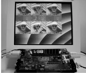
In some modules (intra prediction, motion compensation and deblocking filter), a VGA frame buffer was synthesized and some visual results could be sent directly from the prototyping board to a video display. Figure 11 presents an example of a video output from the Motion Compensation prototype.

The next development step is the integration of the modules. The latencies of all modules were previously defined to facilitate the integration process. The three main datapaths of the decoder, as presented in Figure 1 are (1) motion compensation, (2) intra prediction and (3) the group formed by entropy decoder, inverse transforms and inverse quantization. These main datapaths present the same latency to allow a rapid synchronization of the decoder. The same approach employed for prototype verification of individual decoder modules was employed to verify the integrated modules. Currently, intra prediction, T-1

, Q-1

and the deblocking filter modules are already integrated and motion compensation module is being integrated.

Figure 11. Motion Compensation prototyping.

9.

S

R

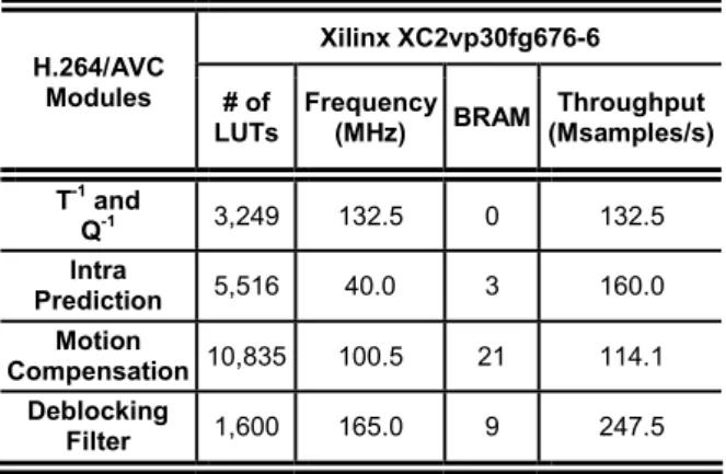
Table 1. H.264/AVC Decoder Synthesis Results

Xilinx XC2vp30fg676-6 H.264/AVC

Modules _{# of} LUTs

Frequency (MHz) BRAM

Throughput (Msamples/s)

T-1 _and

Q-1 3,249 132.5 0 132.5

Intra

Prediction 5,516 40.0 3 160.0

Motion

Compensation 10,835 100.5 21 114.1

Deblocking

Filter 1,600 165.0 9 247.5

The post place-and-route synthesis results indicate that the designed architectures are able to process more than 110 million samples per second and, in the worst case, they are able to process 36.7 HDTV frames per second, allowing their use in H.264/AVC decoders targeting real time HDTV applications. Considering a HDTV frame with 1080 x 1920 pixels at 30 fps and considering a downsampling ratio of 4:2:0 [3], then the required throughput is at least 93.3 million samples per second.

Inverse transforms and quantization synthesis indicated that this module is able to run at 132.5MHz, reaching a processing rate of 132.5 million samples per second, once this architecture was designed to produce one sample per cycle. This solution is able to process 42.6 HDTV frames per second, surpassing the requirements for real time in this resolution. The inverse transforms and quantization architecture uses 3,249 LUTs of the device. This high use of resources is mainly caused by the buffers (designed as registers) which are used to synchronize the internal operations.

Intra prediction synthesis indicated a maximum operating frequency of 40MHz. This is due to the high complexity of the data flow inside the module. Indeed, it is able to process four input samples per cycle, so the throughput is 160 million samples per second, far above the required throughput and allowing it to process 51.5 HDTV frames per second.

Motion compensation synthesis consumes 8,465 slices, 5,671 registers, 10,835 LUTs, 21 internal memory modules and 12 multipliers of the target FPGA. The minimum latency achieved is 233 cycles to process one macroblock, and the maximum is 590, without cache misses. The maximum frequency is 100.5 MHz. The architecture proposed is able to process 36.7 totally bi-predictive HDTV frames per second, in the worst case. Processing P frames only, this rate increases to 64.3 frames per second, since it does not use bi-prediction.

Deblocking filter architecture was designed around a pipelined edge filter. The filter requires eight samples for the processing. So, the filter architecture was designed to be four

samples wide. Due to data dependencies as well as the fact that the samples need to go through the edge filter twice (for vertical and horizontal filtering), the processing rate of the deblocking filter is 1.5 samples per clock cycle. Achieving a frequency of 165 MHz, the architecture is able to process up to 247.5 million samples per second, allowing the filter to process 79.6 HDTV frames per second, exceeding the HDTV requirements.

The initial integration shows no significant performance degradation when all modules are mapped together, since the modules were designed with interfaces that match timing and data format at each block. Furthermore, the target FPGA is large enough to integrate the modules, leading no place-and-route bottlenecks.

Almost all the designs related to the H.264/AVC standard reported in the literature are directed to standard-cells technology and the work presented in this paper has been targeted to FPGAs. Thus, comparisons of performance and resources usage between those solutions and the one described here are not meaningful.

10.

C

This paper presented the design, validation, and prototyping of architectures for a main profile H.264/AVC decoder. The decoder modules were designed to meet HDTV (1920x1080 at 30fps) requirements as well as to be easily integrated with other modules. These architectures were targeted to FPGAs, employing all types of resources available in the target device, like memory, multipliers and processors.

This work was focused on FPGA implementation, but the VHDL code itself was developed as portable as possible. A FPGA to ASIC migration should be straightforward, although some architectural modifications would be necessary to optimize the design to a given ASIC technology.

The synthesis results indicate that the designed architectures are able to process at least 114 million samples per second, surpassing the HDTV requirement of 93 million samples per second at a 4:2:0 color ratio. The designed architectures reach, in the worst case, the processing of 36.7 HDTV frames per second, allowing their use in H.264/AVC decoders for HDTV.

11.

R

[1] Video Coding Experts Group. Advanced video coding for generic audiovisual services. ITU-T Recommendation H.264, International Telecommunication Union, Mar 2005.

[2] G. Sullivan, T. Wiegand. Video compression – from concepts to the H.264/AVC standard. Proceeding of the IEEE, 93(1):18-31, 2005.

[3] I. Richardson. H.264 and MPEG–4 video compression: Video coding for next–generation multimedia. John Wiley & Sons, Chichester, 2003.

[4] Brazilian Communication Ministry. Brazilian digital TV system. http://sbtvd.cpqd.com.br, Mar. 2007.

[5] Video Coding Experts Group. Generic coding of moving pictures and associated audio information – Part 2: Video. ITU-T Recommendation H.262, International Telecommunication Union, 1994.

[6] Motion Picture Experts Group. MPEG-4 Part 2: Coding of audio visual objects – Part 2: Visual. ISO/IEC Recommendation 14496-2, International Organization for Standardization, 1999.

[7] H. Malvar, A. Hallapuro, M. Karczewicz, L. Kerofsky. Low–complexity transform and quantization in H.264/AVC. IEEE Transactions on Circuits and Systems for Video Technology, 13(7):598–603, 2003.

[8] L. Agostini, M. Porto, J. Güntzel, R. Porto, S. Bampi. High throughput FPGA based architecture for H.264/AVC inverse transforms and quantization. In Proceedings of IEEE International Midwest Symposium on Circuits and Systems, San Juan, 2006.

[9] L. Agostini, R. Porto, J. Güntzel, I. Silva, S. Bampi High throughput multitransform and multiparallelism IP directed to the H.264/AVC video compression standard. In Proceedings of IEEE International Symposium on Circuits and Systems, Kós, pages 5419-5422, 2006.

[10] T. Wang, Y. Huang, H. Fang; L. Chen. Parallel 4x4 2D transform and inverse transform architecture for MPEG-4 AVC/H.264. In Proceedings of IEEE International Symposium on Circuits and Systems, Bangkok, pages 800-803, 2003.

[11] Z. Cheng, C. Chen, B. Liu, J. Yang. High throughput 2-D transform architectures for H.264 advanced video coders. In Proceedings of IEEE

Asia-Pacific Conference on Circuits and Systems, Singapore, pages 1141-1144, 2004.

[12] K. Chen, J. Guo, J. Wang. An efficient direct 2-D transform coding IP design for MPEG-4 AVC/H.264. In Proceedings of IEEE International Symposium on Circuits and Systems, Kobe, pages 4517-4520, 2005.

[13] H. Lin, Y. Chao, C. Chen, B. Liu, J. Yang. Combined 2-D transform and quantization architectures for H.264 video coders. In Proceedings of IEEE International Symposium on Circuits and Systems, Kobe, pages 1802-1805, 2005.

[14] Y. Huang, B. Hsieh. Analysis, fast algorithm, and VLSI architecture design for H.264/AVC intra frame coder. IEEE Transactions on Circuits and System for Video Technology, 15(3): 378-401, 2005.

[15] W. Staehler, E. Berriel, A. Susin, S. Bampi. Architecture of an HDTV intraframe predictor for an H.264 decoder. In Proceedings of IFIP International Conference on Very Large Scale Integration, Perth, pages 228-233, 2006.

[16] X. Zhou, E. Li, Y. Chen. Implementation of H.264 decoder on general-purpose processors with media instructions. In Proceedings of SPIE Conference on Image and Video Communications and Processing, Santa Clara, pages 224-235, 2003.

[17] R. Wang, J. Li; C. Huang. Motion compensation memory access optimization strategies for H.264/AVC decoder. In Proceedings of IEEE International Conference on Acoustics, Speech, and Signal Processing, Philadelphia, volume 5, pages 97-100, 2005.

[18] A. Azevedo, B. Zatt, L. Agostini, S. Bampi. Motion compensation decoder architecture for H.264/AVC main profile targeting HDTV. In Proceedings of IFIP International Conference on Very Large Scale Integration, Perth, pages 52-57, 2006.

[19] S. Wang, T. Lin; T. Liu; C. Lee. A new motion compensation design for H.264/AVC decoder. In Proceedings of IEEE International Symposium on Circuits and Systems, Kobe, pages 4558-4561, 2005.

[21] W. Lie, H. Yeh; T. Lin, C. Chen. Hardware efficient computing architecture for motion compensation interpolation in H.264 video coding. In Proceedings of IEEE International Symposium on Circuits and Systems, Kobe, pages 2136-2139, 2005.

[22] H. Lin, J. Yang, B. Liu, J. Yang. Efficient deblocking filter architecture for H.264 video coders. In Proceedings of IEEE International Symposium on Circuits and Systems, Kós, pages 2617-2620, 2006.

[23] G. Khurana, A. Kassim, T. Chua, M. Mi. A pipelined hardware implementation of in-loop deblocking filter in H.264/AVC. IEEE Transactions on Consumer Electronics, 52(2):536-540, 2006.

[24] Mentor Graphics Corporation. ModelSim SE User’s Manual - Software Version 6.2d. http://www.model.com/resources/resources_manu als.asp, Mar. 2007.

[25] Xilinx Inc. Xilinx ISE 8.2i software manuals and help. http://www.xilinx.com/support/sw_manuals/ xilinx82/index.htm, Mar. 2007.

[26] Xilinx Inc. Virtex-II Pro and Virtex-II Pro X platform FPGAs: complete data sheet. http://direct.xilinx.com/bvdocs/publications/ds083 .pdf, Mar. 2007.

[27] Xilinx Inc. Xilinx university program Virtex-II Pro development system - hardware reference

manual. http://direct.xilinx.com/bvdocs/ userguides/ug069.pdf, Mar. 2007.

[28] Xilinx Inc. Embedded system tools reference manual - embedded development Kit, EDK 8.2i. http://www.xilinx.com/ise/embedded/est_rm.pdf, Mar. 2007.