38
1
Handbook of Optimiza
tion
INTELLIGENT SYSTEMS REFERENCE LIBRARY
Volume 38
Handbook of Optimization
ISBN 978-3-642-30503-0
The aim of this series is to publish a Reference Library, including novel advances and developments in all aspects of Intelligent Systems in an easily accessible and well structured form. The series includes reference works, handbooks, compendia, textbooks, well-structured monographs, dictionaries, and encyclopedias. It contains well integrated knowledge and current information in the fi eld of Intelligent Systems. The series covers the theory, applications, and design methods of Intelligent Systems. Virtually all disciplines such as engineering, computer science, avionics, business, e-commerce, environment, healthcare, physics and life science are included.
Optimization problems were and still are the focus of mathematics from antiquity to the present. Since the beginning of our civilization, the human race has had to confront numerous technological challenges, such as fi nding the optimal solution of various problems including control technologies, power sources construction, applications in economy, mechanical engineering and energy distribution amongst others. These examples encompass both ancient as well as modern technologies like the fi rst electrical energy distribution network in USA etc. Some of the key principles formulated in the middle ages were done by Johannes Kepler (Problem of the wine barrels), Johan Bernoulli (brachystochrone problem), Leonhard Euler (Calculus of Variations), Lagrange (Principle multipliers), that were formulated primarily in the ancient world and are of a geometric nature. In the beginning of the modern era, works of L.V. Kantorovich and G.B. Dantzig (so-called linear programming) can be considered amongst others. This book discusses a wide spectrum of optimization methods from classical to modern, alike heuristics. Novel as well as classical techniques is also discussed in this book, including its mutual intersection. Together with many interesting chapters, a reader will also encounter various methods used for proposed optimization approaches, such as game theory and evolutionary algorithms or modelling of evolutionary algorithm dynamics like complex networks.
INTELLIGENT SYSTEMS REFERENCE LIBRARY
Volume 38
Handbook of
Optimization
123
Ivan Zelinka
Vaclav Snasel
Ajith Abraham (Eds.)
Zelinka • Snasel
Abraham
(E
ds.)
Ivan Zelinka • Vaclav Snasel • Ajith Abraham (Eds.)
From Classical to Modern Approach
Classical Methods - Theory
Dynamic Optimization Using Analytic and Evolutionary Approaches:
A Comparative Review. . . . 1
Hendrik Richter, Shengxiang Yang
Bounded Dual Simplex Algorithm: Definition and Structure . . . . 29
L.P. Garc´es, L.A. Gallego, R. Romero
Some Results on Subanalytic Variational Inclusions. . . . 51
Catherine Cabuzel, Alain Pietrus
Graph and Geometric Algorithms and Efficient Data Structures. . . 73
Miloˇs ˇSeda
An Exact Algorithm for the Continuous Quadratic Knapsack Problem
via Infimal Convolution . . . . 97
L. Bay´on, J.M. Grau, M.M. Ruiz, P.M. Su ´arez
Classical Methods - Applications
Game Theoretic and Bio-inspired Optimization Approach for
Autonomous Movement of MANET Nodes . . . . 129
Janusz Kusyk, Cem Safak Sahin, Jianmin Zou, Stephen Gundry, M. Umit Uyar, Elkin Urrea
Multilocal Programming and Applications . . . 157
A.I. Pereira, O. Ferreira, S.P. Pinho, Edite M.G.P. Fernandes
Heuristics - Theory
Differential Evolution. . . 187
A. I. Pereira, O. Ferreira, S. P. Pinho and Edite M. G. P. Fernandes
AbstractMultilocal programming aims to identify all local maximizers of uncon-strained or conuncon-strained nonlinear optimization problems. The multilocal program-ming theory relies on global optimization strategies combined with simple ideas that are inspired in deflection or stretching techniques to avoid convergence to the already detected local maximizers. The most used methods to solve this type of problems are based on stochastic procedures. In general, population-based methods are computationally expensive but rather reliable in identifying all local solutions. Stochastic methods based on point-to-point strategies are faster to identify the global solution, but sometimes are not able to identify all the optimal solutions of the prob-lem. To handle the constraints of the problem, some penalty strategies are proposed. A well-known set of test problems is used to assess the performance of the algo-rithms. In this chapter, a review on recent techniques for both unconstrained and constrained multilocal programming is presented. Some real-world multilocal pro-gramming problems based on chemical engineering process design applications are described.
A. I. Pereira
Polytechnic Institute of Braganc¸a, Braganc¸a, and Algoritmi R&D Centre, University of Minho, Braga, Portugal,
e-mail: [email protected]
O. Ferreira and S. P. Pinho
LSRE/LCM Laboratory of Separation and Reaction Engineering, Polytechnic Institute of Braganc¸a, Braganc¸a, Portugal,
e-mail:{oferreira,spinho}@ipb.pt
E. M. G. P. Fernandes
Algoritmi R&D Centre, University of Minho, Braga, Portugal, e-mail: [email protected]
1 Introduction
The purpose of this chapter is to present recent techniques for solving constrained Multilocal Programming Problems (MPP for short) of the following form
max f(x)
s.t.gj(x)≤0, j=1, . . . ,m
li≤xi≤ui,i=1, . . . ,n
(1)
where at least one of the functions f,gj:Rn→Ris nonlinear, andF ={x∈Rn:
li≤xi≤ui,i=1, . . . ,n, gj(x)≤0,j=1, . . . ,m} is the feasible region. Problems
with equality constraints, h(x) =0, can be reformulated into the above form by
converting into a couple of inequality constraintsh(x)−υ≤0 and−h(x)−υ≤0,
whereυis a small positive relaxation parameter. Since concavity is not assumed, f
may possess many global and local (non-global) maxima inF. In MPP, the aim is
to find all pointsx∗∈F such thatf(x∗)≥f(x)for allx∈Vε(x∗)∩F, whereVε(x∗)
represents the neighborhood ofx∗with radiusε>0. It is also assumed that problem
(1) has a finite number of isolated global and local maximizers. The existence of local maximizers other than global ones makes this problem a great challenge. Here,
we use the following notation:Nis the number of solutions of the problem (1) and
X∗={x∗1,x∗2, . . . ,x∗N}is the set that contains those solutions. The algorithms herein
presented for MPP aim at finding all the maximizersx1∗,x∗2, ...,x∗r ∈F such that
fmax−f(x∗s)≤δ0for alls=1, ...,r(r≤N) (2)
whereδ0is a small positive constant and fmax=max{f(x∗1), . . . ,f(x∗r)}.
The MPP can be considered as defining a class of global optimization problems and are frequently encountered in engineering applications (e.g. [8, 15, 32]). Some algorithms for solving this type of problem require substantial gradient information and aim to improve the solution in a neighborhood of a given initial approximation. When the problem has global as well as local solutions, classical local optimization techniques can be trapped in any local (non-global) solution. A global optimization strategy is indeed the most appropriate to solve multilocal programming problems. When the objective function is multimodal, the probability of convergence to an already detected local solution is very high and depends very closely on the provided initial approximation. Methods that avoid converging to already identified solutions have been developed and integrated into a variety of classical global methods.
The remainder of this paper is organized as follows. Section 2 provides a review on two particular classes of global optimization methods that can be extended to solve bound constrained MPP, presents the corresponding algorithms and illustrates their performance using three examples. In Section 3, the penalty function-based technique is addressed and various penalty functions are presented, tested and com-pared using a selected set of problems. Section 4 illustrates the use of numerical methods to solve very demanding real problems in the chemical engineering area and Section 5 contains the conclusions.
2 Bound Constrained Multilocal Programming
In this section, we address a simpler problem known as bound constrained multilocal programming problem. The problem is presented in the following form
max f(x)
s.t.li≤xi≤ui,i=1, . . . ,n (3)
where the feasible region is just defined by F ={x∈Rn: l
i ≤xi ≤ui, i=
1, . . . ,n}. The two main classes of methods for solving the multilocal programming
problem (3) are the stochastic and the deterministic, which are presented below [16, 20, 28, 39, 44, 45].
2.1 Stochastic methods
A stochastic method available in the literature to solve unconstrained and bound constrained global optimization problems will be described. In general, each run of a stochastic global method finds just one global solution. A survey on stochastic methods is presented in the textbook [62]. To be able to compute multiple solutions in just one run, where each of them is found only once, special techniques have to be incorporated into the global methods. These techniques aim at avoiding repetitive identification of the same solutions. Well-known examples are the clustering me-thods [50, 51, 52]. Other techniques that aim to escape from previously computed solutions, in general local solutions, are based on constructing auxiliary functions via a current local solution of the original problem [55, 63, 64]. Deflecting function and function stretching techniques can also be applied to prevent convergence to an already detected local solution [38, 39, 40, 53].
so-called region of attraction, that terminate in a particular solution after applying a local search procedure. In this way only one local search is required to locate that solution. This process is able to limit the number of local search applications [50]. Another use of a region of attraction based on a multistart algorithm is the therein called Ideal Multistart [52]. This method applies a local search procedure to an
ini-tial randomly generated point to reach the first solution,x∗1, and the corresponding
region of attraction is then defined,A1. Then points are successively randomly
gen-erated from the feasible region until a point that does not belong toA1is found. The
local search is then applied to obtain the second solutionx∗2and then the region of
attractionA2is defined. After this, points are randomly generated and a local search
is applied to the first point that does not belong toA1∪A2to obtainx∗3(and thenA3),
and so on. The definition of the so-called critical distance to construct the cluster is an important issue in clustering-based multistart methods. In some cases, the second derivative information of the objective function is required. In others, like [3], the critical distance becomes adaptive and does not require any special property of the objective function. The therein proposal is embedded within a simulated annealing (SA) algorithm to obtain a global algorithm that converges faster than the SA itself. Deflection and stretching techniques rely on the concept of transforming the ob-jective function in such a way that the previously detected solution is incorporated into the form of the objective function of the new problem. These techniques were mainly developed to provide a way to escape from local solutions and to drive the search to a global one. For example, in [53], a deflecting function technique was pro-posed in a simulated annealing context. The transformation of the objective function
f(x)works as follows. The deflecting function of the original f at a computed
ma-ximizerx∗, herein denoted as fd, is defined by
fd(x) = f(x∗)−0.5[sign(f(x∗)−f(x))−1](f(x)−f(x∗)). (4)
All the maximizers which are located below f(x∗)disappear although the
max-imizers with function values higher than f(x∗)are left unchanged. An example is
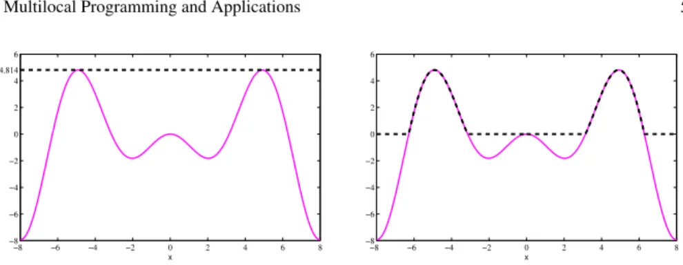
provided to show the deflected effect.
Example 1.Consider the one-dimensional problem where the objective function is
f(x) =−xsin(x), for x∈[−8,8],
which has 3 maxima in the set[−8,8].
Figure 1 shows the plot of f(x)using a solid line. Letx∗=−4.9132 be the first
computed maximizer, where f(x∗) =4.8145. The plot of the deflecting function (4)
atx∗=−4.9132 is shown with a dashed line in the left plot, where all the values
with f(x)< f(x∗)are deflected. All the maximizers are alleviated and the
func-tion becomes a line when the deflecting funcfunc-tion technique is applied on a global
maximizer. In the right plot, the deflecting technique is applied to f at the local
maximizerx∗=0, with f(x∗) =0 and as can be seen fd(x), represented by a dashed
−8 −6 −4 −2 0 2 4 6 8 −8
−6 −4 −2 0 2 4 4.814 6
x
−8 −6 −4 −2 0 2 4 6 8 −8
−6 −4 −2 0 2 4 6
x
Fig. 1 Plot offandfdatx∗=−4.9132 (left plot) and atx∗=0 (right plot).
On the other hand, the function stretching technique consists of a two-phase transformation [38, 39, 40]. The first transformation stretches the objective function downwards in a way that all the maxima with smaller values than the previously detected maximum are eliminated. Then, the second phase transforms the detected maximum into a minimum. All the other maxima (with larger values than the
de-tected maximum) are unaltered. Ifx∗is an already detected maximum of f, then the
first transformation is defined by
f1(x) =f(x)−δ1
2 kx−x
∗k[sign(f(x∗)−f(x)) +1] (5)
and the second by
f2(x) =f1(x)−δ2
[sign(f(x∗)−f(x)) +1]
2 tanh(κ(f1(x∗)−f1(x)))
(6)
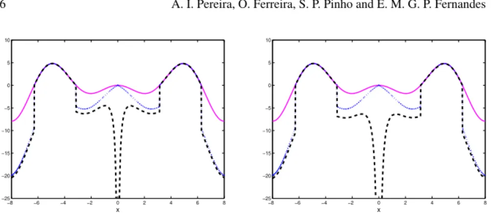
where δ1,δ2andκ are positive constants. To illustrate the effects of these
trans-formations as the parameters vary, we use Example 1. Figure 2 shows the plot of
f(x)using a solid line. Based on the computed local maximizerx∗=0 and applying
the transformation (5) withδ1=1.5, we get the function f1(x)which is plotted in
the figure with a dotted line, and applying (6), with δ2=0.5 we get the function
f2(x), displayed in both plots of the figure with a dashed line. The plot on the left
corresponds toκ=0.1 and the one on the right corresponds toκ=0.05. Function
f1(x)comes out after the first transformation (5) and the bigger theδ1the greater
the stretch is. See the plots on the right of Figs. 2 and 3. Parameterδ2defines the
range of the effect (see the plots on the left of Figs. 2 and 3) and the parameterκ
defines the magnitude of the decrease on f atx∗(see both plots of Fig. 2).
In a multilocal programming context, global as well as local (non-global) solu-tions need to be computed. Implementing the function stretching technique locally
aims at stretching downwards the objective function f only in a neighborhood of
−8 −6 −4 −2 0 2 4 6 8 −25
−20 −15 −10 −5 0 5 10
x
−8 −6 −4 −2 0 2 4 6 8
−25 −20 −15 −10 −5 0 5 10
x
Fig. 2 Plot off,f1,f2withδ1=1.5,δ2=0.5,κ=0.1 (on the left) andκ=0.05 (on the right).
−8 −6 −4 −2 0 2 4 6 8
−25 −20 −15 −10 −5 0 5 10
x
−8 −6 −4 −2 0 2 4 6 8
−25 −20 −15 −10 −5 0 5 10
x
Fig. 3 Plot off,f1,f2withδ1=1.5,δ2=1.5,κ=0.1 (on the left) andδ1=3,δ2=0.5,κ=0.05
(on the right).
global and local solutions are required since the strategy alleviates only the detected solutions. We now accept that the following assumption holds.
Assumption 1 All optimal solutions of problem (3) are isolated points.
Here we present a proposal that applies locally the function stretching technique and uses a simulated annealing algorithm. The method is able to detect sequen-tially the global and local solutions instead of rambling over the feasible region attracted by previously identified solutions. After the computation of a solution, the objective function of the current problem is transformed using the function stretch-ing technique. A sequence of global optimization problems with stretched objective functions is iteratively defined and solved by the SA algorithm [44, 45].
The main steps of the ASA algorithm are resumed in Algorithm 1 below. For details on the algorithm convergence analysis, see [23, 24]. The ASA method can be easily described using five phases: the generation of a trial point, the ‘acceptance criterion’, the redefinition of the control parameters, the reduction of the control parameters and the stopping condition.
Algorithm 1ASA algorithm
1:Given: x0,Nc0and the initial control parameter values. Setk=0 andj=0
2:Whilethe stopping condition is not verifieddo
2.1 Based onxk, randomly generate a trial pointy∈[l,u]andj=j+1
2.2 Verify the ‘acceptance criterion’
2.3 If j<Nk
c then j=j+1 and go to 2.2
elseupdateNk
candj=0
2.4 Update control parameters
2.5 Setk=k+1
The generation of a trial point is one of its crucial phases and it should provide a good exploration of the search region as well as a feasible point. The parameter Nk
cin the Algorithm 1 aims at adapting the method to the problem. The ‘acceptance
criterion’ allows the ASA algorithm to avoid getting stuck in local solutions when searching for a global one. For that matter, the process accepts points whenever an increase of the objective function is verified
xk+1=
y ifξ ≤Axk,y(ckA)
xk otherwise
wherexk is the current approximation to the global maximum,yis the trial point,
ξ is a random number drawn fromU(0,1)andAxk,y(ckA)is the acceptance function.
This function represents the probability of accepting the pointywhenxkis the
cur-rent point, and it depends on a positive control parameterckA. An usual acceptance
function is
Axk,y(ckA) =min
(
1,e−
f(xk)−f(y) ck
A
)
,
known as Metropolis criterion. This criterion accepts all points with objective
func-tion values equal or greater than f(xk). However, if f(y)< f(xk), the pointymight
be accepted with some probability. During the iterative process, the probability of descent movements decreases slowly to zero. Different acceptance criteria are
pro-posed in [24]. The control parameter ckA, also known as temperature or cooling
stopping criterion limits the number of function evaluations, or defines a lower limit for the value of the control parameter.
We now describe the details concerning the SSA algorithm. The local application of the function stretching technique aims to prevent the convergence of the ASA
al-gorithm to previously detected solutions. Letx1∗be the first detected solution.
Func-tion stretching technique is then applied only locally, in order to transform f(x)in
a neighborhood ofx∗1,Vε1(x1∗), with radiusε1>0. Thus, f(x)is reduced only inside
the regionVε1(x∗1)leaving all the other maxima unchanged. The maximum f(x∗1)
disappears but all the others remain unchanged. Each global optimization problem of the sequence is solved by ASA. The multilocal procedure terminates when, for a predefined set of consecutive iterations, no more solutions are detected [42, 44]. To illustrate this SSA procedure the following problem is considered.
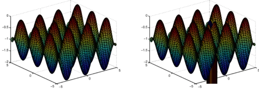
Example 2.Consider the function
f(x) =−cos2(x1)−sin2(x2) wherex∈[−5,5]2,
which has 12 global maxima in the set [−5,5]2. In Fig. 4, the objective function
of Example 2 and the function f2that comes out after applying transformations (5)
and (6) to the previously computed global maximizerx1∗, defined by(π2,0), are
dis-played. Transformations (5) and (6) stretch the neighborhood ofx∗1, with radiusε1,
downwards assigning smaller function values to those points to prevent convergence to that previously computed solution [44]. As can be observed, the other maxima are left unchanged (see Fig. 4).
−5 0
5
−5 0 5 −2 −1.5 −1 −0.5 0
−5 0
5
−5 0 5 −2 −1.5 −1 −0.5 0
Fig. 4 Plot off(x)(left) andf2(x)(right) in Example 2.
Thus, the SSA method, at each iteration, solves a global programming problem using the ASA algorithm, where the objective function of the problem resulted from a local application of the function stretching technique that aims to eliminate the pre-viously detected maximizer leaving the other maximizers unchanged. This process is repeated until no other solution is encountered. The mathematical formulation of
max
l≤x≤uf j+1(x)
≡
f2j(x)ifx∈Vεj(x∗j),
fj(x)otherwise (7)
wherex∗jis the solution detected in the j-order problem, and the following notation
is used: f2j is the stretched function obtained from fjafter transformations (5) and
(6), for any j, where f1=f, and f21= f2.
Algorithm 2 below presents, in summary, the strategy SSA for MPP (3). As pre-viously stated the algorithm terminates when no more solutions are detected during
a predefined number of consecutive iterations,Kiter, or a maximum number of
func-tion evaluafunc-tions is reached,n fmax. The conditions for the inner cycle (in Step 2.2)
aim at defining an adequate radius (εj) for the neighborhood of each solution
com-puted in Step 2.1, in order to adjust for eachx∗j the convenient neighborhood. In the
final stage of the algorithm, a local search procedure is applied to each computed solution to improve accuracy.
Algorithm 2SSA algorithm
1:Given:δ0,ε0,εmax. Setfmax=f1(l), j=1 andp=0
2:Whilethe stopping conditions are not metdo
2.1 Computex∗j=arg maxl≤x≤ufj(x)using Algorithm 1 withfj(x)defined in (7)
2.2 Set∆=ε0
2.3 While
fj(x∗
j)−fmax
≤δ0 or ∆>εmaxdo
Setp=p+1 and∆=pε0
Randomly generateexi∈V∆(x∗j),i=1, . . . ,2n
Findfmax=maxi=1,...,2n{fj(xei)}
2.4 Update the optimal setX∗and setεj=∆
2.5 Setj=j+1 andp=0
3: Apply a local search procedure to the optimal setX∗
Example 3.Consider the classical optimization problem known as Branin prob-lem [20].
max f(x)≡ −
x2−
5.1 4π2x
2 1+
5
πx1−6
2
−10
1− 1
8π
cos(x1)−10,
where the feasible region is defined asF=x∈R2:−5≤x
1≤10∧0≤x2≤15 .
This problem has three global maximizers(−π,12.2750),(π,2.2750)and(9.4248,
2.475)with a maximum value of−0.39789.
The SSA algorithm solves this problem in 0.45 seconds, needs 2442 function
evaluations and detects the following maximizers(−3.1416E+00,1.2275E+01),
(9.4248E+00,2.4750E+00)and(3.1416E+00,2.2750E+00), with global value
was solved thirty times. In this case all the solutions were identified in all runs. The results were obtained using a Intel Core 2 Duo, T8300, 2.4 GHz with 4 GB of RAM.
The parameters of the algorithm are set as follows:δ0=5.0,ε0=0.1,εmax=1.0,
Kiter=5 andn fmax=100 000.
2.2 Deterministic methods
Deterministic methods for global optimization are able to solve a problem with a re-quired accuracy in a finite number of steps. Unlike stochastic methods, the outcome of the algorithm does not depend on pseudo random variables. In general, they pro-vide a theoretical guarantee of convergence to a global optimum. When compared to stochastic methods, they may rely on structural information about the problem and, in some cases, they require some assumptions on the objective function such as, for
example, the Lipschitz continuity of f over the feasible region [14, 20, 21, 31].
There are deterministic methods that combine the branch-and-bound method with successive refinement of convex relaxations of the initial problem [15], others use a non-differentiable technique based on the method of optimal set partitioning [27], and in [28] partitioning ideas are combined with some derivative information. An important subclass of methods for locating the solutions (maximizers and mini-mizers) of a continuous function inside bound constraints, like problem (3), consist of two phases: first, a partition of the feasible set is made and a set of finite points are generated and evaluated in order to detect good approximations to solution points; then, a local search method is applied in order to improve the accuracy of the ap-proximations found in the first phase (e.g. [10, 11, 48, 51]).
DIRECT is a deterministic method that has been designed to find the global so-lution of bound constrained and non-smooth problems where no derivative informa-tion is needed [14, 25, 26]. DIRECT is an acronym for DIviding RECTangles and is designed to completely explore the search space, even after one or more local solu-tion have been identified. The algorithm begins by scaling the domain into the unit hypercube and the objective function is evaluated at the center of the domain, where an upper bound is constructed. DIRECT computes the objective function at points that are the centers of hyperrectangles. At each iteration, new hyperrectangles are formed by dividing those that are more promising, in the sense that they potentially contain a required global solution, and the objective function is evaluated at the cen-ters of those hyperrectangles. Based on those objective function values, the method is able to detect new promising hyperrectangles.
Another interesting subclass of deterministic methods for global optimization is based on the idea of branch and bound. Methods based on interval analysis [2, 19, 61] fall in this subclass. Interval analysis arises from the natural extension of real arithmetical operations to interval operations. Its use for global optimization was presented in 1992 [19]. Using interval operations, the interval algorithm splits,
successively, the initial feasible region[l,u]into small subintervals. The subintervals
subdi-vided and analyzed. This process terminates when the width of the subintervals are below a predefined accuracy or no interval remains to be subdivided. Interval meth-ods have high computational costs since the complexity rises exponentially with the dimension of the problem [19, 20].
The most known and used deterministic method is the branch-and-bound (BB) method. It has been mainly used in discrete optimization. The main idea in a BB method is the recursive decomposition of the original problem into smaller disjoint subproblems until the required solution is detected. In this context, smaller means either a strict smaller problem dimension or a strict smaller feasible region. The partition of the feasible region is the most used branching rule in continuous pro-gramming. This decomposition should guarantee that the global solution is at least in one of the generated subproblems. The method compares the lower and upper bounds for fathoming each subregion. The subregion that contains the optimal so-lution is found by eliminating subregions that are proved not to contain the optimal solution.
BB-type methods are characterized by four natural rules: branching, selection, bounding and elimination. Branching is concerned with further refinement of the partition. The selection rule is also very important, greatly affects the performance of the algorithm and aims at deciding which subregion should be explored next.
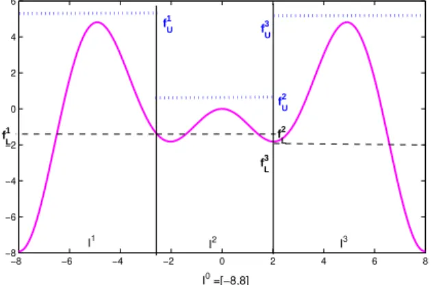
The method starts with a setI0that contains the feasible region assumed to be a
compact set. An algorithm should be provided to compute an upper bound value,fU,
such thatfU≥f(x)for allx∈[l,u]that will be improved as subproblems are solved.
At each iteration, the method has a listL of subsetsIkofI0. An upper bound fk
U
of the maximum objective function value onIkis computed for every subset inL.
A global lower bound fLof the maximum function value over the feasible region is
defined by the f value of the best feasible solution found.
−8 −6 −4 −2 0 2 4 6 8
−8 −6 −4 −2 0 2 4 6
f3 U f1U
f2U
f2L
I1 I3
I0 =[−8,8] I2
f1 L
f3L
Fig. 5 Branching applied to the continuous Example 1.
Figure 5 illustrates a branching rule applied to the function in Example 1. The
line. The lower bounds, fLk, are the higher function values at the boundaries of the
subintervals and are represented by dashed lines. The upper bounds, fUk, represented
in the figure by dotted lines, are computed using a simple procedure. In this case, all the subintervals should be explored and subdivided again by the branching rule, since no upper bound is lower than any lower bound.
A subregionIkcan be removed from the listL if:
i) it cannot contain any feasible solution;
ii) it cannot contain the optimal solution since fUk< fL;
iii)there is no use in splittingIksince the size of the set is smaller than a predefined
toleranceδ.
A crucial parameter of the BB method is the positive δ-precision. This
tole-rance is used in the stopping criteria in a way that a solution within aδ-precision is
obtained. The algorithm also stops when the listL is empty. When solving discrete
problems, the parameterδcan be set to zero and the BB algorithm is finite. However,
in continuous optimization, the bounding operation is required to be consistent, i.e.,
any infinitely decreasing sequence of successive refined partitionsIkonI0satisfies
lim
k→∞(f
k
L−fUk) =0
where fLkand fUk are the lower and upper bounds, respectively, of the problem with
feasible regionIk. This consistency condition implies that the requiredδ-precision
solution is achieved after a finite number of steps and the BB algorithm is therefore finite.
In the multilocal programming context, to compute the solutions of (3), the BB method is combined with strategies that keep the solutions that are successively identified during the process. The method also avoids visiting those subproblems which are known not to contain a solution [20, 21]. The main step of the proposed multilocal BB method is to solve a sequence of subproblems described as
maxf(x)for x∈Ii,j andi=1, . . . ,nj (8)
whereIi,j= [li1,j,ui1,j]× ··· ×[lni,j,uin,j], and the subsetsIi,j, fori=1, . . . ,nj, belong
to a list, herein denoted byLj, that can have a local solution that satisfies condition
(2).
The method starts with the listL0, with the setI1,0= [l,u], as the first element
and stops at iteration j, when the listLj+1is empty. The generic scheme of the
multilocal BB algorithm can be formally described as shown in Algorithm 3. Fur-thermore, the algorithm will always converge due to the final check on the width of
the subintervalIi,j(see the stopping conditions in Step 3 of the algorithm). A fixed
value,δ>0, is provided in order to guarantee aδ-precision solution.
To illustrate the practical behavior of Algorithm 3, the problem presented in
Ex-ample 3 is used. The multilocal BB algorithm solves this problem in 37.1 seconds,
needs 9331 function evaluations and finds the following maximizers (3.1416E+
Algorithm 3Multilocal BB algorithm
1:Given:δ0>0,δ>0
2: Considerf0the solution of problem (8), forI1,0= [l,u], setj=0 andn0=1
3:While Lj+16=/0 and max
iui,j−li,j
≥δ do
3.1 Split each setIi,jinto intervals, fori=1, . . . ,nj; setLj+1=
I1,j+1, . . . ,Inj+1,j+1 3.2 Solve problem (8), for all subsets inLj+1.
3.3 Setf1, . . . ,fnj+1to the obtained maxima values
3.4 Setf0=maxi
fi fori=0, . . . ,nj+1. Select the subsetsIi,j+1that satisfy the condition:
f0−fi<δ0 3.5 Reorganize the listLj+1; updaten
j+1
3.6 Setj=j+1
00)with global value−3.9789E−01. As expected, the multilocal BB algorithm is
computationally more demanding than the SSA algorithm.
2.3 Numerical experiments
This subsection reports the results of applying Algorithm 2 to solve bound con-strained MPP. The Algorithm 3 was not used because it is high time consuming. First, an experiment with a varied dimensional problem is analyzed for five
differ-ent values ofn. Then, a large dimensional problem is solved by the SSA algorithm.
The problems were solved using a Intel Core 2 Duo, T8300, 2.4 GHz with 4 GB
of RAM. The parameters in the algorithm are set as follows:δ0=20.0,ε0=0.1,
εmax=1.0,Kiter=5 andn fmax=100 000.
2.3.1 Experiment with a varied dimensional problem
Example 4.Consider the classical optimization problem known asn-dimensional
Test (n-dT) [12]:
maxf(x)≡ −12
n
∑
i=1
(x4i−16x2i+5xi) +ϖ n
∑
i=1
(xi−2.90353)2
s.t.−5≤xi≤5,i=1, . . . ,n
forϖ=0 (classical problem) andϖ=0.3 (modified). This problem has 2nlocal
maxima in the set[−5,5]nand the global is located at(−2.9035, . . . ,−2.9035). The
2-dT function for the classical problem withn=2 is plotted in Fig. 6. The global
are located at(−2.9036,2.7468)(with f =64.196),(2.7468,−2.9035)(with f =
64.196) and(2.7468,2.7468)(withf =50.059).
−5
0
5
−5 0 5 −200 −150 −100 −50 0 50 100
x1
−0.5 (x
1 4 − 16 x
1 2 + 5 x
1 +x2 4 − 16 x
2 2 + 5 x
2)
x
2
−5 −4 −3 −2 −1 0 1 2 3 4 5 −5
−4 −3 −2 −1 0 1 2 3 4 5
Fig. 6 Plot of the classical 2-dT problem.
Results regarding the classical problem in Example 4 forn=2,4,6,8,10 are shown
in Table 1. The table depicts a summary of the results obtained by the SSA algo-rithm. The average value of the solutions found for the global maximum, in all the
runs, favg∗ , the average number of function evaluations (obtained in all 30 runs, when
computing the global),n favgeval, the average (over all runs) of the CPU time required
to converge to all the solutions identified by the algorithm (in seconds), CPU(s), the
best solution found for the global maximum during the 30 runs, f∗, and the average
number of solutions identified by the algorithm,nsol, are displayed. Table 2 reports
the same results for the modified problem (ϖ=0.3) in Example 4. The SSA
al-gorithm was able to identify several maximizers during the process, in both tested problems (classical and modified), although not all maximizers are detected in all runs. We may conclude that the efficiency of the algorithm is not greatly affected by the dimension of the problem.
Table 1 Results of the SSA algorithm for Example 4, consideringϖ=0.
Problem favg∗ n feval
avg CPU(s) f∗ nsol
2-dT 7.8332E+01 1067 0.17 7.8332E+01 2
4-dT 1.5667E+02 3159 0.29 1.5667E+02 2
6-dT 2.3500E+02 10900 0.75 2.3500E+02 2
8-dT 3.1333E+02 36326 2.28 3.1333E+02 1
Table 2 Results of the SSA algorithm for Example 4, consideringϖ=0.3.
Problem favg∗ n feval
avg CPU(s) f∗ nsol
2-dT 9.8911E+01 1386 0.34 9.8911E+01 2
4-dT 1.9782E+02 2796 0.25 1.9782E+02 2
6-dT 2.9673E+02 10110 0.69 2.9673E+02 1
8-dT 3.9426E+02 30641 1.95 3.9426E+02 1
10-dT 4.9456E+02 56604 3.58 4.9456E+02 1
2.3.2 Experiment with a large dimensional problem
Here we analyze the performance of the SSA algorithm when solving a large di-mensional MPP.
Example 5.Consider the following optimization problem with a multimodal objec-tive function [30]:
maxf(x)≡ −
n
∑
i=1
sin(xi) +sin
2xi
3
s.t. 3≤xi≤13,i=1, . . . ,n
which has an analytical global optimum of 1.216n. Figure 7 contains the plot of
f(x)whenn=2. The global maximizer is located at(5.3622,5.3622). The other
maximizers in [3,13]2 are: (10.454,5.3622)(with f =1.4393),(5.3622,10.454)
(with f =1.4393) and(10.454,10.454)(with f =0.4467). The other optimum is
a minimum with f=−0.4467 at(8.3961,8.3961). Table 3 contains the results
ob-tained by the SSA algorithm for two different values ofn: 50 and 100. Clearly, the
SSA algorithm is able to solve large-dimensional problems, detecting some solu-tions, in a reasonable time. The number of function evaluations and the CPU time
are smaller in the case ofn=100. We remark that these results were obtained with
n fmax=1 000 000.
Table 3 Results of the SSA algorithm for Example 5.
n favg∗ n feval
avg CPU(s) f∗ nsol
50 6.0799E+01 944761 287 6.0799E+01 4
4 6
8 10
12
4 6 8 10 12 −3 −2 −1 0 1 2 3
x
1
−(sin(x
1)+sin(x2)+sin(2 x1/3)+sin(2 x2/3))
x2 3 4 5 6 7 8 9 10 11 12 13
3 4 5 6 7 8 9 10 11 12 13
Fig. 7 Plot off(x)of Example 5 forn=2.
3 Constrained Multilocal Programming
In general, constrained optimization problems are more difficult to solve than un-constrained or bound un-constrained problems, specially when the feasible region is not convex and is very small when compared with the whole search space. There is a
metricρgiven by the ratio between the feasible region and the search space that can
be used to measure the difficulty of solving a problem. With a stochastic method,
ρ can be estimated by the ratio between the number of feasible solutions and the
total number of solutions randomly generated [29]. Feasible regions made of dis-jointed regions are also difficult to handle, in particular by gradient-based methods. Stochastic methods are in general well succeeded when solving this type of difficult problems. Different constrained search spaces have motivated the development of a variety of constraint-handling techniques. The three main classes of methods to handle constraints are:
• methods that use penalty functions;
• methods based on biasing feasible over infeasible solutions;
• methods that rely on multi-objective optimization concepts.
We refer the reader to [34, 54] and to the references therein included. There are also other techniques that aim at repairing infeasible solutions. In [60], a method that uses derivative information from the constraint set to repair infeasible points is proposed in a hybrid particle swarm optimization context.
Penalty function-based methods are the most well-known class of methods to handle constraints in nonlinear optimization problems. These techniques transform the constrained problem into a sequence of unconstrained subproblems by
penal-izing the objective function f whenever constraints are violated. Then, the goal is
func-tion of the problem, a penalty term and a (at least one) positive penalty parameter. This is an iterative process where the solutions of the unconstrained subproblems are approximations to the solution of the constrained problem.
To solve the constrained MPP in the form presented in (1), some theory and practice of penalty methods is addressed in the remaining part of this section.
3.1 The penalty function method
A variety of sophisticated penalties exist in the class of penalty function meth-ods [20, 36, 57]. They were developed to efficiently address the issue related with constraint-handling in problems with different structures and types of constraints. Additive penalties define a penalty function of the form
φ(x;µ) =f(x)−P(g(x),µ)
where f(x)is the objective function in problem (1) andP, known as the penalty
term, depends on the constraint functionsg(x)and a positive penalty parameterµ.
The penalty term should be zero when the point is feasible and thenφ(x;µ) =f(x),
and is positive when the point is infeasible. The penalty term aims at penalizing the constraint violation, directing the search towards the feasible region and, at the same
time, looking upwards for a point with the largest f. On the other hand,
multiplica-tive penalties have the form
φ(x;µ) =f(x)Pmult(g(x),µ)
wherePmult(g(x),µ)is a function that should take the value one when the point is
feasible and smaller than one for infeasible points. There is no special rule to design a penalty function. Experiments show that penalties that depend on the distance from feasibility are better than those that rely on the number of violated constraints alone.
whole population of points. Adaptive penalties are proposed in [5] in conjunction with a genetic algorithm. A penalty adapting algorithm used with an ant colony op-timization aiming at eliminating the need for trial-and-error penalty parameter de-termination is proposed in [1]. We refer to [9] for details concerning these penalties, advantages and drawbacks during implementation.
Another common classification of penalty functions in classical optimization is based on interior and exterior penalty functions [6, 7]. Exterior penalties are used more often than interior penalties since an exterior penalty function does not require an initial feasible point to start the iterative process. Furthermore, algorithms based on interior penalty functions are more complex since all generated points should be maintained inside the feasible region throughout the whole iterative process. A well-known interior penalty is the logarithmic barrier function and works only with inequality constraints.
Here, we are specially interested in exterior penalty functions of the additive type. Three different penalty functions are described and tested with a benchmark set of problems. Although setting the initial value for the penalty parameter as well as its updating scheme are usually critical in algorithm’s performance, they are not yet well-defined issues. Nevertheless, these issues are addressed since convergence to the solution is to be promoted and accelerated. Thus, details concerning the most appropriate strategies for updating the penalty and other related parameters are pre-sented.
Our implementation of the penalty framework intends to penalize only the in-equality constraints. Each subproblem of the sequence that is solved for a fixed
value of the penaltyµis the bound constrained multilocal optimization problem
maxφ(x;µ)
s.t.li≤xi≤ui,i=1, ...,n (9)
To illustrate the effect on the penalty function φ as the penalty parameterµ
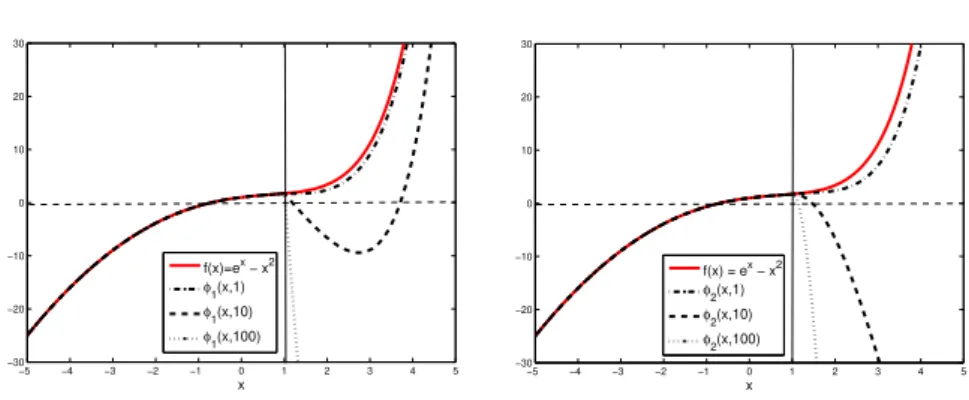
in-creases, a one-dimensional example is used.
Example 6.Consider the problem
maxf(x)≡ex−x2 s.t. x≤1 andx∈[−5,5].
Figure 8 shows, on the left plot, the penalty functionφ1that depends on the penalty
termP(x,µ) =µmax{0,x−1}and, on the right plot, theφ2that depends on the
penalty termP(x,µ) =µ(max{0,x−1})2, for the three values ofµ=1,10,100.
As can be seen, in the feasible region[−5,1], the penalty function coincides with
f(x), the functionφ2is smoother atx=1 (the solution of the problem) thanφ1, and
the larger theµthe more difficult the problem is.
L1/2 penalty function. A variant of a dynamic nonstationary penalty function is herein used to solve constrained MPP [30, 41]. In these papers, particle swarm op-timization algorithms are implemented in conjunction with the penalty technique.
−5 −4 −3 −2 −1 0 1 2 3 4 5 −30 −20 −10 0 10 20 30 x f(x)=ex − x2
φ1(x,1)
φ1(x,10)
φ1(x,100)
−5 −4 −3 −2 −1 0 1 2 3 4 5 −30 −20 −10 0 10 20 30 x f(x) = ex − x2
φ2(x,1)
φ2(x,10)
φ2(x,100)
Fig. 8 Plot off(x)andφ1(on the left) andφ2(on the right) relative to Example 6.
is defined as
P1/2(x,µ) =µ
m
∑
j=1
max0,gj(x) γ
(gj(x))
(10)
where the power of the constraint violation, γ(.), may be a violation dependent
constant. The simplest approach setsγ(z) =1 ifz≤0.1, andγ(z) =2, otherwise.
This is a nonsmooth function and derivative-free methods should be applied when solving problem (9). Unlike the suggestions in [30] and [41], the penalty parameter in (10) will not be changing dynamically with the iteration number. To define an
appropriate updating scheme for µ, one has to consider a safeguarded scheme to
prevent the subproblems (9) from becoming ill-conditioned as the penalty parameter
increases [7]. An upper boundµmaxis then defined and the update is as follows:
µk+1=
minnτµk,µmax
o
,forτ>1 andµmax>>1, (11)
given an initial value µ0>0, wherek represents the iteration counter. Thus, the
sequence of solutions{x∗(µk)}, from (9), will converge to the solutionx∗of (1) and
φ(x∗(µk);µk)→ f(x∗)ask→∞.
L2-exponential penalty function. We now extend the use of a continuous l2
-exponential penalty function to the constrained multilocal optimization problem. This penalty function was previously incorporated into a reduction-type method for solving semi-infinite programming problems [43]. The penalty term depends on the
positive penalty parameterµand two other fixed positive parametersν1,ν2:
Pexp
2 (x,ν1,ν2,µ) =
ν1
µ
eµθ(x)−1
+ν2
2
eµθ(x)−1
2
, (12)
whereθ(x) =maxj=1,...,m[gj(x)]+and the[gj(x)]+represents max{0,gj(x)}. Clearly,
θ(x)is the infinity norm of the constraint violation. The tuning of the penalty
Hyperbolic penalty function.Another proposal uses the 2-parameter hyperbolic penalty function [56]. This is a continuously differentiable function that depends on
two positive penalty parameters, in general different for each constraint, µ1,j and
µ2,j, j=1, . . . ,m,
Phyp(x,µ1,µ2) =
m
∑
j=1
µ1,jgj(x) +
q
µ2
1,j[gj(x)]2+µ22,j. (13)
This penalty works as follows. In the initial phase of the process, µ1 increases,
causing a significant increase of the penalty at infeasible points, while a reduction in penalty is observed for points inside the feasible region. This way the search is directed to the feasible region since the goal is to minimize the penalty. From the
moment that a feasible point is obtained, the penalty parameterµ2decreases. Thus,
the parametersµ1,jandµ2,jare updated, for each j=1, . . . ,m, as follows:
(
µk+1
1,j =τ1µ1k,jandµ k+1
2,j =µ2k,j, if max{0,gj(xk)}>0
µk+1 2,j =τ2µ
k
2,jandµ1k,+j1=µ k
1,j, otherwise
for each j=1, . . . ,m, whereτ1>1 andτ2<1.
Multilocal penalty algorithm.The multilocal penalty (MP) algorithm can be im-plemented using the stretched simulated annealing algorithm when solving subprob-lem (9), or the multilocal BB, both previously described in Subsections 2.1 and 2.2, respectively. Details of the main steps of the algorithm are shown in Algorithm 4. The algorithm is described for the simpler penalty function, see (10). Adjustments have to be made when the penalty functions (12) and (13) are used.
Algorithm 4MP algorithm
1: Given:µ0,µmax,τ,δ0,ε0,εmax. Setk=0
2: Whilethe stopping conditions are not metdo
3: SetLk=0 andj=0
4: Whileinner stopping conditions are not metdo
4.1 Setp=0 andj=j+1
4.2 Computex∗j(µk) =arg max
l≤x≤uφj(x;µk)using Algorithm 2 or Algorithm 3
4.3 While
φj
x∗j(µk),µk
−φemax
≤δ0or∆>εmaxdo
Setp=p+1 and∆=pε0
Randomly generateexi∈V∆(x∗j),i=1, . . . ,2n
Findφemax=maxi=1,...,2n{φj(exi,µk)}
4.4 SetLk=Lk+1 andε
j=∆
5: µk+1=min{τµk,µ
3.2 Numerical experiments
Here, we aim to compare the effectiveness of the SSA algorithm when coupled with a penalty function method to compute multiple solutions. The above listed penalty
functions, l1/2penalty, l2-exponential penalty and the hyperbolic penalty are tested.
Stopping conditions.The stopping conditions for the multilocal penalty algorithm
are:
X∗(µk)−X∗(µk−1)≤εx ork>kmax
and the inner iterative process (in Step 2 of Algorithm 4) terminates ifLkdoes not
change for a specified number of iterations,Kiter, or a maximum number of function
evaluations is reached,n fmax.
Setting parameters. In this study, the selected values for the parameters resulted
from an exhaustive set of experiments. Here is the list:εx=10−3,kmax=1000 and
the parameters for the l1/2penalty function areµ0=10,µmax=103andτ=10. The
parameters used in the l2-exponential penalty function areν1=100 andν2=100.
The parameters used in the Hyperbolic penalty function are µ10,j=µ0
2,j=10 for
j=1, . . . ,m,τ1=
√
10 and τ2=0.1. The parameters of the SSA algorithm are
set as follows:δ0=5.0,ε0=0.1,εmax=1.0,Kiter=5 andn fmax=100 000. The
problems were solved in a Intel Core 2 Duo, T8300, 2.4 GHz with 4 GB of RAM.
Experiments. For the first part of our comparative study, we use a well-known problem described in Example 7.
Example 7.Consider the camelback objective function
f(x) =−
4−2.1x21+x
4 1
3
x21−x1x2+4(1−x22)x22
which has four local maxima and two minima in the set−2≤xi≤2,i=1,2. The
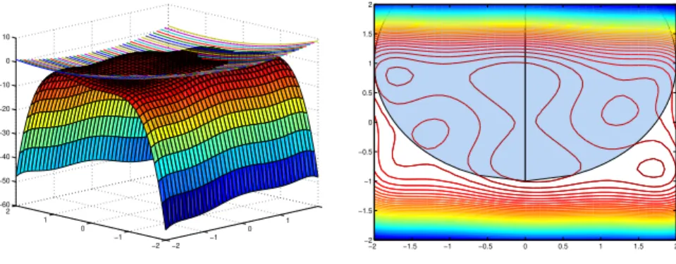
two global maxima are located at (0.089842, -0.712656) and (-0.089842, 0.712656). Here, we define the constrained problem:
max f(x)
s.t.g(x)≡x21+ (x2−1)2−4≤0,
−2≤xi≤2,i=1,2
(14)
and illustrate the behavior of the MPA when using SSA algorithm to solve the bound
constrained subproblems. Figure 9 shows the 3D plot and contour lines of f(x)as
well as ofg(x)≤0. This nonconvex problem has three maxima in the interior of the
feasible region.
The problem in (14) was solved using the MP algorithm combined with the
hy-perbolic penalty function. The method identified two global solutions(−8.9842E−
−2 −1
0 1
2
−2 −1 0 1 2 −60 −50 −40 −30 −20 −10 0 10
−2 −1.5 −1 −0.5 0 0.5 1 1.5 2 −2
−1.5 −1 −0.5 0 0.5 1 1.5 2
Fig. 9 Plot off(x)andg(x)≤0 in Example 7.
00. The local maximizer(−1.7036E+00,7.9608E−01)with value 2.1546E−01
was also detected. To solve this problem, the MP algorithm needed 2.14 seconds of
CPU time and 10535 functions evaluations, both average numbers in 30 runs. To further analyze the performance of the multilocal penalty algorithm when coupled with SSA, a set of six benchmark problems, described in full detail in [29],
is used. In this study, small dimensional problems (n≤10 and m≤13) with a
nonlinear objective function, simple bounds and inequality constraints were tested. They are known in the literature as g04, g06, g08, g09, g12 and g18. Details of the selected problems are displayed in Table 4, where ‘Problem’ refers to the problem
number, ‘type of f(x)’ describes the type of objective function, ‘fopt-global’ is the
known global solution (all are minimization problems),nis the number of variables
andmis the number of inequality constraints.
Table 4 Details of the constrained problems selected from [29].
Problem type off(x) fopt-global n m
g04 quadratic −3.0665E+04 5 6
g06 cubic −6.9618E+03 2 2
g08 general −9.5825E−02 2 2
g09 general 6.8063E+02 7 4
g12 quadratic 1.0000E+00 3 1
g18 quadratic −8.6603E−01 9 13
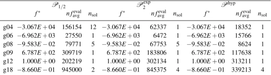
Table 5 contains the results obtained with the penaltiesP1/2,Pexp
2 andP hyp,
when combined with the SSA algorithm. The f∗is the best solution found for the
global minimum during all the 30 runs,n favgevalindicates the average number of
func-tion evaluafunc-tions required to obtain the global minimum (over the 30 runs) andnsol
Table 5 Results for the MP algorithm, combined with SSA.
P1/2 Pexp
2 Phyp
f∗ n feval
avg nsol f∗ n favgeval nsol f∗ n favgeval nsol
g04 −3.067E+04 156154 12 −3.067E+04 62337 1 −3.067E+04 18352 1
g06 −6.962E+03 27550 1 −6.962E+03 6472 1 −6.962E+03 15766 1
g08 −9.583E−02 79771 5 −9.583E−02 67753 5 −9.583E−02 8624 1
g09 6.787E+02 309719 1 6.787E+02 183806 1 6.787E+02 117638 1
g12 1.000E+00 202219 1 1.000E+00 302134 1 1.000E+00 313211 1
g18 −8.660E−01 945000 2 −8.660E−01 845375 4 −8.660E−01 339213 4
4 Engineering Applications
In the last part of the chapter, an application of multilocal programming in the engi-neering field is presented. Phase stability studies are multilocal programming prob-lems frequently found in the chemical engineering area with special interest in pro-cess design and optimization. These studies, still a current subject for scientists and engineers, are specially difficult, since the feasible region is very small and not con-vex. In this section the mathematical formulation of the problem is initially given as well as a very brief summary of the strategies and optimization techniques used so far. Following, some numerical results are presented and discussed, and the main findings outlined.
4.1 Phase stability
Separation processes are fundamental and ubiquitous operations in the chemical based industries. However, to design and optimize such separation operations, ther-modynamic equilibrium conditions must be known. A severe problem causing enor-mous difficulties in this regard is that the number and identity of phases present at equilibrium are generally not known [46], which makes phase stability analysis obligatory. At a fixed temperature, pressure and global composition the problem is, therefore, to evaluate if the system is globally stable regarding the separation in two or more liquid phases.
The phase stability criteria based on the Gibbs free energy of mixing, or derived properties, are multiple, but the minimization of the tangent plane distant function (T PDF), firstly proposed by Baker et al. [4], and first implemented by Michelsen [35], is usually applied, and accepted to be a reliable and potent methodology for
stability studies. Considering the Gibbs free energy of mixing (∆G) of a
multi-component mixture, at a given temperature (T) and pressure (P), to be described
as∆g(x) =∆RTG =f(T,P,x), wherexis the vector ofnmole fraction compositions
characterizing that mixture andRis the ideal gas constant. For an initial feed
(∆gt p) at that point is
∆gt p(x) =∆g(z) + n
∑
i=1
∂∆
g
∂xi
x=z
(xi−zi).
In this way, the tangent plane distance function (T PDF) is calculated by
T PDF(x) =∆g(x)−∆gt p(x).
Among the several thermodynamic models possible to apply, NRTL model [47] is one of the most successful in the representation of equilibrium properties of mul-ticomponent liquid mixtures, and is frequently found in commercial software for process simulation and design. Therefore, NRTL model is here applied for which
∆g=
n
∑
i=1
xiln(xi) + n
∑
i=1
xi n
∑
j=1
τjiGjixj
n
∑
l=1
Glixl
whereτjiandGjiare interaction parameters between components jandi, calculated
byGji=exp(−αjiτji), beingαthe non-randomness parameter. They are all readily
available in the open literature.
To evaluate if a mixture of a given global composition shows phase instability the following nonlinear multilocal optimization problem must be solved
minT PDF(x)
s.t.
n
∑
i=1
(xi)−1=0
0≤xi≤1 and i=1, . . . ,n.
The necessary and sufficient condition for stability is that at the global minimum the T PDF(x)function is nonnegative. Phase instability will be observed otherwise. In that event the following step is to find the number of phases in equilibrium as well as the composition of each phase.
Due to the mathematical complexity of the thermodynamic models, the
mini-mization of theT PDFand location of all the stationary points are demanding tasks,
requiring robust numerical methods, since these functions are multivariable, non-convex, and highly nonlinear [8]. Strictly speaking, to check phase stability only the global minimum is needed. However, the identification of all stationary points is
very important because the local minima inT PDF are good initial guesses for the
equilibrium calculations [13, 49].
state that many techniques are initialization dependent, and may fail by converg-ing to trivial solutions or be trapped in local minima [8, 13, 16, 33, 49], features which are under attention in the numerical examples given in the following pages. Hence, the performance analysis of new numerical techniques is still of enormous importance concerning phase stability and equilibria studies.
Particularly, several variants of the simulated annealing method have been widely applied, and importantly studies have been performed concerning the so-called ‘cooling schedule’, by fixing the control parameters to the best values [13, 46, 58, 66]. Naturally, a compromise must be made between efficiency and reliability, ana-lyzing the probability of obtaining the global minimum within a reasonable compu-tational effort. On the other hand, a branch and bound algorithm has been used with several thermodynamic models [59, 65]. These authors claim that it can effectively solve the global stability problem, but only a few studies have been carried out.
4.2 Numerical experiments
Due to space limitations, only two relevant examples are now presented using SSA algorithm.
Example 8.Consider the binary system water (1) + butyl glycol (2) at 5oC. It might seem a simple example, but this is a canonical example, where multiple stationary points and local solutions can be found. Additionally, for some compositions, in [37] it was concluded that the stationary points found in [17], using the interval Newton method, are not true roots as shown by the simulated annealing method.
The NRTL parameters used in the calculations are given in Table 6, while Table 7
compiles the results obtained at four different global compositionsz.
Table 6 NRTL parameters in Example 8 [17].
Components i j τi j τji αi j=αji
water/butyl glycol 1 2 1.2005955 1.4859846 0.121345
Confirming the results from [37], at the first two compositions only one stationary point was found, giving the indication that only one liquid phase will be formed. On
the contrary, the other two compositions present a negative value of theT PDF at
the global minimum, suggesting phase instability. At the global composition (0.25, 0.75) it must be noted the closeness of two stationary points, which can introduce difficulties when applying the stretched technique as well as the small magnitude of the function at the stationary point. The performance of the SSA can be assessed by
Table 7 Numerical results for the binary system water + butyl glycol.
z CPU(s) f∗ x∗
(5.00E-02, 9.50E-01) 0.22 0.0000E+00 (5.00E-02, 9.50E-01)
(1.00E-01, 9.00E-01) 0.27 0.0000E+00 (1.00E-01, 9.00E-01)
(2.50E-01, 7.50E-01) 0.30 -9.2025E-02 (8.79E-01, 1.21E-01)
0.0000E+00 (2.50E-01, 7.50E-01)
8.4999E-05 (2.96E-01, 7.04E-01)
(5.00E-01, 5.00E-01) 0.20 -3.4091E-02 (1.43E-01, 8.57E-01)
-2.7355E-02 (8.36E-01, 1.64E-01)
0.0000E+00 (5.00E-01, 5.00E-01)
point (x∗). It also must be stressed that the average time is much uniform when
comparing with the results in [37] and [17].
Example 9.Consider now the ternary system n-propanol (1) + n-butanol (2) +
wa-ter (3) at 25oC. The NRTL parameters needed are compiled in Table 8.
Table 8 NRTL parameters in Example 9 [66].
Components i j τi j τji αi j=αji
propanol/butanol 1 2 -0.61259 0.71640 0.30
propanol/water 1 3 -0.07149 2.74250 0.30
butanol/water 2 3 0.90047 3.51307 0.48
This is also a reference system in the study of phase stability, presenting, like in the previous example, multiple stationary points. Table 9 presents a complete list of
the results found for two global compositions. In both cases theT PDF function is
negative indicating phase splitting. It must again be stressed the closeness of some stationary points and the very small magnitude of the function. The average time although longer than in the previous example is still very uniform.
Table 9 Numerical results for the ternary system n-propanol + n-butanol + water.
z CPU(s) f∗ x∗
(1.20E-01, 8.00E-02, 8.00E-01) 2.42 -7.4818E-04 (5.97E-02, 2.82E-02, 9.12E-01)
-3.0693E-06 (1.30E-01, 8.91E-02, 7.81E-01)
0.0000E+00 (1.20E-01, 8.00E-02, 8.00E-01)
(1.30E-01, 7.00E-02, 8.00E-01) 2.34 -3.2762E-04 (7.38E-02, 3.03E-02, 8.96E-01)
-8.6268E-07 (1.38E-01, 7.56E-02, 7.87E-01)