M
ASTER IN
M
ONETARY AND
F
INANCIAL
E
CONOMICS
D
ISSERTATION
S
OVEREIGN
C
REDIT
R
ATING
M
ISMATCHES
A
NDRÉ
M
ASSENA DE
A
LBUQUERQUE
M
ASTER IN
M
ONETARY AND
F
INANCIAL
E
CONOMICS
D
ISSERTATION
S
OVEREIGN
C
REDIT
R
ATING
M
ISMATCHES
A
NDRÉ
M
ASSENA DE
A
LBUQUERQUE
S
UPERVISOR:
P
ROF.
D
OUTORA
NTÓNIOM
ANUELP
EDROA
FONSOM.Sc. in Monetary and Financial Economics
Supervisor: Professor Doutor António Manuel Pedro Afonso
Abstract
In this work we study the factors, among the determinants of sovereign ratings found in
the literature, leading to differences in sovereign credit ratings from different agencies,
for the period 1980-2015. We employ random effects ordered and simple probit
approaches to assess the explanatory power of different macroeconomic and government
variables. Our results point to an average performance of the estimated models. Structural
balance and the existence of a default in the last ten years were the least significant
variables whereas the level of net debt, budget balance, GDP per capita and the existence
of a default in the last five years were found to be the most relevant variables explaining
the rating differences across agencies.
JEL: C23; C25; E44; F30; F34; G15; H63
Keywords: sovereign ratings; split ratings; rating agencies; panel data; random effects
Mestrado em Economia Monetária e Financeira
Orientador: Professor Doutor António Manuel Pedro Afonso
Resumo
Este trabalho analisa que fatores, entre os determinantes de ratings soberanos encontrados
na literatura, são responsáveis pelas diferenças entre os ratings de crédito soberanos de
diferentes agências de rating, no período 1980-2015. Para tal, utilizaram-se modelos
probit ordenados e simples de efeitos aleatórios com o objetivo de avaliar o poder
explicativo de um conjunto de variáveis macroeconómicas e governamentais. Os
resultados obtidos com os modelos estimados indicam que o saldo estrutural e a existência
de um default nos últimos dez anos são as variáveis menos significativas enquanto o nível
de dívida líquida, o saldo orçamental, o PIB per capita e a existência de um default nos
últimos cinco anos são as variáveis que mais explicam as diferenças entre ratings de
agências distintas.
JEL: C23; C25; E44; F30; F34; G15; H63
Palavras-chave: ratings soberanos; diferenças de ratings; agências de rating; dados de
painel; modelo probit ordenado de efeitos aleatórios; modelo probit simples de efeitos
I am most grateful to Prof. António Manuel Pedro Afonso, supervisor of this study, for
the technical support, suggestions and clarifications during the development of this work.
A special word of gratitude to my wife, Ana, and my son, José, for their support and
1
Contents
1 Introduction ... 2
2 Literature review... 4
3 Methodology ... 9
3.1 Explanatory variables ... 11
3.2 Probit regression framework ... 13
4 Empirical analysis ... 16
4.1 Data ... 16
4.2 Ordered probit panel results ... 18
4.2.1 Full sample ... 19
4.2.2 Differentiation between investment and speculative ratings ... 22
4.3 Simple probit panel results ... 29
4.3.1 Full sample ... 30
4.3.2 Differentiation between investment and speculative ratings ... 32
5 Conclusion ... 36
Appendix 1. Explanatory variables ... 43
Appendix 2. Ordered probit full dataset regressions results ... 45
Appendix 3. Ordered probit investment-grade dataset regressions results ... 51
Appendix 4. Ordered probit speculative-grade dataset regressions results ... 57
Appendix 5. Simple probit full dataset regressions results ... 63
Appendix 6. Simple probit investment-grade dataset regressions results ... 69
Appendix 7. Simple probit speculative-grade dataset regressions results ... 75
2
1
Introduction
In the current global financial system, credit rating agencies play a crucial role in reducing
information asymmetries in the financial markets and more recently also provide a
fundamental input to the financial institutions risk assessment required by regulators,
since capital requirements are calculated by applying to the institution financial assets a
weighting factor depending on the associated credit rating. Sovereign credit ratings
summarise in an ordinal qualitative scale a complex and thorough analysis of the ability
a country has to service its debt. Since institutional investors nowadays are only allowed
to acquire financial assets above a certain rating, countries willing to issue debt are in
practice obliged to pay for a credit rating.
With the globalization of financial markets and the proliferation of credit ratings, rating
agencies assigning different credit ratings to the same country became more frequent.
This work tries to understand which factors may explain the differences between the
sovereign ratings given to countries from the three main international agencies.
To accomplish this, we analysed the rating differences between S&P, Moody’s and Fitch
in the light of a random-effects probit framework and using as explanatory variables a set
of macroeconomic variables found in the literature as important determinants of
sovereign ratings.
Our ordered probit results found, for every dataset used, that the structural balance did
not contribute to any rating difference here considered. Only the simple probit regressions
found the structural balance to explain some of the rating differences. The structural
balance and the variable representing a default in the last ten years were the least
significant across all our regressions, whereas the level of net debt, budget balance, GDP
per capita and the variable representing a default in the last five years contribute in more
than 20% of the regressions to the analysed rating differences1.
This work is organized as follows: the first section introduces credit rating agencies and
their importance whereas the second section explains how rating agencies employ their
assessment methodologies to produce the ratings and reviews a part of the existent body
of knowledge about the history of credit ratings, the determinants of sovereign ratings
and split sovereign ratings. Section 3 delves into which variables were chosen to develop
3
this work and explains the adopted regression framework. In section 4 we describe the
dataset and report on the empirical analysis, namely in terms of our estimation results.
4
2
Literature review
In spite of being a century old2, credit ratings only began to play a role in US financial
market regulation in 1931, and over time the reliance by regulators on the information
conveyed by ratings increased. According to Levich et al. (2012), this increasing usage
led, in 1975, to the establishment of guidelines by the US Securities and Exchange
Commission for designating National Recognized Statistical Rating Organizations
(NRSROs). Given the growing globalization of banking and financial markets since the
1970s, the Bank for International Settlements established a set of risk-based capital
adequacy levels, which in 1999 were revised to explicitly consider credit ratings in
determining a bank’s risk capital.
According to Bhatia (2002), the first sovereign credit ratings were issued by Moody’s
“just before World War I”3. Before the Great Depression, the predecessor of S&P rated
bonds from 21 national governments in Europe, South America, North America and Asia.
Most sovereign ratings were then suspended during World War II and only after the war,
S&P and Moody’s began again to rate bonds issued by major industrialized countries. The withdrawal in 1974 of a tax applied to foreign borrowers in 1963 in the US which
had driven bond market activity out of the US, marked the beginning of the modern
sovereign credit ratings era.
Amstad and Packer (2015) define sovereign ratings as “opinions about the
creditworthiness of sovereign borrowers that indicate the relative likelihood of default on
their outstanding debt obligations”. These ratings, like the ratings about other types of credit, try to assess both the ability and willingness of the borrower to pay. To accomplish
this, qualitative factors, like institutional strength and the rule of law, and quantitative
factors, like measures of fiscal and economic strength, the monetary regime, foreign
exchange reserves, are analysed to rate a sovereign issuer. Kiff et al. (2012) state that
ratings are not only about credit risk but also convey information about credit stability
(changes in credit risk), and the assessments represented by ratings are medium-term
outlooks that should not change due to the impact of cyclical components. Rating
volatility should be minimized by rating agencies by assessing through the cycle: a rating
2 According to Sylla (2002), John Moody founded the first rating agency in 1909, in the United States, and
their first ratings were entirely for the bonded debts of US railroads.
5
should be changed only to reflect a shift in fundamental factors (and consequently a
change in basic creditworthiness), and not as a response to a recession or a global liquidity
shortage, for example. Kiff et al. (2012) description of this approach is particularly
accurate: “vulnerability to cycles affects the rating decision, whereas the current position in the cycle does not”.
Bhatia (2002) affirms that the widespread use by investors of the credit ratings attributed
by Standard & Poor’s (S&P), Moody's Investors Service (Moody’s) and Fitch Ratings
(Fitch) reflects their utility for the market. This usefulness results from the simplicity and
comparability of the rating systems used by those rating agencies, condensing detailed
analysis into brief indicators, and from the “perceived analytical strength and
independence of the agencies themselves”4. Issuers pay for the ratings, expecting to
attract more investors, or simply to obtain an assessment of their risk, often asking more
than one agency for a rating at the same time. On the other hand, investors incorporate
ratings in their decision process (pricing calculations, decisions to buy, sell or hold),
turning credit ratings into an integral part of today’s capital markets.
A sovereign credit rating normally serves as the “ceiling” of the ratings within its territory,
since the sovereign bond yields are considered riskless and therefore used as a benchmark
against which returns on domestic investments are compared. In parallel, each sovereign
creditworthiness is compared with the most trustworthy issuers (rated with an ‘AAA’
rating), and among those is the German government, whose bonds are regarded as one of
the global risk-free benchmarks. Given the increasing connectedness of the capital
markets, the growing issuance of bonded debt and the regulatory role of sovereign ratings
on investors risk management, changes in sovereign ratings can have profound
implications.
Both the Asian crisis in 1997 and the global financial crisis of 2007-08 highlighted flaws
in the rating systems. In the first case, a rating approach based only on macroeconomic
fundamentals was the culprit, revealing the importance of contingent liabilities and the
international liquidity position of the issuers (Bhatia (2002)). In the latter case, and
according to Brunnermeier (2009), one of the deciding factors contributing to the latest
financial crisis was the collaboration between banks and rating agencies to ensure their
6
structured debt products5 had always a tranche reaching the ‘AAA’ rating, even if the
underlying default risk was not equivalent to the default risk associated with a ‘AAA’
bond rating. Fund managers were attracted to buying these structured products offering
seemingly high expected returns with an acceptable level of risk, and when the quality of
the securitized assets deteriorated (signalled by a spike in the default rate of the so-called
subprime mortgages), every holder inevitably faced losses and eventually had to
write-down a significant part of their mortgage-related securities.
In the wake of the global financial crisis and the European sovereign debt crisis, Amstad
and Packer (2015) highlight the changes in the sovereign risk methodologies used by the
major rating agencies. These rating methodologies explain which factors drive the
evaluation of the likelihood of default. A common principle to these revisions is that
agencies tried to adopt assessment systems more reliant on quantitative inputs, to make
ratings more transparent and replicable6.
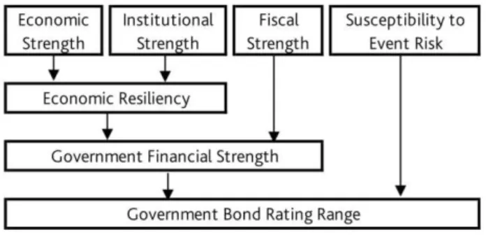
Moody’s rating methodology will now be analysed, to illustrate how the rating methodologies are now more reliant on quantitative inputs. Moody’s Investors Service
(2015) explains how it bases its sovereign credit risk assessment on the “interplay” of
four key factors: economic strength, institutional strength, fiscal strength and
susceptibility to event risk. The following figure show how Moody’s broad factors
interact to ultimately produce a sovereign credit rating.
Figure 1 Key factors affecting Moody's credit risk assessment.
Source:Moody’s Investors Service (2015).
These broad rating factors are subdivided into sub-factors, each with a different weight
towards the broad factor.
5 Often called collateralized debt obligations (CDO).
6 Amstad and Packer (2015) find that ratings can be largely explained by a relatively small set of fewer than
7
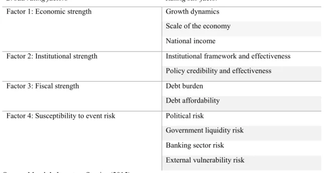
Table I provides further detail about how Moody’s arranges sub-factors into each broad
rating factor.
Table I Identification of Moody's key rating factors and corresponding sub-factors.
Broad rating factors Rating sub-factor7
Factor 1: Economic strength Growth dynamics
Scale of the economy
National income
Factor 2: Institutional strength Institutional framework and effectiveness
Policy credibility and effectiveness
Factor 3: Fiscal strength Debt burden
Debt affordability
Factor 4: Susceptibility to event risk Political risk
Government liquidity risk
Banking sector risk
External vulnerability risk
Source:Moody’s Investors Service (2015).
The transparency achieved by the revision of the Moody’s risk assessment methodology
is illustrated by Cantor (2012), who showed that using the indicators underlying each
factor and their weights as a scorecard, one could predict 70% of Moody’s bond ratings within two notches and explain 67% of the variation in bond ratings.
Al-Sakka and ap Gwilym (2010) associate the growing importance of credit rating
agencies to the increasing number of issuers and debt products, and globalization, but also
to the requirements applied to institutional investors, banks and financial institutions: the
first ones are only allowed to trade debt securities rated by NRSROs, whereas the latter,
stemming from the Basel II Accord, are obliged to use external credit ratings to assess
their credit risks and to determine capital adequacy requirements.
The determinants of sovereign credit ratings are an object of study since the seminal work
of Cantor and Packer (1996), a cross sectional OLS estimation which identified per capita
income, GDP growth, inflation, external debt, level of economic development and default
history as important determinants of sovereign ratings assigned by Moody’s and S&P.
7 Each sub-factor encompasses one or more indicator, like average real GDP growth and volatility, nominal
8
This methodology was also used by Afonso (2003), which also included a logistic and an
exponential transformation of the ratings, in addition to the linear transformation already
used. Mulder and Monfort (2000) and Eliasson (2002) generalized the OLS approach to
panel data, both using a linear transformation of the ratings.
To overcome the limitation of OLS regressions with a linear transformation of the
ratings8, Bissoondoyal-Bheenick (2005) used an ordered probit model for a period of five
years and 95 countries.
Afonso et al. (2008) analysed the determinants of sovereign ratings from the three main
agencies by using a linear regression framework (random effects estimation, pooled OLS
estimation and fixed effects estimation) versus an ordered response framework (ordered
probit9 estimation).
Afonso et al. (2011) confirm that logistic and exponential transformations to ratings
provide little improvement over the linear transformation, not finding evidence of the
so-called “cliff effects” (when investors adjust their portfolio composition to select only
investment grade securities). This work also highlights the difference between short- and
long-term determinants, concluding that GDP per capita, GDP growth, government debt
and budget balance have a short-term impact, whereas government effectiveness, external
debt, foreign reserves and default history influence ratings in the long-run.
Starting with Cantor and Packer (1996) selection of macroeconomic variables, the work
from different authors that followed progressively converged into a subset of
determinants, present in every study here analysed: the level of GDP per capita, real GDP
growth, external debt, the level of public debt and the government budget balance were
found to predominantly explain the rating scale. In line with the results of previous
studies, the recent work of Amstad and Packer (2015), used several explanatory variables
as proxies for fiscal, economic and institutional strength, monetary regime, external
position and default history and also concludes that a small set of factors can largely
explain the rating scale.
8 Ratings represent a qualitative ordinal assessment of a sovereign credit risk, thus the distance between
every two adjacent ratings may not be the same. However, an OLS regression with a linear transformation of the ratings assumes a constant distance between adjacent rating notches.
9 Instead of assuming a rigid shape of the ratings scale, this model estimates the threshold values between
9
3
Methodology
To understand which factors may explain split sovereign ratings and if some of those
factors are considered more relevant by certain agencies, we propose to analyse the
collected dataset using a random-effects probit regression framework.
The source of the information used to create the dependent variables were the rating
changes obtained from Bloomberg for the three main credit rating agencies10. Afterwards,
only long-term sovereign foreign currency ratings were kept, all the other rating changes
were discarded11. For each country and for each year, the last rating change of the year
was selected as that country's year rating. Years without any rating change were filled by
extending the rating of the previous year and rating withdrawals by the rating agencies
were ignored, since the rating given before the withdrawal keeps its relevance for the
markets.
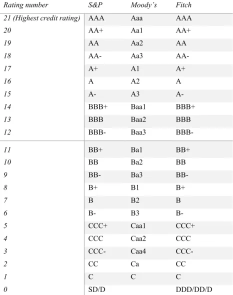
The qualitative rating given by the rating agencies were then converted into a numerical
scale, from 0 to 21, where 21 corresponded to the ‘AAA’ from S&P and Fitch/‘Aaa’ from
Moody's and 0 corresponded to a (selective) default, using the correspondence table from
Hill et al. (2010) shown below. According to Afonso et al. (2012), a logistic or
exponential rating transformation provide little improvement in comparison with the
linear transformation, so the latter was used.
10 Standard & Poor’s, Moody's Investors Service and Fitch Ratings.
11The type of the rating changes downloaded from the Bloomberg platform was “Foreign Currency LT
10
Table II A comparison between rating agencies qualitative scales.
Rating number S&P Moody’s Fitch
21 (Highest credit rating) AAA Aaa AAA
20 AA+ Aa1 AA+
19 AA Aa2 AA
18 AA- Aa3 AA-
17 A+ A1 A+
16 A A2 A
15 A- A3 A-
14 BBB+ Baa1 BBB+
13 BBB Baa2 BBB
12 BBB- Baa3 BBB-
11 BB+ Ba1 BB+
10 BB Ba2 BB
9 BB- Ba3 BB-
8 B+ B1 B+
7 B B2 B
6 B- B3 B-
5 CCC+ Caa1 CCC+
4 CCC Caa2 CCC
3 CCC- Caa4 CCC-
2 CC Ca CC
1 C C C
0 SD/D DDD/DD/D
Source: Hill et al. (2010).
Note: According to S&P Global Ratings (2016), Moody’s Investors Service (2016), Fitch Ratings (2014), we considered a numerical sovereign rating of 12 or above to be an investment-grade rating, whereas a rating below that value would be considered a speculative-grade rating.
Our six dependent variables Diff_UPitSF, Diff_DWitSF, Diff_UPitMF, Diff_DWitMF,
Diff_UPitSM and Diff_DWitSM represent the difference in ratings between the credit rating
agencies considered in this work. Their definition follows:
Diff_UPitSF. It represents the difference between the numeric ratings given by S&P and Fitch, when S&P rating was higher or equal than Fitch’s rating for the
11
Diff_DWitSF. It represents the difference between the numeric ratings given by S&P and Fitch, when S&P rating was lower or equal than Fitch’s rating for the
pair (country i, year t);
Diff_UPitMF. It represents the difference between the numeric ratings given by
Moody’s and Fitch, when Moody’s rating was higher or equal than Fitch’s rating for the pair (country i, year t);
Diff_DWitMF. It represents the difference between the numeric ratings given by
Moody’s and Fitch, when Moody’s rating was lower or equal than Fitch’s rating for the pair (country i, year t);
Diff_UPitSM. It represents the difference between the numeric ratings given by
S&P and Moody’s, when S&P rating was higher or equal than Moody’s rating for the pair (country i, year t);
Diff_DWitSM. It represents the difference between the numeric ratings given by
S&P and Moody’s, when S&P rating was lower or equal than Moody’s rating for the pair (country i, year t)
As an example, let RitX represent the rating from credit rating agency X for the country i
in year t and consider the dependent variable Diff_UPitSM, representing the difference
between S&P and Moody’s ratings: Diff_UPitSM = RitS - RitM, when RitS >= RitM. If
Diff_UPitSM> 0, then S&P considers country i, in time t, more capable of fulfilling its debt
obligations than what Moody’s finds about the capacity of country i to pay its debt. This work reports on the results produced by an ordered and a simple probit models and
as a result, the values of the dependent variables were transformed accordingly: the target
variables of the ordered probit model may assume the values 0, 1 or 2 (as defined by
equation (2)), whereas the target variables of the simple probit model may only assume
the values 0 or 1 (see equation (3)).
3.1 Explanatory variables
The explanatory variables used in this study were selected according to the existing
literature on the determinants of sovereign ratings, where we find previous papers trying
to estimate the predictors of sovereign debt rating notations using both linear (see Cantor
12
(see Afonso et al. (2008), Afonso et al. (2011)). According to these papers, the predictors
which better explain the rating scale are: the level of GDP per capita, real GDP growth,
external debt, government debt and the government budget balance.
In addition to the mentioned predictors12, this work also considered as explanatory
variables the government structural balance, inflation and the default history of a country.
Here follows the list of explanatory variables used in this work (Appendix 1 describes in
more detail each one of these, along with its corresponding source and how each variable
was created):
Budget balance. Overall difference between government revenues and spending. Sequential budget deficits may signal problems with the implemented policies;
Structural balance. By decomposing the budget balance into its cyclical and non-cyclical components, one can better understand the non-cyclical influences on the
budget balance. Changes in the non-cyclical, or structural, component, may be
indicative of discretionary policy adjustments;
Gross debt. Summation of all liabilities that will require payments of interest and/or principal by the government;
Net debt. Net debt is calculated as gross debt minus the financial assets a government holds;
GDP growth rate. Annual growth rate of the Gross Domestic Product. A higher
value strengths the government ability to pay its debt;
GDP per capita. Also called per capita income, measures the average income per person in a country;
Inflation. Annual increase of average consumer prices, over a period of time. It helps governments by reducing the real stock of outstanding debt in domestic
currency, but a consistent high value is associated with macroeconomic
imbalances;
External debt. Also called foreign debt, represents the total debt a country (its
government, corporations and citizens) owes to foreign creditors. It does not
include contingent liabilities;
12 With regard to the government debt, this work analysed both gross and net government debt as separate
13
Default-in-the-last-year/2-years/5-years/10-years. These variables represent a default in the last year, two, five or ten years. The definition of default by Beers
and Mavalwalla (2016) here used is consistent with the literature on sovereign
defaults and considers that “a default has occurred when debt service is not paid
on the due date, payments are not made within the time frame specified under a
guarantee or, absent an outright payment default, creditors face material economic
losses on the sovereign debt they hold”.
3.2 Probit regression framework
In this work we used both a random effects ordered probit and simple probit panel model,
similar to what Afonso et al. (2011) used to identify the determinants of sovereign debt
credit ratings and what Al-Sakka and ap Gwilym (2010) used to analyse the impact of
split ratings on sovereign rating changes. According to Afonso et al. (2011), the ordered
and simple probit random-effects estimations consider the existence of an additional
cross-country error term and therefore yield better results using panel data when
compared with linear regression methods or fixed-effects probit estimations.
Our approach considers the discrete, ordinal nature of rating differences between credit
rating agencies. The negative and positive rating differences for each pair of agencies was
analysed separately due to expected disparate behaviour, comparable to what Al-Sakka
and ap Gwilym (2010) expected with rating migrations.
Consider our probit regression setting, when we are regressing Diff_UPitSM as the
dependent variable (in this case, all observations have the rating from S&P higher or equal
than the rating from Moody’s). If the resulting coefficient of an explanatory variable, say,
real GDP growth, is positive and significant, we conclude that an increase in real GDP
growth will contribute to a bigger difference between S&P and Moody’s ratings13. In a
similar way, if the coefficient of the level of public debt is negative, we may conclude
that an increase in the level of public debt, will contribute to a smaller difference between
the ratings given by S&P and Moody’s14.
13 This could be interpreted as an increase in real GDP growth contributing to a higher S&P rating or a
lower Moody’s rating.
14 And in this case this could be interpreted as an increase in the level of public debt contributing to a lower
14
Our probit specification is defined as follows, and the value of our 𝑦𝑖𝑡 dependent variable depends on whether we are considering the ordered probit or the simple probit approach:
𝑦𝑖𝑡 = 𝛽1𝐺𝑜𝑣𝐷𝑒𝑏𝑡𝑃𝑟𝑜𝑥𝑦𝑖𝑡+ 𝛽2𝑁𝐺𝐷𝑃_𝑅𝑃𝐶𝐻𝑖𝑡+ 𝛽3𝑁𝐺𝐷𝑃𝐷𝑃𝐶𝑖𝑡
+ 𝛽4𝑃𝐶𝑃𝐼𝑃𝐶𝐻𝑖𝑡+ 𝛽5𝐸𝑥𝑡𝐷𝑒𝑏𝑡𝑃𝑒𝑟𝑐𝐺𝑁𝐼𝑖𝑡+ 𝛾𝐷𝑒𝑓𝑎𝑢𝑙𝑡𝑍𝑖𝑡
+ 𝜀𝑖𝑡; 𝜀𝑖𝑡~𝑁(0, 1)
𝑖 = 1, … 𝐶 (𝑛𝑜. 𝑜𝑓 𝑐𝑜𝑢𝑛𝑡𝑟𝑖𝑒𝑠), 𝑡 = 1, … 𝑌 (𝑛𝑜. 𝑜𝑓 𝑦𝑒𝑎𝑟𝑠)
(1)
Where 𝑦𝑖𝑡 is an ordinal variable equal to either Diff_UPitAB or Diff_DWitAB.
On our ordered probit model, Diff_UPitAB (Diff_DWitAB) = 1 or 2 if the rating from agency
A is higher (lower) than the rating from agency B by one or more-than-one-notch,
respectively, for sovereign i in year t, and 0 otherwise.
On our simple probit model, Diff_UPitAB (Diff_DWitAB) = 1 if the rating from agency A is
higher (lower) than the rating from agency B by one or more notches, for sovereign i in
year t, and 0 otherwise.
𝐺𝑜𝑣𝐷𝑒𝑏𝑡𝑃𝑟𝑜𝑥𝑦𝑖𝑡 may assume the variation value of the budget balance, gross debt, net
debt or structural balance of country i in year t, depending on the chosen specification15.
𝑁𝐺𝐷𝑃_𝑅𝑃𝐶𝐻𝑖𝑡 is the growth rate of GDP for country i in year t.
𝑁𝐺𝐷𝑃𝐷𝑃𝐶𝑖𝑡 is the GDP per capita variation for country i in year t.
𝑃𝐶𝑃𝐼𝑃𝐶𝐻𝑖𝑡 is the inflation percentage change for country i in year t.
𝐸𝑥𝑡𝐷𝑒𝑏𝑡𝑃𝑒𝑟𝑐𝐺𝑁𝐼𝑖𝑡 is the external debt variation for country i in year t.
𝐷𝑒𝑓𝑎𝑢𝑙𝑡𝑍𝑖𝑡 is a dummy variable taking the value of 1 if the country i in year t had
defaulted in the last Z years, and 0 otherwise.
In the scope of the ordered probit framework, our six dependent variables were defined
as to only have values of 1, 2 or 0, representing a rating gap of 1-notch, 2-or-more-notches
or the inexistence of a rating gap, respectively. Equation 2 represents how the target
variables were created:
𝐷𝑖𝑓𝑓𝛿
𝑖𝑡𝛼𝛽 =
{
1, 𝑖𝑓 |𝑅𝑖𝑡𝛼− 𝑅𝑖𝑡𝛽| = 1
2, 𝑖𝑓 |𝑅𝑖𝑡𝛼− 𝑅 𝑖𝑡𝛽| ≥ 2
0, 𝑜𝑡ℎ𝑒𝑟𝑤𝑖𝑠𝑒
, 𝛿 = {𝑈𝑃, 𝑖𝑓 𝑅𝑖𝑡𝛼 ≥ 𝑅𝑖𝑡
𝛽
𝐷𝑊, 𝑖𝑓 𝑅𝑖𝑡𝛼 ≤ 𝑅 𝑖𝑡𝛽
𝑤ℎ𝑒𝑟𝑒 𝛼 𝑎𝑛𝑑 𝛽 ∈ {𝑆𝐹, 𝑀𝐹, 𝑆𝑀}.
(2)
15 All specifications are defined on Table III.
15
A simple probit regression was also run afterwards, and so the dependent variables were
defined accordingly, by only assuming values of 0 or 1, as one may see in the following
equation:
𝐷𝑖𝑓𝑓𝛿
𝑖𝑡
𝛼𝛽 = {1, 𝑖𝑓 |𝑅𝑖𝑡
𝛼− 𝑅 𝑖𝑡𝛽| ≥ 1
0, 𝑜𝑡ℎ𝑒𝑟𝑤𝑖𝑠𝑒 , 𝛿 = {
𝑈𝑃, 𝑖𝑓 𝑅𝑖𝑡𝛼 ≥ 𝑅𝑖𝑡𝛽
𝐷𝑊, 𝑖𝑓 𝑅𝑖𝑡𝛼 ≤ 𝑅𝑖𝑡𝛽
𝑤ℎ𝑒𝑟𝑒 𝛼 𝑎𝑛𝑑 𝛽 ∈ {𝑆𝐹, 𝑀𝐹, 𝑆𝑀}.
(3)
This leads to, in the context of the simple probit regression, our dependent variables
having a value of 1 if there is a rating difference of 1-notch or higher and a value of 0 if
the ratings from the considered pair of agencies are equivalent in our numerical rating
scale.
Four different specifications of predicting variables were considered to overcome the
correlation between some of the variables. Within each specification, the four different
default dummies were combined. The composition of each specification can be seen on
following table.
Table III Composition of the specifications used in this work, combining the different predicting variables. These specifications were used with both the ordered probit and the simple probit models.
Specification Predicting variables
Budget
balance BudgetBal_NGDP, NGDP_RPCH, NGDPDPC, PCPIPCH, ExtDebtPercGNI, DefaultLastY BudgetBal_NGDP, NGDP_RPCH, NGDPDPC, PCPIPCH, ExtDebtPercGNI, DefaultLast2Y
BudgetBal_NGDP, NGDP_RPCH, NGDPDPC, PCPIPCH, ExtDebtPercGNI, DefaultLast5Y
BudgetBal_NGDP, NGDP_RPCH, NGDPDPC, PCPIPCH, ExtDebtPercGNI, DefaultLast10Y
Gross debt GGXWDG_NGDP, NGDP_RPCH, NGDPDPC, PCPIPCH, ExtDebtPercGNI, DefaultLastY
GGXWDG_NGDP, NGDP_RPCH, NGDPDPC, PCPIPCH, ExtDebtPercGNI, DefaultLast2Y
GGXWDG_NGDP, NGDP_RPCH, NGDPDPC, PCPIPCH, ExtDebtPercGNI, DefaultLast5Y
GGXWDG_NGDP, NGDP_RPCH, NGDPDPC, PCPIPCH, ExtDebtPercGNI, DefaultLast10Y
Net debt GGXWDN_NGDP, NGDP_RPCH, NGDPDPC, PCPIPCH, ExtDebtPercGNI, DefaultLastY
GGXWDN_NGDP, NGDP_RPCH, NGDPDPC, PCPIPCH, ExtDebtPercGNI, DefaultLast2Y
GGXWDN_NGDP, NGDP_RPCH, NGDPDPC, PCPIPCH, ExtDebtPercGNI, DefaultLast5Y
16
Structural balance
GGSB_NPGDP, NGDP_RPCH, NGDPDPC, PCPIPCH, ExtDebtPercGNI, DefaultLastY
GGSB_NPGDP, NGDP_RPCH, NGDPDPC, PCPIPCH, ExtDebtPercGNI, DefaultLast2Y
GGSB_NPGDP, NGDP_RPCH, NGDPDPC, PCPIPCH, ExtDebtPercGNI, DefaultLast5Y
GGSB_NPGDP, NGDP_RPCH, NGDPDPC, PCPIPCH, ExtDebtPercGNI, DefaultLast10Y
4
Empirical analysis
4.1 Data
With regards to the dependent variables, all the sovereign rating changes16 were
downloaded from Bloomberg and converted into a numerical scale using Table II.
Afterwards, we created six dependent variables (described in section 3), two variables for
each rating agency pair, with the value of each variable reflecting the numerical rating
difference between the ratings given by those specific agencies (comparable to what
Livingston et al. (2008) did with the split rated issues).
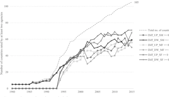
Figure 2 Total number of countries rated by at least two credit rating agencies, and number of countries rated by each pair of the rating agencies considered in this work.
Source: rating agencies and own calculations.
The initial objective of this work was to study rating differences from 1970 onwards.
However, and due to the inexistence of both macroeconomic values for many countries
16 We used the sovereign issuer ratings for foreign currency denominated debt.
105
0 20 40 60 80 100
1980 1985 1990 1995 2000 2005 2010 2015
Nu
m
b
er
o
f
co
u
n
tr
ies
rated
b
y
at
least
tw
o
ag
en
cies
17
on those early years and ratings from at least two of the three selected agencies, our
observations happened to comprehend only the period between 1980 and 2015. As Figure
2 illustrates, we only have observations with a rating from Fitch from 1994 onwards.
From 1990 and until 2000, we observe a bigger increase in the number or countries rated
by at least two agencies, whereas from 2000 onwards the pace of this increase slowed,
ending with 105 countries in our dataset with ratings from at least two of the main rating
agencies.
The distribution of the sovereign ratings on our dataset (seen in Figure 3) show that S&P
is the agency which assigns more countries a rating of ‘AA-’ or above, and that the great
majority of our observations are equal or above ‘B-’. A higher degree of agreement on the top of the rating scale may explain the number of observations which had a rating of
‘AAA’ from all three agencies.
Figure 3 Distribution of the sovereign ratings composing our dataset. The time periods are 1980
to 2015 for S&P and Moody’s and 1994 to 2015 for Fitch.
Source: rating agencies and own calculations.
In Table IV one may find some of the countries analysed in the scope of this work. The
higher number of countries added to our observations in 1995 and 2000 reflect the
behaviour of the total number of countries already seen on Figure 3.
Our independent variables were obtained from datasets from the IMF (World Economic
Outlook), World Bank (World Development Indicators), Bank of Canada (Database of 0
50 100 150 200 250 300 350 400
0 1 2 3 4 5 6 7 8 9 10 11 12 13 14 15 16 17 18 19 20 21
N
u
m
b
er
o
f
an
n
u
al
o
b
se
rv
ati
o
n
s
18
Sovereign Defaults) and from the Quarterly External Debt Statistics dataset developed in
collaboration between the World Bank and the IMF. Details on how those variables were
created can be found in Table A1-1.
Table IV Countries in our full dataset which in the previous period did not have ratings from two or more of the three main agencies.
Source: rating agencies and own calculations.
4.2 Ordered probit panel results
This section will dissect the results generated by the ordered probit panel regression for
the rating differences between every pair of rating agencies. We first considered the full
dataset in our regressions. Then, our dataset was split into two subsets depending on the
value of the average rating from each pair of rating agencies: a set with investment-grade
average ratings and a set with speculative-grade average ratings. We ran the ordered
probit regressions with the three datasets, for each of the four specifications of predicting
variables.
1980 1985 1990 1995 2000 2005 2010 2015
Australia Denmark Argentina Barbados Bahrain Albania Angola
Austria Finland Belgium Belize Cameroon Azerbaijan Armenia
United Kingdom Ireland Brazil Bulgaria Dominican Republic Belarus Côte d'Ivoire
Norway Malaysia Canada Costa Rica El Salvador Bosnia and Herzegovina Ethiopia
Sweden New Zealand Chile Croatia Ghana Fiji Honduras
Spain China Ecuador Guatemala Gabon Iraq
Thailand Colombia Egypt Mali Georgia Namibia
Czech Republic Estonia Mongolia Jordan Paraguay
France India Mozambique Kenya Rwanda
Germany Jamaica Saudi Arabia Libya Senegal
Greece Kazakhstan Serbia Nigeria Zambia
Hungary Korea (Republic of) Sri Lanka Seychelles
Iceland Kuwait Ukraine Uganda
Indonesia Lebanon Viet Nam United Arab Emirates
Israel Morocco
Italy Oman
Japan Panama
Luxembourg Papua New Guinea
Mexico Peru Netherlands Qatar
Pakistan Romania
Philippines Russian Federation Poland Slovenia
Portugal Trinidad and Tobago
South Africa Tunisia
Switzerland Turkey
United States
19
4.2.1 Full sample
We started by running the ordered probit regression with the full dataset. This dataset was
composed by more than 850 observations for each dependent variable, comprised a period
of at least 22 years (36 years only for the rating agency pair S&P and Moody’s) and 69
or more countries. More than 65% of our observations for each of our target variables had
no rating difference, whereas a rating difference of 1-notch was found at least in 19% of
the observations. A rating difference of two or more notches can only be found 3.5%17 of
the times when analysing comparable ratings from S&P and Fitch; on the other hand,
9%18of the observations about the rating differences between S&P and Moody’s have a
2-notch rating difference. This shows how S&P and Moody’s disagree more when
compared with the other rating agency pairs. Table V summarizes the full dataset.
Table V Summary of the full dataset, divided by the six target variables.
Diff_UPitSF Diff_DWitSF Diff_UPitMF Diff_DWitMF Diff_UPitSM Diff_DWitSM
No. of countries 87 87 70 69 82 82
No. of years 22 22 22 22 36 36
First and last year 1994-2015 1994-2015 1994-2015 1994-2015 1980-2015 1980-2015
No. of observations 1149 1194 903 851 1103 1165
Observations with:
Rating difference = 0 898 (78%) 898 (75%) 606 (67%) 606 (71%) 764 (69%) 764 (66%)
Rating difference = 1 221 (19%) 248 (21%) 223 (25%) 187 (22%) 247 (22%) 286 (25%)
Rating difference = 2 30 (3%) 48 (4%) 74 (8%) 58 (7%) 92 (8%) 115 (10%)
No. of observations with a value:
GDP per capita 1149 (100%)
1194 (100%) 903 (100%) 851 (100%) 1103 (100%)
1165 (100%)
Real GDP growth rate 1148 (100%)
1194 (100%) 903 (100%) 851 (100%) 1103 (100%)
1165 (100%)
17 This value was obtained by calculating the average of the percentages of a rating difference of two or
more notches between S&P and Fitch, when the first gave a higher rating than the latter (Diff_UPitSF) and
when the first gave a lower rating than the latter (Diff_DWitSF).
18 This value was obtained by calculating the average of the percentages of a rating difference of two or
more notches between S&P and Moody’s, when the first gave a higher rating than the latter (Diff_UPitSM)
20
External debt 841 (73%) 897 (75%) 685 (76%) 648 (76%) 701 (64%) 808 (69%)
Gov. gross debt 1096 (95%)
1135 (95%) 865 (96%) 807 (95%) 1018 (92%)
1065 (91%)
Gov. net debt 1046 (91%)
1085 (91%) 822 (91%) 770 (90%) 954 (86%) 1004 (86%)
Budget balance 1112 (97%)
1153 (97%) 877 (97%) 824 (97%) 1057 (96%)
1104 (95%)
Structural balance 1064 (93%)
1100 (92%) 842 (93%) 774 (91%) 970 (88%) 1028 (88%)
Inflation 1147
(100%)
1191 (100%) 901 (100%) 848 (100%) 1100 (100%)
1160 (100%)
Default in the:
Last year 312 (27%) 321 (27%) 164 (18%) 211 (25%) 268 (24%) 258 (22%)
Last two years 349 (30%) 363 (30%) 190 (21%) 247 (29%) 311 (28%) 297 (25%)
Last five years 419 (36%) 446 (37%) 248 (27%) 313 (37%) 379 (34%) 375 (32%)
Last ten years 522 (45%) 539 (45%) 331 (37%) 366 (43%) 448 (41%) 454 (39%)
Source: rating agencies and own calculations.
Running the ordered probit regression for the full dataset, when the ratings from S&P are
higher or equal to Fitch own ratings (Diff_UPitSF dependent variable), we get significant
values for both budget balance and net debt variables. When budget balance increases,
we expect the rating difference to decrease. For the net debt predicting variable the
opposite occurs: when its value increases, the rating difference increases as well.
With regard to the Diff_DWitSF dependent variable (ratings from S&P being lower or equal
to Fitch ratings), GDP per capita, external debt and the dummy default-in-the-last-5-years
variables have statistically significant coefficients on all specifications. One can then
conclude that if GDP per capita or external debt decrease, the rating difference between
those two rating agencies increases. The coefficients of the dummy
default-in-the-last-5-years are also significant (and positive), showing that a default in the last five default-in-the-last-5-years
increases the rating difference between S&P and Fitch in this case.
Analysing the rating difference between Moody's and Fitch, when the rating given by
Moody's is higher than Fitch’s rating (Diff_UPitMF), we find significant values for two
dependent variables, GDP growth (negative coefficient on two specifications) and
external debt level (positive coefficients on all specifications). These results show that
21
smaller, whereas when the level of external debt increases, the gap between these two
agencies increases.
When Moody's rating is lower than the rating from Fitch (Diff_DWitMF), we find that the
dummy variable representing a default in the last five years has a positive coefficient in
all specifications. For this reason, if a default in the last five years occurred, the rating
difference in this setting between Moody's and Fitch increases as well.
The variables gross debt and net debt also have significant values of opposite signs: the
gross debt contributes negatively for the rating difference, reducing the rating difference
when its value increases, while the net debt has positive coefficients, so its increase is
expected to positively influence the magnitude of the rating difference. We need to better
understand the opposite signs of these two variables, since they should be correlated to a
certain degree. The separate regressions of the investment and speculative ratings may
shed some light into this topic.
The results from regressing our dependent variable Diff_UPitSM (when the S&P rating is
higher than Moody's rating), display significant results only for the dummy default
variables. The dummy default-in-the-last-2-years has positive coefficients on all
specifications, meaning that if a country defaults in the last two years, the rating gap
between S&P and Moody's will grow.
The results from regressing the last set of specifications, when the rating from S&P is
lower than the rating from Moody's (Diff_UPitSM dependent variable), show that the
budget balance, gross debt, GDP growth and GDP per capita variables all contribute to
the rating difference in question. Those first three variables have statistically significant
and positive coefficients, meaning that when one of those variables increase, the rating
difference between S&P and Moody's (Diff_UPitSM) will increase as well. The coefficient
of the GDP per capita variable is negative, so when its value increases, the rating gap
between S&P and Moody's becomes smaller.
The main results of running the ordered probit regressions with our full dataset are shown
in the table below, and the full results may be seen on Appendix 2:
Table VI Summary of the regressions of the ordered probit full dataset.
Significant variables Marginal Effect Rating difference = 1
22
Diff_UPitSF (-) Budget balance (4/4)
(+) Net debt (4/4)
-0.001%
0.0004%
-0.00008%
0.00003%
Diff_DWitSF (-) GDP per capita (16/16)
(-) External debt (16/16)
(+) Default last 1Y (1/4)
(+) Default last 2Y (1/4)
(+) Default last 5Y (4/4)
-0.3% -0.1% 12.3% 11.5% 10.1%-10.5% -0.03% -0.01% 1.9% 1.7% 1.3%-1.5%
Diff_UPitMF (-) GDP growth (9/16)
(+) External debt (16/16)
-0.9%--1%
0.1%-0.2%
-0.2%
0.03%-0.04%
Diff_DWitMF (-) Gross debt (2/4)
(+) Net debt (4/4)
(+) Default last 2Y (3/4)
(+) Default last 5Y (4/4)
-0.2% 0.0003% 10.8%-11.4% 11.3%-12.1% -0.05%--0.06% 0.00007% 2.9%-3% 3%-3.2%
Diff_UPitSM (+) Default last Y (1/4)
(+) Default last 2Y (4/4)
(+) Default last 5Y (1/4)
(+) Default last 10Y (1/4)
6.1% 8.1%-11.4% 12.9% 12.7% 2% 2.7%-3.5% 3.9% 3.6%
Diff_DWitSM (+) Budget balance (4/4)
(+) Gross debt (4/4)
(+) GDP growth (4/16)
(-) GDP per capita (8/16)
0.005% 0.2% 0.8% -0.3% 0.002% 0.07% 0.2% -0.08%--0.09%
Note: Coefficient signs and number of significant regressions (besides the total number of run regressions) in parenthesis.
4.2.2 Differentiation between investment and speculative ratings
We will now report the ordered probit regression results when the observations used as
input were divided into two subsets, depending on the value of the average rating given
by the rating agency pair. The observations with a numeric average rating of 12 or more19
were grouped in the investment-grade subset, whereas those with a numeric rating less
than 12 were grouped in the speculative-grade subset.
4.2.2.1 Investment-grade subset
This section will analyse the results from the ordered probit regression when considering
only observations with an investment-grade average rating. When compared with the full
dataset, the investment-grade dataset had observations for a smaller number of countries,
23
between 49 and 57 different countries. The adopted criteria of considering only those
observations with an investment-grade average rating reduced as expected the number of
observations for each target variable (all target variables had less than 800 observations).
It’s important to note a higher percentage of observations with the same rating (when compared with the full dataset) from each rating agency in this setting, reflecting a greater
coherence between the studied rating agencies when considering investment-grade
sovereigns. This may be explained by Livingston et al. (2007) opaqueness idea which
associates bond split ratings with the opaqueness of the issuer. In this case,
investment-grade sovereign issuers disclose more detailed information, allowing rating agencies to
better evaluate their ability to service debt and therefore rating agencies will agree more
often about a country’s rating in this context, leading to a higher percentage of observations with a rating difference of 0. Table VII summarizes the dataset used in this
section.
Our regression, when the S&P rating is higher than the rating from Fitch (Diff_UPitSF
dependent variable), only yield significant results for one of the specifications (only one
of the regressions show the budget balance variable as significant). This specification
shows a positive correlation between government net debt and the observed rating
difference, when the ratings from S&P and Fitch are investment-grade.
When the rating from S&P is lower than the one from Fitch (Diff_DWitSF), the obtained
results for all specifications show a negative correlation between GDP per capita and the
rating difference. This means that when GDP per capita increases, the rating difference is
reduced. Only one of the regressions in this setting shows a significant and positive
default dummy variable (the last year one).
Table VII Summary of the investment-grade dataset, divided by the six target variables.
Diff_UPitSF Diff_DWitSF Diff_UPitMF Diff_DWitMF Diff_UPitSM Diff_DWitSM
No. of countries 57 56 50 49 52 52
No. of years 22 22 22 22 36 36
First and last year 1994-2015 1994-2015 1994-2015 1994-2015 1980-2015 1980-2015
No. of observations 773 759 665 555 746 795
24
Rating difference = 0 634 (82%) 634 (84%) 466 (70%) 466 (84%) 568 (76%) 568 (71%)
Rating difference = 1 124 (16%) 112 (15%) 145 (22%) 64 (12%) 124 (17%) 157 (20%)
Rating difference = 2 15 (2%) 13 (2%) 54 (8%) 25 (5%) 54 (7%) 70 (9%)
No. of observations with a value:
GDP per capita 773 (100%)
759 (100%) 665 (100%) 555 (100%) 746 (100%) 795 (100%)
Real GDP growth rate 772 (100%)
759 (100%) 665 (100%) 555 (100%) 746 (100%) 795 (100%)
External debt 491 (64%) 491 (65%) 462 (69%) 370 (67%) 378 (51%) 472 (59%)
Gov. gross debt 750 (97%) 735 (97%) 655 (99%) 544 (98%) 693 (93%) 734 (92%)
Gov. net debt 700 (91%) 675 (89%) 605 (91%) 499 (90%) 641 (86%) 673 (85%)
Budget balance 753 (97%) 738 (97%) 658 (99%) 547 (99%) 717 (96%) 760 (96%)
Structural balance 727 (94%) 713 (94%) 643 (97%) 528 (95%) 661 (89%) 709 (89%)
Inflation 772 (100%)
759 (100%) 665 (100%) 555 (100%) 746 (100%) 795 (100%)
Default in the:
Last year 74 (10%) 66 (9%) 46 (7%) 42 (8%) 56 (8%) 56 (7%)
Last two years 87 (11%) 76 (10%) 55 (8%) 52 (9%) 65 (9%) 63 (8%)
Last five years 117 (15%) 104 (14%) 77 (12%) 73 (13%) 88 (12%) 87 (11%)
Last ten years 177 (23%) 153 (20%) 124 (19%) 104 (19%) 127 (17%) 130 (16%)
Source: rating agencies and own calculations.
The regressions of our dependent variable Diff_UPitMF (rating from Moody's higher than
the one from Fitch, with the average classified as investment-grade) showed a positive
and negative correlation between the rating difference and, respectively, GDP per capita
and inflation. In this case, when GDP per capita increases, the rating gap increases,
whereas with an inflation increase, the rating divergence between those two agencies will
diminish.
While analysing the results when we regress the Diff_DWitMF (rating difference when the
25
regressions showing a significant coefficient for the government gross debt predicting
variable.
All the regressions of the Diff_UPitSM target variable (rating difference when the rating
from S&P is higher than the rating from Moody's, and, on average, both ratings are
investment-grade) show a significant negative correlation between external debt and the
rating difference, leading to a smaller rating difference when the level of external debt
rises.
The last dependent variable, Diff_DWitSM, yield significant results when regressed against
our predicting variables: both budget balance and government gross debt have significant
positive coefficients20, meaning that an increase of those variables will lead to an increase
in the rating difference between S&P and Moody's, when the rating of the first is lower
than the rating of the latter.
The GDP growth predicting variable also has significant positive coefficients on two of
the four regressed specifications, showing an effect on the rating difference similar to the
described effect of the budget balance and government gross debt on the rating gap. We
also observe statistically significant and negative coefficients for two of the default
dummy variables21, meaning that the existence of a default in the last year or two will
contribute to a smaller rating difference between S&P and Moody's in this case.
The following table summarizes the significant results obtained when regressing the
investment-grade subset (the full results may be consulted in Appendix 3):
Table VIII Summary of the regressions of the ordered probit investment-grade subset.
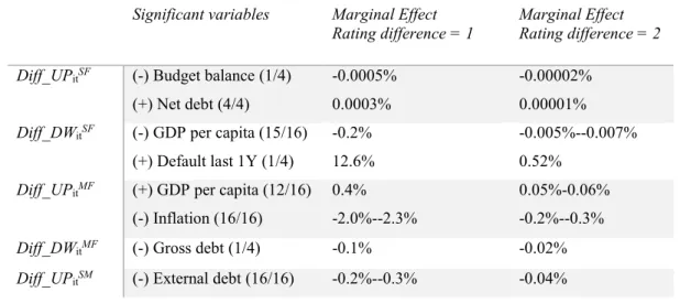
Significant variables Marginal Effect Rating difference = 1
Marginal Effect Rating difference = 2
Diff_UPitSF (-) Budget balance (1/4)
(+) Net debt (4/4)
-0.0005%
0.0003%
-0.00002%
0.00001%
Diff_DWitSF (-) GDP per capita (15/16)
(+) Default last 1Y (1/4)
-0.2%
12.6%
-0.005%--0.007%
0.52%
Diff_UPitMF (+) GDP per capita (12/16)
(-) Inflation (16/16)
0.4%
-2.0%--2.3%
0.05%-0.06%
-0.2%--0.3%
Diff_DWitMF (-) Gross debt (1/4) -0.1% -0.02%
Diff_UPitSM (-) External debt (16/16) -0.2%--0.3% -0.04%
20 With a significance level of 1% for all the relevant regressions.
26
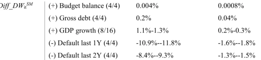
Diff_DWitSM (+) Budget balance (4/4)
(+) Gross debt (4/4)
(+) GDP growth (8/16)
(-) Default last 1Y (4/4)
(-) Default last 2Y (4/4)
0.004%
0.2%
1.1%-1.3%
-10.9%--11.8%
-8.4%--9.3%
0.0008%
0.04%
0.2%-0.3%
-1.6%--1.8%
-1.3%--1.5%
Note: Coefficient signs and number of significant regressions (besides the total number of run regressions) in parenthesis.
4.2.2.2 Speculative-grade subset
Lastly, the results from the ordered probit regression using the same specifications will
be analysed, but this time using a subset of the full dataset composed only by observations
with a speculative-grade average rating. This speculative-grade subset has observations
for at least 38 countries22 and comprehends the period from 1992 to 2015. We have much
less observations (between 238 and 435 observations) for the speculative-grade dataset
when compared with the investment-grade and full datasets. By analysing Table IX we
can observe that the same rating can only be found on 70% of the observations for the
Diff_UPitSF target variable, reaching as low as 47% of the observations for the rating
differences between Moody’s and Fitch, when the rating from the first is lower than the
rating from the latter. This fact reflects how opaque speculative-grade sovereigns are and
how difficult is for credit rating agencies to assess the real capability of these sovereigns
to service their debt. This lack of transparency leads to the information available to rating
agencies having poor quality and increases the probability of a split rating (Al-Sakka and
ap Gwilym (2010)).
The following table summarizes the dataset used in this section.
Table IX Summary of the speculative-grade dataset, divided by the six target variables.
Diff_UPitSF Diff_DWitSF Diff_UPitMF Diff_DWitMF Diff_UPitSM Diff_DWitSM
No. of countries 54 53 42 38 50 51
No. of years 22 22 22 22 23 24
First and last year 1994-2015 1994-2015 1994-2015 1994-2015 1993-2015 1992-2015
No. of observations 376 435 238 296 357 370
Observations with:
22 For the Diff_DW
itMFtarget variable; the remaining target variables include observations for more than 50
27
Rating difference = 0 264 (70%) 264 (61%) 140 (59%) 140 (47%) 196 (55%) 196 (53%)
Rating difference = 1 97 (26%) 136 (31%) 78 (33%) 123 (42%) 123 (34%) 129 (35%)
Rating difference = 2 15 (4%) 35 (8%) 20 (8%) 33 (11%) 38 (11%) 45 (12%)
No. of observations with a value:
GDP per capita 376 (100%)
435 (100%) 238 (100%) 296 (100%) 357 (100%)
370 (100%)
Real GDP growth rate
376 (100%)
435 (100%) 238 (100%) 296 (100%) 357 (100%)
370 (100%)
External debt 350 (93%) 406 (93%) 223 (94%) 278 (94%) 323 (90%) 336 (91%)
Gov. gross debt 346 (92%) 400 (92%) 210 (88%) 263 (89%) 325 (91%) 331 (89%)
Gov. net debt 346 (92%) 410 (94%) 217 (91%) 271 (92%) 313 (88%) 331 (89%)
Budget balance 359 (95%) 415 (95%) 219 (92%) 277 (94%) 340 (95%) 344 (93%)
Structural balance 337 (90%) 387 (89%) 199 (84%) 246 (83%) 309 (87%) 319 (86%)
Inflation 375 (100%)
432 (99%) 236 (99%) 293 (99%) 354 (99%) 365 (99%)
Default in the:
Last year 238 (63%) 255 (59%) 118 (50%) 169 (57%) 212 (59%) 202 (55%)
Last two years 262 (70%) 287 (66%) 135 (57%) 195 (66%) 246 (69%) 234 (63%)
Last five years 302 (80%) 342 (79%) 171 (72%) 240 (81%) 291 (82%) 288 (78%)
Last ten years 345 (92%) 986 (89%) 207 (87%) 262 (89%) 321 (90%) 324 (88%)
Source: rating agencies and own calculations.
The first regressions have the Diff_UPitSF as the dependent variable and produce
significant results for the budget balance and government net debt variables (only one of
the regressions with this target variable show the dummy default-in-the-last-5-years
variable as significant). The budget balance coefficient is negative, leading to a smaller
rating difference between S&P and Fitch when the budget balance grows. Government
net debt has the opposite effect on the described rating difference: when it increases, the
rating disparity between those two agencies increases as well.
With regards to the obtained results when regressing the Diff_DWitSF variable, it is
possible to observe that government net debt, GDP growth, external debt level and the
28
between S&P and Fitch, when the rating from the first is lower than the rating from the
latter. The government net debt variable has a positive coefficient, increasing the rating
difference when its value increases. The remaining significant variables (GDP growth,
external debt level and the dummy default variable) have negative coefficients, so when
their value increases (or becomes one, in the case of the dummy variable), the rating
difference between S&P and Fitch shrinks.
Only one of the specifications yield significant results when regressing the Diff_UPitMF
variable (rating difference between Moody's and Fitch, with a higher rating from the first
agency). External debt has positive and significant coefficients on two of the regressions,
therefore when its value increases, the analysed rating difference increases as well. Two
of the four dummy default variables (default in the last year and in the last five years)
have significant negative coefficients, thus when a default happened in the last year or in
the last five years, the rating difference will get smaller.
The regression of the Diff_DWitMF target variable against the different specifications of
predicting variables highlights the effect of government gross debt and inflation on the
rating difference between Moody's and Fitch, when the first is lower than the latter (the
dummy default-in-the-last-10-years variable only yielded significant and negative results
for one of the regressions). Both gross debt and inflation contribute negatively to the
rating gap, therefore, the rating difference will shrink if one of those variables increases.
Table X Summary of the regressions of the ordered probit speculative-grade subset.
Significant variables (Coefficient sign)
Marginal Effect Rating difference = 1
Marginal Effect Rating difference = 2
Diff_UPitSF (-) Budget balance (4/4)
(+) Net debt (4/4)
(-) Default last 5Y (1/4)
-0.002%
0.2%
-17.3%
-0.0001%
0.01%
-2.8%
Diff_DWitSF (+) Net debt (4/4)
(-) GDP growth (15/16)
(-) External debt (15/16)
(-) Default last 10Y (3/4)
0.2%
-1.2%--1.3%
-0.1%--0.2%
-11.7%--12.7%
0.04%
-0.3%--1%
-0.03%--0.07%
-3.8%--5.9%
Diff_UPitMF (+) External debt (2/16)
(-) Default last Y (1/4)
(-) Default last 5Y (1/4)
0.2%
-13.2%
-20.4%
0.05%
-3.1%
-5.6%
29
(-) Inflation (4/4)
(-) Default last 10Y (1/4)
-0.3%
-11%
-0.1%--0.2%
-10.2%
Diff_UPitSM (-) Net debt (4/4) -0.2% -0.06%
Diff_DWitSM (+) Budget balance (3/4)
(-) GDP per capita (12/16)
(-) External debt (4/16)
0.007%
-0.4%--0.5%
-0.2%
0.001%
-0.08%--0.1%
-0.05%
Note: Coefficient signs and number of significant regressions (besides the total number of run regressions) in parenthesis.
All the ordered probit regressions run with Diff_UPitSM as the dependent variable show
that the government net debt contributes negatively to the rating difference, when the
S&P rating is higher than the rating from Moody's. As a result, when the government net
debt increases, the rating gap between S&P and Moody's shrinks.
The results from regressing the Diff_DWitSM target variable show a positive and a negative
correlation between the rating difference (when the rating from S&P is lower than the one
from Moody's) and, respectively, the budget balance on one hand, and GDP per capita
and external debt on the other hand. For this reason, when the budget balance increases,
the considered rating gap increases; whereas, when GDP per capita or external debt
increase, the same rating gap decreases.
Table X summarizes the significant results obtained when regressing the
speculative-grade subset (Appendix 4 contains the full results).
4.3 Simple probit panel results
When regressing our target variables (Diff_UPitSF, Diff_DWitSF, Diff_UPitMF,
Diff_DWitMF, Diff_UPitSM and Diff_DWitSM) with the ordered probit framework, we found
that only 3% to 10% of our observations had a rating gap of 2-notches or higher (this can
be seen on the summary of Table V). Therefore, we decided to run a simple probit
regression for the same observations subsets already used: we first considered the full
dataset, and afterwards we split it into two subsets (an investment-grade and a
speculative-grade dataset) depending on the average rating of the observation.
The following sections will report on the results of our regressions using a simple probit