Compact simulated countercurrent chromatography for downstream processing of (bio)pharmaceuticals

(1)

Ricardo Jorge Sousa da Silva

Mestre em Engenharia Qu´ımica e Bioqu´ımica

Compact simulated countercurrent

chromatography for downstream

processing of (bio)pharmaceuticals

Dissertaç ão para obtenç ão do Grau de Doutor em Engenharia Qu´ımica e Bioqu´ımica

Orientador:

(2)

(3)

(4)

(5)

(6)

(7)

essentially, all models are wrong, but some are useful

(8)

(9)

Acknowledgements

Completing my PhD was one of the most challenging things I ever done. The best part of this journey is to look back and remember all the friends made, the (un)finished work, and all the good and bad experiences. This journey wouldn’t be possible to accomplish without the support and encouragement of a great number of people over the past four years.

My first debt of gratitude must go to my advisor, Prof. Jos´e Paulo Mota, for the challenges and opportunities presented. His insight, encouragement, friendship and hard questions provided me the vision necessary to complete my PhD.

I would like to acknowledge Fundação para a Ciência e Tecnologia (FCT/MCTES) for the financial aid in the form of a PhD grant.

To my friends and colleagues at FCT/UNL, to Isabel Esteves for all your help, insight, friendship along these years and support in the tough times; to Prof. Mário Eusébio, Andriy Lyubchik, Fernando Cruz; to my recent colleagues Rui Ribeiro, Eliana, Barbara, and João; and specially to Rui Rodrigues, who in the first years of my PhD provide me with the experimental knowledge needed to accomplish this challenge. I would also like to acknowledge Dr. Cristina Peixoto and Piergiuseppe Nestola from IBET.

I am deeply grateful to my parents, for all the support and sacrifices that you’ve made for me. I can only hope that one day match the example you have set. To my sister, who was never short of words, and patience.

(10)

(11)

List of Figures

2.1 Schematic of a four-section TMB . . . 6

2.2 Schematic diagram of a four-section SMB unit for two consecutive switching intervals . . . 9

2.3 Simplified scheme of the Varicol process. . . 10

2.4 Simplified scheme of the PowerFeed process . . . 11

2.5 Temporal profiles of the Feed concentration in the standard SMB and Modicon over two consecutive switching intervals . . . 12

2.6 Port configuration of an I-SMB scheme for two consecutive switching intervals . . . 13

2.7 Feed and Raffinate flow-rates of a Partial-Feed operation for two consecutive switching intervals. . . 14

2.8 Schematic diagram of the MultiColumn Solvent Gradient Process . 15

3.1 Possible port configuration between two consecutive columns, or group of columns . . . 21

3.2 Schematic diagram of semi-continuous, two-column, open-loop chro-matograph for chiral separation. . . 22

3.3 Details of the inlets present in the unit described and portrayed in Fig.3.2 . . . 23

3.4 Schematic diagram of the single-column SMB analog chromatograph 32

3.5 Rectangular injections (5 ml) of the racemic mixture at 5.0, 10.0, and 15.0 g/l and flow rate of 1 ml/min . . . 32

(16)

3.7 Elution profiles of the individual enantiomers from frontal analysis experiments with a racemic mixture of Tr¨oger’s base, at total feed concentrations of 10.0, 12.0, and 15.0 g/l, injection volume of 15 ml, and flow rate of 1 ml/min . . . 33

3.8 Cut strategies possible in batch operation . . . 35

3.9 Schematic of the operating cycle for the batch process . . . 37

3.10 Solute concentration profile at the outlet of the system, for the batch-wise operation defined in Table 3.2 . . . 37

3.11 Schematic of the operating cycle for the SSR process. . . 38

3.12 Axial composition profiles in the fluid phase at four intervals of the cycle. . . 38

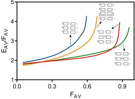
3.13 Optimal (Pareto) curves of eluent consumption (Eav/Fav) versus

average feed flow rate (Fav), for solution of the separation

prob-lem defined in Table 3.1 with the batch and SSR configurations of Figs. 3.9 and 3.11 . . . 39

3.14 Schematic of the operating cycle (2τ) for the two-column, open-loop process with continuous elution . . . 40

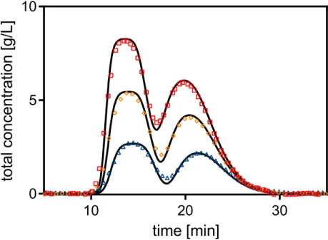
3.15 Solute concentration profile at the outlet of the system, for the two-column, open-loop operation with continuous elution defined in Table 3.3 . . . 41

3.16 Steady periodic solution of the axial composition profile for the first switching interval for the two-column, open-loop operation with continuous elution defined in Table 3.3 . . . 42

3.17 Schematic of the operating cycle (2τ) for the two-column, open-loop process with discontinuous elution . . . 43

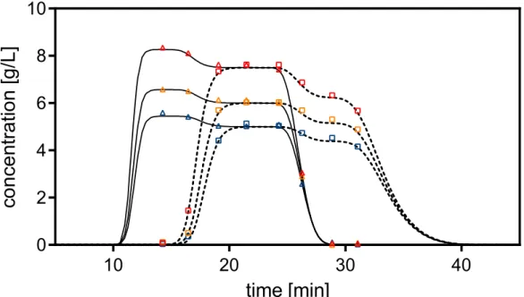
3.18 Solute concentration profile at the outlet of the system, for the two-column, open-loop operation with continuous elution defined in Table 3.4 . . . 44

(17)

3.20 Optimal (Pareto) curves of eluent consumption (Eav/Fav) versus

average feed flow rate(Fav), for solution of the separation problem

defined in Table 3.1 with the configurations of Figs. 3.9, 3.11, 3.14 and 3.17 . . . 46

4.1 Schematic of a four-zone SMB . . . 54

4.2 Schematic of basic idea behind the relay SMB . . . 57

4.3 Schematic of the R-SMB’s operating cycle forα_≤(3 +√5)/2 . . . 59 4.4 Equilibrium solution for complete separation of a linear adsorption

system, for which α < (3 +√5)/2, by the R-SMB−

process under optimal operating conditions (E′

/F = 1 . . . 62 4.5 Schematic of the operating cycle for the R-SMB+_{process, which is}

applicable whenα _≥(3 +√5)/2 . . . 64 4.6 Equilibrium solution for complete separation of a linear adsorption

system, for which α > (3 +√5)/2, by the R-SMB+ _{process under} optimal operating conditions (E′

/F = 1 . . . 66 4.7 Desorbent consumption (E′

/F) and specific productivity (F/V′

1) as a function of P´eclet number per column (Pe) for complete separation (PR = PX = 0.99) of a linear adsorption system (α = 1.4) with

different four-column configurations . . . 74

4.9 Desorbent consumption (E′

/F) and specific productivity (F/V′

1) as a function of P´eclet number per column (Pe) for complete separation (PR = PX = 0.99) of a linear adsorption system (α = 3.0) with

different four-column configurations . . . 76

4.10 Specific productivity (F/V′

1) and desorbent consumption (E

′

/F) as a function of selectivity (α) for complete separation (PR = PX =

0.99) of a linear adsorption system at a P´eclet number per column Pe = 200with different four-column configurations . . . 77

4.11 Specific productivity (F/V′

1) and desorbent consumption (E

′

/F) as a function of selectivity (α) for complete separation (PR = PX =

(18)

5.1 Schematic of the four-column SMB unit used in the experimental runs. 90

5.2 Schematic of the R-SMB process for the two selectivity regions . . . 92

5.3 Solute concentration profiles at the outlet of column 1 for the chro-matographic parameters given in Table 5.2 for the R-SMB process withα < αC . . . 92

5.4 Solute concentration profiles at the outlet of column 1 for the chro-matographic parameters given in Table 5.2 for the R-SMB process withα > αC . . . 93

5.5 Shematic of the open-loop smb with recycle process . . . 93

5.6 Pareto Plots forα < αC andα > αC . . . 94

6.2 Flow diagrams of the feed and production steps for the case when they occur at the beginning of the third switching interval and when the product withdrawal takes longer than the injection of feed. . . 103

6.3 Schematic flowsheet of the GSSRpilot unit. . . 104

6.4 Cycle sequence chosen in the moving solvent-gradient implementation.109

6.5 Accumulated mass from the product (top) and waste (bottom) out-lets as function of elapsed time (t/τ) for one complete cycle of the GSSR process, with operating parameters defined in Table 6.1 . . . 110

6.6 Temporal profile of blue dextran concentration at the outlet of col-umn 3 for 5 cycles of a GSSRprocess . . . 111

7.1 Peak deconvolution for an analytical chromatogram of the crude peptide mixture . . . 119

7.2 Henry constants, Ki = (1−ǫb)Hi, for the key components of the

peptide mixture, as a function of EtOH concentration . . . 121

7.3 Henry constants,Ki = (1−ǫb)Hi, for the target peptide (i= 2) and

its two closest impurities (i = 2and i = 3), as a function of EtOH concentration . . . 122

(19)

7.5 Effect of the switching interval,τ, on the elution time of the main product peak at the outlet of the column where the product fraction is collected. . . 132

7.6 Temporal profile of the UV signal measured at the outlet of column 3 for the 30-cycleGSSRexperiment. . . 133

7.7 Temporal profile of the UV signal measured at the outlet of column 3 for the last four cycles of the 30-cycleGSSRexperiment. . . 134

7.8 HPLC analysis of the product fraction collected during the last cycle of the 30-cycleGSSRexperiment of Fig. 7.6 . . . 135

7.9 Simulated curve of optimal product recovery (recp) versus purity

(pur_p) for single-column batch chromatography (SCBC) subject to the same amount of stationary phase and amount of feed injected per cycle as in the 30-cycleGSSR experiment. . . 137

8.1 Standard batch downstream train for virus purification. . . 143

8.2 Pulse experiments in isolated and connected columns. . . 151

8.3 Set of suitable flow-path configurations for the design of a two-column, open-loop SEC process without partial splitting of exit streams. . . 152

8.4 Schematic representation of operating cycle for the two-column, semi-continuous open loop process. . . 154

8.5 Steady state profile at the inlet/outlet of the first switching interval. 155

8.6 Modeled profile of the two-column during the semi-continuous cycle.156

8.7 Experimental chromatogram representing the automatic column cycling during the continuous SEC purification. . . 156

(20)

List of Tables

3.1 Column characterization and adsorption parameters for the nonlin-ear separation of Tr¨oger’s base enantiomers on Chiralpak AD and ethanol at 25◦_{C . . . .} ₃₄

3.2 Optimal operating cycle for the solution of the separation problem defined in Table 3.1 with a batch configuration (Fig. 3.9) . . . 36

3.3 Optimal operating cycle for the solution of the separation problem defined in Table 3.1 with a two-column, open-loop configuration with continuous elution (Fig. 3.14) . . . 40

3.4 Optimal operating cycle for the solution of the separation problem defined in Table 3.1 with a two-column, open-loop configuration with discontinuous elution (Fig. 3.17) . . . 43

4.1 Summary of the design equations, derived from the equilibrium theory, for the optimum operation of the two R-SMB cycles that give complete separation under linear adsorption conditions . . . 68

4.2 Linear adsorption column model. . . 68

5.1 Column characterization and adsorption parameters for the linear separation of uridine/guanosine and uridine/adenosine on Source 30 RPC (reversed phase) and 5% (v/v) ethanol in water at 30◦

C . . 91

5.2 Optimal cycle parameters for the R-SMB processes . . . 91

5.3 Purities of the experimental runs for the R-SMB processes . . . 91

6.1 Operating parameters of theGSSRcycle . . . 109

7.1 Values of ǫ+Ki for the key components of the peptide mixture, as a

function EtOH concentration . . . 120

(21)

8.1 Characterization of the two columns packed with Sepharose 4FF. . 148

8.2 Model parameters derived from analysis of pulse experiments per-formed on the two columns placed in series. . . 152

(22)

(23)

Resumo

A recente redução de escala da tecnologia de Leito Móvel Simulado (LMS) possibili-tou o aparecimento de novas aplicações, como a purificação de produtos de qu´ımica fina, ácidos orgânicos, produtos de ´ındole farmacêutica, anticorpos monoclonais e prote´ınas recombinantes. O nosso grupo desenvolveu recentemente uma nova classe de processos LMS semi-cont´ınuos que utilizam duas colunas cromatográficas em anel aberto. Estes processos exploram os benef´ıcios do processo LMS mas, utilizando uma configuração de nodos flex´ıvel, uma operação robusta das bombas e modulação c´ıclica dos caudais. A grande vantagem do processo sugerido é a sua simplicidade de operação pois, independentemente do número de colunas, são apenas necessárias duas bombas – uma para a adição de alimentação e outra para a adição de dessorvente – bem como válvulas simples com uma operação on-off, por forma a controlar os caudais de fluidos retirados do sistema. A performance do nosso processo foi testada com sucesso numa separação enantiomérica não linear, usando duas estratégias de eluição.

(24)

Em muitos dos problemas de purificação de produtos biológicos, o composto desejado encontra-se numa posição intermédia entre dois grupos de impurezas - menos ou mais adsorvidas. Um corte central é, então, uma alternativa viável para a recuperação do produto de interesse. O processo de reciclo em estado estacionário com gradientes (GSSR) é composto com um sistema multi-coluna em anel aberto com um gradiente de solventes e uma operação em estado estacionário c´ıclico. É especialmente indicado para separações ternárias, visto que possibilita a existência de três fracções ou produtos, sendo o produto de interesse contido na fracção intermédia. Uma descrição detalhada do processo GSSR é fornecida, realçando a sua versatilidade, flexibilidade e simplicidade de operação. A validação experimental numa unidade piloto é também fornecida, usando para este fim a separação de uma mistura de prote´ınas em fase reversa como referência e caso de estudo.

(25)

Abstract

The recent scale-down of the Simulated Moving Bed (SMB) technology led to new applications, including the purification of fine chemicals, organic acids, pharmaceu-tics, monoclonal antibodies, and recombinant proteins. We developed a novel class of semi-continuous, two-column, open-loop SMB systems. These processes exploit the benefits of the SMB but with a flexible node design, robust pump configuration, and cyclic flow-rate modulation. The major advantage of our design is the simplic-ity of its physical realization: regardless of the number of columns, it uses only two pumps — one to supply feed and another to supply desorbent — and simple two-way valves to control the flow rates of liquid withdrawn from the system. The performance of our process was successfully tested on a nonlinear enantiomeric separation, using two types of elution strategies.

The operating principle of our two-column SMB systems discards the splitting of the flow into two or more streams at an active outlet: the product, waste, or recycled fractions are always obtained by completely directing the effluent over a certain period of the cycle to the appropriate destination. This strategy of handling the product outlets was also explored in the Relay SMB. In this process, the analogy with the standard SMB in terms of displaced volumes of fluid per switch interval is maintained, whilst avoiding the use of flow controllers or an extra pumps. In this process the flow through a zone (or column) is always in one of the three states: (i) frozen, (ii) completely directed to the next zone (or column), or (iii) entirely diverted to a product line. For this class of processes we derive a SMB analog — the R-SMB process and demonstrate, under the framework of the equilibrium theory, that this process has the same separation region as the classical SMB for linear adsorption systems. In addition, the results from the equilibrium theory show that the R-SMB process consists of two distinct cycles that differ only in their intermediate sub-step depending on the selectivity of a given separation.

(26)

operation. It is particularly suited for ternary separations: it provides three main fractions or products, with a target product contained in the intermediate fraction. A comprehensive description of the GSSR process is given, highlighting the versatility, flexibility, and ease of operation of the process. The experimental validation in a pilot unit is provided, using the purification of a crude peptide mixture by reversed phase as a benchmark and case study.

(27)

1

Introduction

1.1 Relevance and Motivation

Chromatography is one of the simplest, yet effective, separation methods, able to separate any soluble or volatile component if the right column configuration, operating conditions, mobile phase, and stationary phase are employed. Batch chromatography, because of its ease of operation and low capital investment, is a well-established process used in many large-scale industries, like sugar processing, and to some extent in the hydrocarbon industry; also chromatography proven to be very useful, as both an analytical and preparative or process-scale purification, in small-scale applications such as the pharmaceutical, biotechnology, fine chemistry, and food processing industries. Although batch chromatography can be very flexible, allowing the recovery of several fractions from a feed mixture in a single operation, it suffers from the drawbacks of batch operation, the products are recovered at a high dilution rate, the stationary phase is not efficiently used, and the purity of the recovered fractions is extremely dependent on the selectivity of the chromatographic system.

(28)

chromatogra-1.1. Relevance and Motivation

phy (not to be confused with liquid-liquid countercurrent chromatography). In a binary separation, the moving bed achieves of high purity, even if the resolution of the system is not excellent, because only the purity at the two tails of the concentra-tion profiles, where the withdrawal ports are located, is of interest. This is contrary to batch chromatography where the purity of the products is dependent of the system resolution. It is also clear that the loading of the stationary phase is higher in a moving bed than in a fixed bed system, which leads to a higher productivity per unit mass of stationary phase. However, the advantages of theTMBprocess are rapidly overcome by the difficulty of its physical realization; therefore, in practice the continuous movement of the stationary phase is simulated in a discrete way by replacing the moving bed by a circular train of fixed beds packed with the stationary phase and periodically moving the inlet and outlet ports in the same direction as the fluid flow—this is the Simulated Moving Bed (SMB) process.

The first large-scale commercial application of continuous simulated countercurrent adsorption was developed by UOP (Universal Oil Products, Des Plaines, Illinois, USA) in the early 1960s, under the generalized name of Sorbex.

In the last decades, the scaling-down of the SMB technology led to a new set of applications, especially in the purification of fine chemicals, organo acids, phar-maceutics, monoclonal antibodies, or recombinant proteins. A new trend in SMB processes emerged from the demands of these new type of applications. Smaller and more versatile configurations are preferred, no longer making use of the initial process configuration where several columns with large dimensions were employed. The moving trend is supported by an increase in complexity, which in most cases requires highly versatile equipment and advanced optimization tools.

Although the SMB process increases throughput, purity, and yield relative to batch chromatography, the batch process still presents the obvious advantages of being easy to operate, requiring a low capital investment, and being easily prone to the application of solvent gradients or center-cut separations.

(29)

1.2. Objectives and Outline

1.2 Objectives and Outline

This thesis is organized into nine chapters. The present chapter describes the relevance and motivation of the work as well as the structure of the thesis.

Chapter 2 introduces the principles of TMB and SMB chromatography. Moreover, a brief review of the state of the art on the SMB processes and applications is included. This chapter finalizes with an introduction to chromatographic separation techniques used for the separation of biological products.

Chapter 3 presents a proof of concept of the application of a streamlined, two-column SMB system, developed by our group, to a nonlinear chiral separation problem. In this chapter we also present two different elution strategies that can be implemented in the two-column system. These strategies are analyzed numerically and compared to the reference cases of batch chromatography and steady-state recycling. This chapter is based on the submitted paper to Journal of Chromatography A:

• R.J.S. Silva, R.C.R. Rodrigues, J.P.B Mota, Two-column streamlined simulated moving bed applied to a nonlinear chiral separation.

Chapter 4 deals with the concept and design criteria for a new class of multicolumn chromatographic processes that change the classical way of handling the product outlets of simulated moving-bed (SMB) chromatography to avoid the use of flow controllers or an extra pump. Despite the simplified manipulation of the zone flow rates, the R-SMB process maintains the analogy with the SMB in terms of displaced volumes of fluid per switch interval. This chapter is based on work published in

• Ricardo J.S. Silva, Rui C.R. Rodrigues, Jos´e P.B. Mota, Relay simulated moving bed chromatography: Concept and design criteria, Journal of Chromatogra-phy A, 1260 (2012),132-142.

Chapter 5 presents the experimental validation of the Relay simulated moving bed concept, presented in the previous chapter. This chapter is an extension of the previous work done in this field

(30)

1.2. Objectives and Outline

• Ricardo J.S. Silva, Rui C.R. Rodrigues, Hector Osuna-Sanchez, Michel Bailly, Eric Val´ery, Jos´e P.B. Mota, A new multicolumn, open-loop process for center-cut separation by solvent-gradient chromatography, Journal of Chromatogra-phy A, 1217 (2010), 8257-8269.

Chapter 7 deals with the model-based analysis of the process and the optimal cycle design. We also report on the experimental validation of this process. The work described in the previous chapter and in the present one is summarized and some conclusions are drawn.

Chapter 8 describes the application of the two column simulated moving bed system, using size exclusion chromatography, in the purification of adenovirus. This chapter is based on the paper submited to Journal of Chromatography A:

• Piergiuseppe Nestola, Ricardo J.S. Silva, Jos´e P.B. Mota, Adenovirus purifica-tion by two-column, size-exclusion, simulated countercurrent chromatogra-phy.

(31)

2

Simulated Moving Bed technology: a

brief review

2.1 Introduction

The Simulated Moving Bed (SMB) is a multicolumn, continuous, countercurrent adsorption separation process that, generally speaking, increases throughput, purity, and yield. The first large-scale commercial application of continuous simulated counter-current adsorption was developed by UOP (Universal Oil Products) in the early 1960s, since then, the SMB technology has been widely used in the petrochemical (xylene isomer separation) and food industries (glucose-fructose separation) on a multi-ton scale. In the last two decades, with the advent of stable bulk stationary phases for chromatographic enantioseparation, the SMB principle has been successfully transferred to the pharmaceutical industry.

(32)

2.2. Principle of SMB Technology: the concept of True Moving Bed

modeling and simulation for reliable process design and optimization.

2.2 Principle of SMB Technology: the concept of True

Moving Bed

The operation of a SMB unit can be best understood by means of the ideal concept of the TMB, which involves the actual circulation of the solid at a constant flow rate in opposite direction to the fluid phase. Furthermore, liquid and adsorbent streams are continuously recycled as shown in figure 2.1. The feed is continuously injected into the middle of the system and two product lines are collected: the extract, rich in the more retained components, and preferentially carried with the solid phase, and the raffinate, rich in the less retained components that move with the liquid phase. Also, pure solvent is continuously injected at the beginning of section I and admixed with the liquid recycled from the downstream end of section IV.

Feed Raffinate

Extract Desorbent

Section I Section II Section III Section IV

B A

concentration

axial coordinate Solid phase Liquid phase

Figure 2.1: Schematic of a four-section TMB. The separation A and B is carried out in sections II and III. The collection of products A and B is performed in the extract and raffinate streams, respectively.

(33)

2.2. Principle of SMB Technology: the concept of True Moving Bed

and carried by the mobile phase in the direction of the raffinate port. In section I the solid is regenerated by desorption of the strongly adsorbed component with fresh eluent stream. Finally, in section IV the liquid is regenerated by adsorption of the less retained component that was not collected in the raffinate. With this arrangement it is possible to recycle back both the solid and liquid phase to sections IV and I, respectively. With a proper choice of the internal flow rates and solid phase velocity, the feed mixture can be completely separated into two pure products, even if the resolution of the system is not excellent because only the purity at the tails of the concentration profiles, where the withdrawal ports are located, is of interest. This is contrary to batch chromatography, where high resolution is vital in order to achieve high purity. It is also evident that a larger portion of the stationary phase is loaded in the moving-bed system than in a fixed-bed system. This will ultimately lead to a higher productivity per unit mass of stationary phase.

However, the movement of the adsorbent particles, which are in most cases within the micrometer range, is technically unfeasible as a result of particle attrition and backmixing. Therefore, in practice the movement of the solid phase is simulated by using fixed beds of adsorbent (chromatographic columns) and periodically moving the inlet and outlet ports in the same direction as the fluid flow. The simulated countercurrent behavior of the process becomes obvious when the relative move-ment of the packed beds with respect to the inlet and outlet streams is followed over several switching intervals (a switching interval is the time interval between consecutive switches of the positions of the inlet and outlet ports). After a number of switching intervals equal to the number of columns in the system, one cycle is completed and the initial positions of all external streams are reestablished.

Due to the continuous nature of countercurrent operation, after the initial transient start-up a TMB unit attains a steady state. On the contrary, the steady regime attained by the discrete movement of the solid in a SMB unit is periodic, that is, it exhibits the same time-dependent behavior over every switching interval.

(34)

2.3. SMB process

relationships:

Vj =NjV (2.1)

V τ =

QS

1₋ǫ (2.2)

QSM B_j =QT M B_j + QS

1₋ǫ (2.3)

HereV is the volume of a SMB column whereasVj is volume of thejthsection of

the TMB unit;Nj is the number of subsections in thejthsection of the SMB unit,τ

is the length of the switching interval of the SMB unit, ǫis the void fraction of the adsorbent bed, QS, is the volumetric solid flow rate in the TMB unit, andQSM Bj

andQT M B

j are, respectively, the volumetric fluid flow rates in the equivalent SMB

and TMB units.

2.3 SMB process

Classical SMB systems are characterized by the synchronous and downstream shifting by one column of all inlet and outlet lines after a defined switching interval

τ. As mentioned above, in a classical SMB it is possible do distinguish four different sections defined by different liquid flow rates (figure 2.2). The number of columns may be evenly distributed or not over the four sections; however, by definition each section has an integer number of columns,NI/NII/NIII/NIV, and the sum of the

number of columns over the four sections is equal to the total number of columns. Fig. 2.2 shows an example of a SMB system with a1/2/2/1column configuration.

2.4 SMB operation with variable parameters

(35)

2.4. SMB operation with variable parameters

E X F R

t

E X F R

t+τ

Figure 2.2: Schematic diagram of a four-section SMB unit for two consecutive switching intervals, where the upper diagram depicts the instantt, and the bottom diagram depicts the instantt+τ where the input and withdrawl ports are moved one column ahead. The position of eluent (E), feed (F), extract (X), and raffinate (R) ports are identified by arrows.

considered.

2.4.1 Varicol

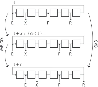
The Varicol process [1, 2] generically consists of performing a predetermined sequence of asynchronous port switchings over every switching interval, resulting in a time-periodic modulation of the zone lengths. When the process dynamics is averaged over a complete cycle the Varicol scheme is equivalent to a non-integer allocation of the number of columns per section. The possibilities for asynchronous port switching are endless; for example, in principle it is possible that a port may shift more than once during the switching interval, either forward or even backwards. As a result, Varicol schemes can have an infinite number of column configurations though only a small subset of them will give rise to high-performance processes.

(36)

E X F R

t

E X F R

t +τ

t +ατ (α< 1 )

E X F R

SMB

V

ARICOL

Figure 2.3: Simplified scheme of the Varicol process. The position of eluent (E), feed (F), extract (X), and raffinate (R) ports are identified by arrows.

2.4.2 PowerFeed

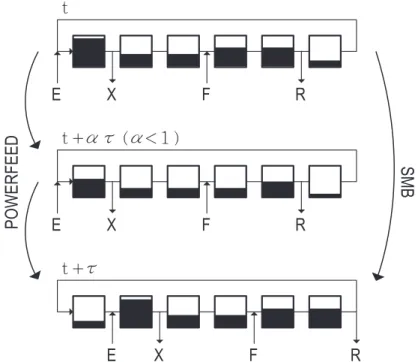
This concept was originally introduced by Kearny and Hieb [3], and studied in more detail by other authors [4–6]. Like the conventional SMB process, the switching of the external ports are kept constant, in contrast to the Varicol process. The additional performance improvement is created by the modulation of some or all flow rates during each switching interval. Consequently, the internal flow rates also change within a switching period. Fig. 2.4 shows an example of the Powerfeed process, where the shaded areas are proportional to the flow rate in the corresponding section.

2.4.3 ModiCon

(37)

SMB

POWERFEED

E X F R

t

E X F R

t +τ

t +ατ (α< 1 )

E X F R

Figure 2.4: Simplified scheme of the PowerFeed process. The position of eluent (E), feed (F), extract (X), and raffinate (R) ports are identified by arrows. The height of each shaded area is proportional to the flow-rate through the corresponding section. The standard SMB scheme keeps the topmost configuration constant over the whole switching intervalτ; all ports are then switched forward by one column in the direction of fluid flow. In PowerFeed operation, which is illustrated by the intermediate step, the flow-rates are varied over a fraction of the switching interval but the ports are only moved forward by one column at the end of the step like in the standard SMB process.

2.4.4 Improved-SMB or Intermittent-SMB

(38)

t t +τ time

F

e

d

C

o

n

c

e

n

tr

a

ti

o

n

t + 2τ

Figure 2.5: Temporal profiles of the Feed concentration in the standard SMB (in red) and Modicon (in blue) over two consecutive switching intervals. Both processes are character-ized for a fixed section configuration over the switching intervals. In the exemplified case a period of the switching interval is characterized by a pure eluent feed (cF = 0), followed by a step wave where cF is two times the feed concentration of the equivalent SMB process.

2.4.5 Partial-Feed, Partial-Withdrawal/Discard and Outlet-Swing

Stream SMB

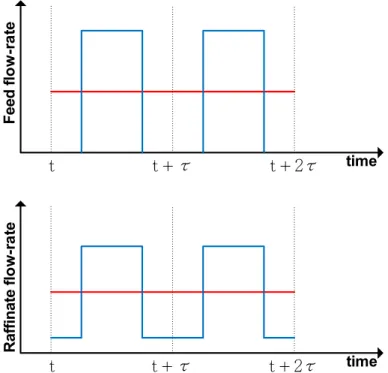
In the classical SMB process the composition and flow rate of the feed is constant over the whole switching interval. The approach in the Partial-Feed [12] process introduces two more degrees of freedom, the feed duration and feed time. Fig. 2.7 depicts the flow-rate of the feed and raffinate ports in a Partial-Feed operation. As one can easily understand, in order to fulfill the mass balance constraints the raffinate flow rate changes according to the variation of the feed flow. In the case of the Partial-Feed operation the duration of the feed is shorter, but the introduced flow rate is higher. By this procedure the total amount of feed is kept constant, while productivity and eluent consumption may increase.

The concept of partial withdrawal [13], which is based on the variation of the raffinate flow rate in a three-zone SMB, can be used to withdraw the more con-centrated part of the profile or to leave inside the system the most diluted part, respectively. As a consequence, the eluent consumption can be decreased for a given purity requirement. An analogous operation is the so-called partial-discard. In this case, although the recovery of the two product outlets is complete, only a part of the outlet is kept in order to improve the overall purity and the remaining is discarded [14] or recirculated back to the feed [15, 16].

(39)

t + ατ (α< 1 )

E X F R

t

E X F R

t +τ

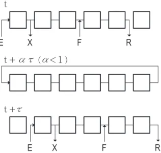
Figure 2.6: Port configuration of an I-SMB scheme for two consecutive switching intervals. In this process, the inlet and outlet ports are only active in a certain period of the switching interval, this is followed by a step of internal recycling at a discrete flow-rate.

contract the product fronts near the withdrawal points, by manipulating the outlet flow rates, thus allowing the variation of flow rates in sections I and IV while keeping the flow rates in sections II and III constant by modulating the eluent flow rate.

2.4.6 Other examples of non-standard SMB operation

The 3-zone SMB scheme is probably one of the simplest schemes that deviates from the classical 4-zone SMB [18]. This configuration relies on the removal of zone IV, letting all fluid coming from zone III to be collected as raffinate, which prevents any contamination of the extract coming from the recirculation line.

More recently, Jin and Wankat [19] theoretically derived a 2-zone SMB for binary separation in which they incorporate a storage tank to temporarily hold the solvent for later use. One-column processes that reproduce the cyclic behavior of the multicolumn SMB chromatography by means of a recycle lag have also been proposed [20, 21]. This setup exploits the cyclic behavior of the SMB where all columns are subjected to the same inlet/outlet concentration waveform everyN τ

time units.

(40)

time

Feed f

lo

w

-r

a

te

t t + τ t + 2τ

time

Raffinate f

lo

w

-r

a

te

t t + τ t + 2τ

Figure 2.7: Feed and Raffinate flow-rates of a Partial-Feed operation for two consecutive switching intervals.

of more than two components and the goal is, in many cases, to isolate one component that is intermediately retained in the columns. The first logical step to achieve a “center-cut” separation is to implement a cascade of two [22, 23] or even more [24] SMB units, making a series of partitions to isolate the desired product. Although this is a very straightforward solution, it has an economical drawback since the need of several SMB units implies the use of much more equipment.

2.4.7 Gradient elution in SMB processes

One characteristic of the SMB processes described so far is that they are all operated under isocratic, isothermal conditions with nearly-incompressible liquid phases where the thermodynamic effect of pressure changes is negligible. During the selection of both stationary and fluid phase, one of the main goals is to find a sepa-ration method where the first component is fairly well adsorbed on the stationary phase while the second one can still be easily eluted under those conditions. The elution strength can be controlled by changing the composition of the solvent or desorbent. A solvent gradient can improve the SMB separation if the selectivity of the components is small or if the separation under isocratic conditions is impossible.

(41)

a (semi-)continuous, countercurrent, multicolumn chromatography process capable of performing three-fraction separations by changing the solvent composition along the system [25, 26]. This process can be used either for the purification of a single species from a multicomponent mixture or to separate a three-component mixture in a single operation. As shown in the scheme of Figure 2.8, the continuous 6-column MCSGP process consists of a group of 3 columns that are interconnected and another 3 columns that operate in batch mode; the interconnected columns implement the separation gradient like in batch chromatography; the disconnected columns perform the loading, the elution of the target product, and the elution of strongly adsorbed species plus washing, cleaning-in-place, and re-equilibration. In between the interconnected columns additional inlet streams are used to adjust the required solvent composition in order to reproduce the desired solvent gradient. This process can be operated discontinuously with only three columns [27].

I W

F

S P

Figure 2.8: A schematic diagram of the MultiColumn Solvent Gradient Process (MCSGP). It is a fully continuous system comprising 6 chromatographic columns using solvent gradient for a three-fraction separation/purifications. Like in the SMB process, the system moves one column ahead every switching interval. S are the strongly adsorbing impurities, P is the target product, W are the weakly adsorbing impurities, I the inerts or very weakly adsorbing impurities and F the feed mixture.

(42)

References

[1] Philippe Adam, Roger Narc Nicoud, Michel Bailly, and Olivier Ludemann-Hombourger. Process and device for separation with variable-length, Octo-ber 24 2000. US Patent 6,136,198.

[2] O Ludemann-Hombourger, RM Nicoud, and M Bailly. The varicol process: a new multicolumn continuous chromatographic process. Separation Science and Technology, 35(12):1829–1862, 2000.

[3] Michael M Kearney and Kathleen L Hieb. Time variable simulated moving bed process, April 7 1992. US Patent 5,102,553.

[4] E Kloppenburg and ED Gilles. A new concept for operating simulated moving-bed processes. Chemical engineering & technology, 22(10):813–817, 1999.

[5] Ziyang Zhang, Marco Mazzotti, and Massimo Morbidelli. Powerfeed operation of simulated moving bed units: changing flow-rates during the switching interval. Journal of Chromatography A, 1006(1):87–99, 2003.

[6] Ziyang Zhang, Massimo Morbidelli, and Marco Mazzotti. Experimental assess-ment of powerfeed chromatography. AIChE journal, 50(3):625–632, 2004.

[7] Henning Schramm, Malte Kaspereit, Achim Kienle, and Andreas Seidel-Morgenstern. Improving simulated moving bed processes by cyclic mod-ulation of the feed concentration. Chemical engineering & technology, 25(12): 1151–1155, 2002.

[8] H Schramm, A Kienle, M Kaspereit, and A Seidel-Morgenstern. Improved operation of simulated moving bed processes through cyclic modulation of feed flow and feed concentration. Chemical engineering science, 58(23): 5217–5227, 2003.

(43)

References

[10] Kenzaburo Yoritomi, Teruo Kezuka, and Mitsumasa Moriya. Method for the chromatographic separation of soluble components in feed solution, May 12 1981. US Patent 4,267,054.

[11] Florence Lutin, Mathieu Bailly, and Daniel Bar. Process improvements with innovative technologies in the starch and sugar industries. Desalination, 148 (1):121–124, 2002.

[12] Yifei Zang and Phillip C Wankat. Smb operation strategy-partial feed. Indus-trial & engineering chemistry research, 41(10):2504–2511, 2002.

[13] Yifei Zang and Phillip C Wankat. Three-zone simulated moving bed with partial feed and selective withdrawal. Industrial & engineering chemistry research, 41(21):5283–5289, 2002.

[14] Youn-Sang Bae and Chang-Ha Lee. Partial-discard strategy for obtaining high purity products using simulated moving bed chromatography. Journal of Chromatography A, 1122(1):161–173, 2006.

[15] Andreas Seidel-Morgenstern, Lars Christian Keßler, and Malte Kaspereit. New developments in simulated moving bed chromatography.Chemical engineering & technology, 31(6):826–837, 2008.

[16] Lars Christian and Seidel-Morgenstern. Method and device for chromato-graphic separation of components with partial recovery of mixed fractions, August 25 2010. EP Patent 1,982,752.

[17] Pedro S´a Gomes and Al´ırio E Rodrigues. Outlet streams swing (oss) and mul-tifeed operation of simulated moving beds. Separation Science and Technology, 42(2):223–252, 2007.

[18] Douglas M Ruthven and CB Ching. Counter-current and simulated counter-current adsorption separation processes. Chemical Engineering Science, 44(5): 1011–1038, 1989.

[19] Weihua Jin and Phillip C Wankat. Two-zone smb process for binary separation.

Industrial & engineering chemistry research, 44(5):1565–1575, 2005.

(44)

References

[21] Nadia Abunasser and Phillip C Wankat. One-column chromatograph with recy-cle analogous to simulated moving bed adsorbers: Analysis and applications.

[22] Phillip C Wankat. Simulated moving bed cascades for ternary separations.

[23] Jeung Kun Kim, Yifei Zang, and Phillip C Wankat. Single-cascade simulated moving bed systems for the separation of ternary mixtures. Industrial & engineering chemistry research, 42(20):4849–4860, 2003.

[24] Jeung Kun Kim and Phillip C Wankat. Designs of simulated-moving-bed cas-cades for quaternary separations. Industrial & engineering chemistry research, 43(4):1071–1080, 2004.

[25] Lars Aumann and Massimo Morbidelli. Method and device for chromato-graphic purification, November 2 2006. EP Patent 1,716,900.

[26] Guido Str¨ohlein, Lars Aumann, Marco Mazzotti, and Massimo Morbidelli. A continuous, counter-current multi-column chromatographic process incorpo-rating modifier gradients for ternary separations. Journal of Chromatography A, 1126(1):338–346, 2006.

(45)

3

Two-column open-loop system for

nonlinear chiral separation

3.1 Introduction

The simulated moving bed (SMB) is a continuous adsorption separation process with numerous applications, many of which are difficult or even impossible to handle using other separation techniques. The SMB process was originally devised as a practical implementation of the true moving bed (TMB) process, where the adsorbent and the fluid phase move counter-currently [1–3].

A binary feed (A/B) may be separated by SMB into two products: an extract product containing mainly solute A (the more strongly adsorbed species, or group of species with similarly strong adsorption properties) and a raffinate containing mainly solute B (the less strongly adsorbed species or group of species). SMB chromatography increases throughput, purity, and yield relative to batch chromatography [4–7].

(46)

3.1. Introduction

Concepts such as asynchronous port switching [8–10], cyclic modulation of feed concentration [11, 12], time-variable manipulation of the flow rates [13–17], and solvent-gradient operation [18–21], have been thoroughly analyzed. The extra degrees of freedom available with these schemes improve the separation efficiency, thus allowing for the use of units with less columns than traditionally used. The advantages are apparent: less stationary phase is used, the set-up is more economic, and the overall pressure drop can be reduced. Furthermore, switching from one mixture to another is easier and takes less time than with more columns.

The classical implementation of the SMB process comprises four zones, with an integer number of columns per zone. Alternatives to this standard operation scheme, with less zones, have also been studied. For example, the three-zone SMB configuration [3, 22, 23] takes the four-zone, open-loop SMB and removes zone IV. If the amount of adsorbent allocated to each zone is properly optimized by means of asynchronous port switching, then a three-zone asynchronous SMB can perform better than a standard (i.e., synchronous) four-zone SMB [24–26]. The advantages and drawbacks of the three-zone SMB have been discussed by Chin and Wang [27]. Another example of a system that uses less zones was proposed by Lee [28], where a two-zone SMB with continuous feeding and partial withdrawal was used for glucose-fructose separation; this process appears to be more suitable for enriching products than for high-purity separations [27]. Another example of a two-zone SMB scheme uses intermittent feeding and withdrawal to achieve ternary separations [29].

Jin and Wankat [30, 31] developed more recently other examples of two-zone SMBs for binary separation, which incorporate a storage tank to temporarily hold desorbent for later use. Their results show that good separation can be achieved but with more desorbent than required by a four-zone SMB. However, partial feed was shown to improve the product purities and recoveries considerably. The system was subsequently extended to ternary separations [32], and a different two-zone SMB system, which does not use a storage tank, was developed for center-cut separation from ternary mixtures [33]. Other processes particulary suitable for ternary separations are the MCSGP [34] and the GSSR [21] processes; these systems incorporate the principle of counter-current operation and the possibility of using solvent gradients. One-column processes that reproduce the cyclic behavior of multicolumn SMB chromatography, by means of a recycle lag, have also been proposed [35–37].

(47)

3.1. Introduction

flexible node design, robust pump configuration, and cyclic flow-rate modulation to exploit the benefits of both batch and simulated counter-current modes [38]. We emphasize the use of two columns rather than two zones, because with three or more columns it is always possible to implement a better SMB scheme which uses more zones with roughly the same ancillary equipment. In fact, running a two-zone configuration with three columns can be detrimental to the separation because the zone lengths become highly asymmetrical [39].

One advantage of our streamlined design is the simplicity of its physical realization: the simplest configuration, with no recirculation step, requires only two pumps to supply feed and desorbent into the system, while the flow rates of liquid withdrawn from the system are controlled by material balance using simple two-way valves. This type of operation implicitly discards the possibility of splitting into two or more streams the flow exiting one column; in this sense, the product, waste, or recycling fractions are always obtained by completely directing the effluent over a certain period of the cycle to the appropriate destination. The different port configurations that can be implemented with our simplest streamlined design are depicted in Fig. 3.1. In the present work a series of two-column open-loop processes

(a)

(b) (c)

(d)

(g) (f )

(e)

Figure 3.1: Possible port configuration between two consecutive columns, or group of columns: (a) complete direction of flow to the next column; (b) downstream frozen bed; (c) upstream frozen bed; (d) flow addition to circulating stream; (e) complete withdrawal and flow injection at the same node; (f) partial withdrawal, and (g) partial withdrawal and flow addition at the same node. Configurations (f) and (g) are not considered, as they imply partial withdrawal of the exit stream from a column.

(48)

3.2. Experimental Setup

This chapter is organized as follows. We start by describing the experimental setup where the proofs of concept were realized, discuss the procedure for optimal cycle design, and then the numerical approach used to solve the resulting nonlinear programming problem. We then report on the experimental verification of the performances of the two-column processes, using the nonlinear separation of Tr¨oger’s base in Chiralpak AD as a convenient model separation problem. The experiments not only support the discussion of the results but also validate the modeling tools employed in a comparison study of the processes assessed. Finally, the work is summarized before drawing final conclusions.

3.2 Experimental Setup

Fig. 3.2 shows a schematic of the node configuration employed in our prototype apparatus. As stated above, the flow rate of liquid that is withdrawn at each node is controlled by material balance. The versatility of the valves used, allows the easy implementation of the port configurations (a)-(e) depicted in Fig. 3.1. Two-way

Column 1

Column 2

UV cell

X

R F

E

F R

X

UV cell

FC

Figure 3.2: Schematic diagram of semi-continuous, two-column, open-loop chromatograph for chiral separation.

(49)

3.3. Model based cycle design

to the other column. This valve is normally open and is only closed when the effluent from the upstream column is totally withdrawn as product or the fluid in the column needs to be temporarily frozen. Overall, each set-up employs 10 two-way valves to control the port switching. The two-two-way valves are model SFVO from Valco International (Schenkon, Switzerland) with pneumatic actuation. Each valve is automated by means of a single computer-controlled three-way solenoid: application of 50 psi opens the valve; venting the air allows the spring to return the valve to the closed position.

The inlets of the chromatographic unit are represented in detail in Fig.3.3. This valve scheme allows the recycling of the desorbent or feed stream back to the original source tanks by means of a closed loop. This brings also another advantage which is the steady operation of both pumps, thus eliminating the uncertainty in the flow rates.

From E/F pump

column inlet node E/F

To E/F pump vase (a)

(b)

Figure 3.3: Details of the inlets present in the unit described and portrayed in Fig.3.2. The painted valves (a) are the same of Fig.3.2.

3.3 Model based cycle design

The periodic forward movement of the active inlet/outlet ports by one column in the direction of the fluid flow—characteristic of a SMB at the end of a switching interval—is also implemented in our process. Because the two columns are assumed to be identical, the cycle of a two-column system can be divided into two intervals of identical length τ. At the end of each switching interval, i.e. every τ time units, the inlet/outlet ports are switched, and the columns reverse roles. The port configurations (a) to (e) shown in Fig. 3.1 are the building blocks for establishing the cyclic operation of the two-column SMB process assessed in this work.

(50)

of providing an optimal cycle with slightly better performance than one operated with constant flow rates. For convenience, theτ-periodic modulations implemented here are piecewise-constant, i.e., the flow rates are kept constant over each step before jumping discretely to different values over the next step. In practice, the switching interval is divided into a given number nQ of steps, which may have

nonuniform lengths,τn >0,

nQ

X

n=1

τn =τ. (3.1)

The adopted formulation does not explicitly track the port switching over the cycle; instead, the state of each two-way valve is inferred from the piecewise-constant flow-rate profiles. If in Fig. 3.2, for example, Ej = 0 over a given step of the

switching interval, then the two-way valve that connects the eluent pump to the inlet of columnj is closed, otherwise it is open. Similarly, ifQj = 0orXj+Rj =Qj

then the two-way valve located between the inlet/outlet ports downstream of column j is closed, otherwise it is open. This formulation is highly flexible and has the advantage of eliminating the integer nature of the design problem, since the only remaining degrees of freedom are the switching interval and the time-variable flow rates.

A rigorous model-based optimization approach is employed to determine the optimal operating parameters. The purpose of the nonlinear programming problem (NLP) is to guarantee the fulfillment of product and process specifications, such as minimal purities and maximal operating flow rates, while optimizing process performance in terms of productivity and eluent consumption. At each step of the flow-rate modulation, the following basic restrictions must be satisfied:

0_≤Ej ≤Qmax, Xj ≥0, (3.2)

0_≤Fj ≤Qmax, Rj ≥0, (3.3)

Qj ≤Q

′

max, (3.4)

0_≤(Xj +Rj)⊥(Qj−Xj−Rj)≥0, (3.5)

0_≤E1 ⊥E2 ≥0. (3.6)

Here,j is the column index;Qmax is the capacity of the installed pumps; Q

′

max is

(51)

and raffinate, respectively; and _⊥is the complementarity operator enforcing at least one of the bounds to be active. The complementarity constraint0_≤x_⊥y_≥0 implies the following [40]:

x= 0 or y= 0, (3.7)

x_≥0, y_≥0. (3.8)

Here the ‘or’ operator is inclusive as both variablesxandymay be zero.

The constraints defined by Eqs. 3.2–3.6 guarantee that the solution is physically realizable with our experimental set-up. Eq. 3.5 ensures that product withdrawal can be implemented with on-off valves: either nothing is withdrawn as product from columnj (clauseXj +Rj = 0 is active) and the flow is totally circulated to

the other column, or the exit stream from columnj is totally withdrawn as product (clause Qj −Xj −Rj = 0 is active). Note that the complementarity constraint

implicitly enforces the condition:

Qj ≥Xj+Rj. (3.9)

This constraint is of utmost importance, as it prevents the withdrawal of product at a flow rate larger than that provided by the column—otherwise the packed bed would dry out and no longer be saturated with fluid. Eq. 3.6 enforces the use of a single pump for supplying desorbent to the system.

Open-loop configurations can be generated by imposing one of the constraints:

E1+E2 +F1+F2 ≥Qmin or X1+X2+R1+R2 ≥Qmin, (3.10)

as they enforce at leastQmin amount of fluid to be supplied into (or removed from)

the system at every step; Qmin should be a small, positive constant. Note that

(52)

Product purity and recovery are enforced through the following constraints:

P urR≥P urRmin, P urX ≥P urminX , (3.11)

RecR ≥RecminR , RecX ≥RecminX , (3.12)

where P ur and Rec denote product purity and recovery, respectively (the ’min’ superscripts represent their minimum admissible values), and the subscripts ’R’ and ’X’ denote the extract and raffinate streams; these performance parameters are defined as follows:

P urR=

Rt+τ

t cout1,jRjdt

Rt+τ

t cout1,j +cout2,j

Rjdt

, P urX =

Rt+τ

t cout2,jXjdt

Rt+τ

t cout1,j +cout2,j

Xjdt

, (3.13)

RecR =

Rt+τ

t c out

1,jRjdt

cF

1

Rt+τ

t Fjdt

, RecX =

Rt+τ

t c out

2,jXjdt

cF

1

Rt+τ

t Fjdt

, (3.14)

Eqs. 3.13 and 3.14 have been written under the assumption that component1is the least retained species and component2the more retained one.

In practice, processes with constant flow rates are easier to implement and to control. Because our schemes are semi-continuous, the schematics in Fig. 3.2 must be slightly changed in order to work with fixed-velocity pumps. Instead of allowing a flow rate, sayQ, to have a flexible piecewise-constant profile, i.e., taking a different value at each sub-step of the switching interval, say Q1, ..., Qn, it is

constrained to two values only: 0orQmax. This way, the pump driving the flow is

always operated at Qmaxbut when Qmust be zero the flow is directed back to the

source tank by means of one three-way valve, or two two-way valves, placed at the pump outlet. This has the added advantage of producing a near-perfect step change in the flow rate.

In general, the optimization of a chromatographic process is a multi-objective opti-mization problem with conflicting interests, because one usually seeks to maximize the productivity or feed throughput while minimizing the solvent consumption [38]. This issue is addressed here by means of Pareto curves, which are curves represent-ing optimal points nondominant with respect to the others in terms of maximization of the feed throughput and minimization of the solvent consumption.

(53)

and a fixed set of product specifications (e.g., purity and yield). Special care is taken to subject all the Pareto curves to the same product constraints and same amount of stationary phase so that curves for different column configurations can be directly compared.

In the present work, the objective function,fobj, is chosen to be the maximization

of productivity, or feed throughput:

Fav =

1

τ

Z t+τ

t

(F1+F2)dt=

2

τ

Z t+τ

t

Fjdt (3.15)

where Fav is the average feed flow rate per cycle. Given that the solvent

con-sumption is(Fav+Eav)/Fav = 1 +Eav/Fav, minimizing the solvent consumption

is the same as minimizingEav/Fav; for a matter of simplicity we will work on the

(Fav)×(Eav/Fav)plane.

To construct a Pareto curve on this plane, we replace the constraints ’0_≤Ej ≤Qmax’

and ‘’0_≤Fj ≤Qmax’ by a new constraint ’0≤Eav ≤Qmax’, drop out the pressure

drop constraint given by Eq. 3.4 (this is done only for a matter of simplicity), and carry out a series of single-objective optimizations that maximize Fav for

progressively larger values ofQmax. Hence we solve:

fobj =max Fav, s.t. Eav ≤Qmax. (3.16)

for increasing values of the parameterQmax. The set of points thus generated gives

the desired Pareto curve. Alternatively, we could have solved:

fobj =min Eav, s.t. Fav ≥Qmin. (3.17)

for increasing values of Qmin. This procedure would have produced exactly the

same Pareto curve.

Each NLP problem defined by Eq. 3.16 is solved directly for steady periodic opera-tion of the process, i.e., for cyclic steady state (CSS) condiopera-tions. To this end, the NLP problem is formulated with a single-column analog model that reproduces the CSS of the two-column unit [41, 42], together with a full-discretization approach for steady period dynamics. The method is described in detail elsewhere [25, 43].

(54)

3.4. Chromatographic column model

The flow rates remain constant over the Radau elements of a step, but are allowed to change discretely to different values across steps.

The complementarity conditions-—Eqs. 3.5 and 3.6—are reformulated as NLP constraints using a relaxed formulation [46]. The nonlinear programming problem obtained after discretization and relaxation of the complementarity conditions is formulated in AMPL [47] and solved with IPOPT 3.10 [48]. This solution strategy has been previously employed with success by our group on a broad class of SMB problems [36], [25] and [26]. IPOPT implements a primal-dual interior-point method, and uses line searches based on filter methods; it directly exploits the first and second derivative (Hessians) information provided by AMPL via automatic differentiation.

3.4 Chromatographic column model

The complexity of the model required to simulate a particular system depends on the nature of that system and on the accuracy required. The dispersed plug-flow model with linear driving-force approximation for mass transfer is a sufficiently general model to provide a realistic representation of the isothermal operation of most liquid-phase chromatographic columns [49].

In general, the LDF model can be reasonably well approximated by an equilibrium-dispersed model. The equilibrium-dispersive model assumes that all contributions resulting from a lack of equilibrium can be lumped into an apparent axial disper-sion term. The model provides a very good approximation of the dynamics of a chromatographic column if the adsorption isotherms are linear (Henry’s law) and mass transfer is controlled by molecular diffusion. However, the model can also be applied with reasonable accuracy to nonlinear adsorption is the Henry’s constant is replaced by the local slope of the adsorption isotherm in the calculation of the local plate height.

The mass balance for a chromatographic column is:

∂ci

∂θ +β ∂qi

∂θ = τ Q ǫVC

1

P ei

∂2_c

i

∂x2 −

∂ci

∂x

for 0< x < 1 (3.18)

where subscriptiis the solute index,θ =t/τ and x=z/L, the dimensionless tem-poral and axial coordinates, respectively; ci and qi, the liquid phase and adsorbed

(55)

geometri-3.5. Materials and methods

cal column volume;Q, the flow-rate of the fluid phase; andP ei the apparent P´eclet

number.

The concentrations of solute i in the liquid and in the solid phases, ci and qi,

respectively, are related through the adsorption isotherms:

qi =f(c1, c2, ..., cn) i= 1, ..., nsolutes (3.19)

If the adsorption isotherms are linear, the time derivatives∂qi/∂θ are given by the

corresponding Henry constants; if the adsorption isotherms are nonlinear, the time derivatives must be replaced by the total derivatives resulting from the chain rule:

∂qi

∂θ =

X

k=1

∂q⋆ i

∂ck

∂θ

(3.20)

Eq.3.18 is subjected to the usual boundary conditions:

ci−

1

P ei

∂ci

∂x =c

in

i for x= 0, (3.21)

∂ci

∂x = 0 for x= 1. (3.22)

where cin

i , the solute concentration in the inlet effluent.

3.5 Materials and methods

To experimentally evaluate and demonstrate the feasibility of the proposed two-column process, the separation of Troger’s base enantiomers, using ethanol as pure mobile phase and Chiralpak AD as chiral stationary phase is proposed. The maximum liquid concentration of the racemate used was about 80% of the solubility value described elsewhere [50] and experimentally validated.

The pure enantiomers were purchased from Fluka (Germany), with a purity of 99%, and the racemate was purchased from Sigma-Aldrich (Germany), with a purity of 98% and was recrystallized from ethanol (Panreac, Spain) before use. The stationary phase (Daicel Chemical Industries Ltd, Chiral Technologies, Europe Illkirch, France) was slurry-packed into a thermojacketed Superformance with 10 mm i.d. glass column (Gotec Labortechnik, Germany) to a bed height of 120 mm. The system was operated isothermally at 25◦

(56)

3.5. Materials and methods

A multi-wavelenght UV detector (USB2000, Ocean Optics, USA) with a light source (Micropack, Ostfildern, Germany), and attenuator, was used to monitor the outlet stream of the chromatographic columns.

The HPLC pumps employed in the experiments are model K-501 from Knauer (Berlin, Germany) with 10 ml and 50 ml pump heads, controlled by RS232 com-munication protocol. The whole setup is fully automated and driven by our Labview-based software system (BioCTR) for process monitoring and control of chromatographic processes [51].

3.5.1 System characterization

The total bed porosity (ǫ) was determined from the retention time of 1,3,5-tri-tert-butylbenzene (TTBB) (Sigma–Aldrich, Germany); this solute is not retained by the stationary phase but can access its internal porosity. The packing repro-ducibility was assessed by comparing the peak shapes and retention times of the chromatograms obtained with the two preparative columns; both columns were found to be identically and reasonably well packed. Extra-column volumes in the experimental set-up were estimated from TTBB pulse experiments with and without the two chromatographic columns.

The dimensionless plate height,hi, governing band broadening for theith

compo-nent, can be expressed as [49]

hi

2 = 1

P ei

+αi

Q ǫVC

(3.23)

which is known as the linearized van Deemter plot. In principle, under normal preparative flow conditions the P´eclet number, P ei = vL/DiL, whereDiL is the

axial dispersion coefficient for componenti, should be independent of the solute index, becauseDiL ≈γvdp, wheredp is the particle diameter andγ ≈0.5–0.7 is a

constant dependent only on the characteristics of the packing (P ei ≈L/γdp). On

the other hand, the slope of the linearized van Deemter plot is given by

αi =

1

ki

βHi2

(1 +βHi)2

, (3.24)

whereHi is the local slope of the adsorption isotherm andki is the LDF coefficient

Compact simulated countercurrent chromatography for downstream processing of (bio)pharmaceuticals

Ricardo Jorge Sousa da Silva