Structural Breaks and Cointegration Analysis in
the EU Developed Markets
Nuno Ferreira#1, Rui Menezes#2, Manuela M. Oliveira*3
#Department of Quantitative Methods, IBS-ISCTE Business School, ISCTE
Avenida das Forças Armadas, Lisboa, Portugal
1
2
* Centro de Investigação Operacional
Faculdade de Ciências da Universidade de Lisboa, Bloco C6, Piso 4, Campo Grande, Lisboa, Portugal
3
Abstract - The strategic positioning of European economies, namely interest rate fluctuations, stock market crises, regional effects of oil prices and regional political developments make them vulnerable to real and external shocks. First signs of a sovereign debt crisis spread among financial players in the late 2009 were a result of the growing private and government debt levels worldwide. In an established crisis context, it was searched for evidence of structural breaks and cointegration between interest rates and stock market prices in the developed European markets under stress along a 13 year time-window. The results identified significant structural breaks at the end of 2010 rejecting the null hypothesis of no cointegration, and this resulted in its spread from the US to the rest of the world.
Keywords ‐ Stock markets, Interest rates, Smooth transition regression models, Nonlinearity, Debt sovereign crisis
1.
Introduction
It has become clear that today's equity markets around the world are no longer national markets. Stock indexes in both the US and worldwide have dropped dramatically; investors and stock traders in different markets around the world wait for new announcements given by listed companies and adjust their portfolio according to news from other markets. This phenomenon revealed how international and interconnected the stock markets have become. It is important for both financial, economic theory and practical asset management to know whether financial markets are cointegrated or not.
Kurov (2010) found that the monetary policy actions in bear market periods that have a strong effect on stocks can be revealing of greater sensitivity to
changes in investor sentiment and credit market conditions.
Overall, the results showed that the investor sentiment plays a significant role in monetary policy's effect on the stock market. Previous studies (e.g. Baker et al., 2007; Kumar and Lee, 2006) revealed that the investor sentiment predicts cross-section and aggregate stock returns indicating that it moves stock prices and, therefore, affects expected returns. This raises the question of whether the effect of monetary news on stocks is at least partially driven by the influence of FED or ECB policy on investor sentiment.
In the current context of crisis, the present study analyzes structural break unit root tests in a 13 year time-window (1999-2012) for three European markets under stress namely: France (FR), the United Kingdom (UK) and Germany (GE) using the United States of America (US) as benchmark.
Considering the problems generated by structural breaks, the unit root test Lumsdaine and Papell, 1997 (henceforth LP) was employed to allow for shifts in the relationship between unconditional mean of the stock markets and interest rate. A new approach to capture structural breaks was introduced by LP with the argument that a unit root test which identifies two structural breaks is much more robust. LP uses a modified version of the ADF test by incorporating two endogenous breaks. These two tests were chosen because they have three main advantages. Firstly, their properties are easily captured as they are ADF based tests. Secondly, the timing of the structural break is determined endogenously, and lastly, their computational implementation is easily accessible.
A limitation of the ADF-type endogenous break unit root tests, e.g. LP test, is that critical values are derived while assuming no break(s) under the null. Nunes et al. (1997) and Lee and Strazicich (2003) showed that this assumption leads to size distortions in
____________________________________________________________________________________
International Journal of Latest Trends in Finance & Economic Sciences
IJLTFES, E‐ISSN: 2047‐0916
the presence of a unit root with one or two breaks. As a result, one might conclude when using the LP test that a time series is trend stationary, when, in fact, it is nonstationary with break(s), i.e. spurious rejections might occur.
To address this issue, Lee and Strazicich (2006) suggest a two-break LM unit root test as a substitute for the LP test. In contrast to the ADF test, the LM unit root test has the advantage that it is unaffected by breaks under the null. These authors proposed an endogenous LM type unit root test which accounts for a change in both the intercept and also in the intercept and slope. The break date is determined by obtaining the minimum LM t-statistic across all possible regressions. More recently, several studies started to apply the LM unit root test with one and two structural breaks to analyze the time series properties of macroeconomic variables (e.g. Narayan, 2006; Chou, 2007; Lean and Smyth, 2007a, 2007b).
Structural changes or “breaks” appear to affect models based on key economic and financial time series such as output growth, inflation, exchange rates, interest rates and stock returns. This could reflect legislative, institutional or technological changes, shifts in economic policy, or even be due to large macroeconomic shocks such as the doubling or quadrupling oil prices of the past decades. A variety of classical and Bayesian approaches are available to select the appropriate number of breaks in regression models. Their diversity is essentially based on the type of break (e.g. breaks in mean; breaks in the variance; breaks in relationships; single breaks; multiple breaks; continuous breaks and some kind of mixed situations better described by smooth switching models).
The conventional stability and unit root tests are often associated with the concept of “persistence” of innovations or shocks to the economic system. In this context, the debate has been centered on whether shocks to macroeconomic time series have temporary or permanent effects. While Nelson and Plosser (1982) suggested that most macroeconomic time series are best characterized by unit root processes implying that shocks to these series are permanent, Perron (1989, 1990) challenged this by providing some evidence that the null hypothesis of a unit root test may be rejected for many macroeconomic time series if we allow for a one-time shift in the trend function. Thus, it would be preferable to describe and characterize many macroeconomic time series as having temporary shocks (stationary) around a broken deterministic trend function. In essence, if there is a break in a deterministic trend, then the unit root tests (which
implicitly assume the deterministic trend as correctly specified) will incorrectly conclude that there is a unit root, when, in fact, there is not.
The policy effects can vary depending on both the nature of the non-stationarity associated with the macroeconomic variables, and the econometric modeling. Since the main focus of this paper is on the demand for money (interest rate) and stock markets, we could state that this relationship was subject to serious parameter instabilities (especially during periods of economic crises, institutional arrangements, wars, financial crises, etc.), which had a strong impact on capturing of policy changes effects. Many aggregated economic time series (consumption, income, interest rates, money, stock prices, etc.) display strong persistence with sizable fluctuations in both mean and variance over time. The classical approach to hypothesis testing is based on the assumption that the first two population moments (unconditional) are constant over time (covariance stationary) and hence unit roots pose a challenge for the usual econometric procedures.
Cointegration theory is very dependent on the existence of unit roots and is focused on the (long-run) equilibrium relationships. This relation, known as the cointegration relationship between the economic variables, shapes some economic equilibrium. It is well-known that some economic variables should not move freely or independently of each other; thus these connections persuade some econometricians to test for cointegration relationships within unit root tests by unconventional methods.
Different theories on phases of economic development and growth postulate that an economic relationship changes over time. In the last three decades, the impact of structural changes on the result of econometric models has been of great concern. In this context, Perron (1989) argued that if a structural break in a series is ignored, unit root tests can be erroneous in rejecting the null hypothesis; on the other hand, if there is a break in the deterministic trend, unit root tests will mistakenly conclude that there is a unit root when, in fact, there is not. In short, an undetected structural break in a time series may lead to rejecting of the null hypothesis of unit roots. Andreou et al. (2006, 2009) pointed out that ignoring the presence of structural breaks can have costly effects on financial risk management and may produce faulty inferences regarding credit risk.
Unfortunately, the extant literature provides substantial evidence that the financial time series may display structural changes (e.g. Andreou et al., 2009,
2010). There is a vast number of studies applying tests estimating structural breaks. Initially, this kind of test was restricted to cases of a single break in a regression equation model cases. Later, Bai and Perron (1998, 2003a, 2003b, 2006) among others, incorporated the multiple change points in a univariate regression.
Basically, there are two points of view on structural change modeling. The first assumes the structural change modeling as a known break point, and the other as unknown break points. Modeling structural changes by setting the break points in advance allows potential break-dates to be identified ex ante and the parameter constancy to be tested via the inclusion of interactive-dummy variables into the econometric models. In such cases, the hypothesis of a structural break can be tested by applying standard tests of significance with respect to estimated coefficients of these dummy variables.
However this kind of test was subject to severe criticism due to the arbitrary nature of selected break-dates and the inability to identify when exactly the structural breaks had occurred. Therefore, another approach was proposed to model the structural breaks by assuming that the break date(s) are ex ante unknown.
Each approach had several applications in the literature and presented different implications. A large number of papers derived asymptotic distributions for the null hypotheses of the structural change tests using different econometric approaches.
The best known works in the enormous literature produced hitherto include Perron (1989), Zivot and Andrews (1992), Banerjee et al. (1992) and Gregory and Hansen (1996). All these papers address unknown structural breaks procedures.
In this study, the authors carried out the LP and LS (1 break) tests in order to capture different structural breaks approaches in the relationship between stock market prices and interest rates.
2.
Data Analysis
2.1 Lumsdaine and Papell test
Considering only one endogenous break may not be sufficient and lead to a loss of information, particularly when there is in fact more than one break. Lumsdaine and Papell (1997) introduced a new approach to capture structural break with the argument that a unit root test that shows two structural breaks is much more robust. They contently reverse conclusions of many studies which fail to reject the null with the presence of one break. The LP test extends the tests for
two structural breaks; models which consider two breaks in the intercept are known as AA, and those with two breaks in the intercept and slope of the trend are designated CC (also known as “crash-model”). The LP CC model can be specified as:
: ,
: . (1)
where D1t=1 for t > TB1 + 1 and 0 otherwise,
D2t=1 for t > TB2 + 1 and 0 otherwise and TB1 and
TB2 are the dates corresponding to the break points (mean shifts). The testing strategy employed in LP is similar to ZA, which implies following the ADF regression tests. The LP procedure generates a final t-statistic which is the greatest in absolute value (the most favorable for rejecting the null hypothesis). Consequently, the estimated breakpoints (TB1 and TB2) correspond to the minimum t-statistic.
The crucial effect of the trend property of the variables for the structural break estimation was recognized by several authors. Ben-David and Papell (1997) showed that the test power was affected by the inclusion of a trend variable where there is no upward trend in data. Otherwise it is inconvenient since the model may not capture some important patterns of the data without trend.
With this subjacent, Ben-David and Papell (1995) and Ben-David et al. (2003), used tests for a unit root against the alternative of broken trend-stationarity allowing for one and respectively two endogenous break points. This procedure, developed by Zivot and Andrews (1992) and Lumsdaine and Papell (1997), rejects the unit root null in favor of broken trend-stationarity for long-term US GDP. In all cases, the estimated breaks coincide with the Great Depression and/or World War II.
In accordance with this different conception of the distinct unit root tests allowing structural breaks, some more recent papers have combined several approaches to efficiently capture any sign of structural change (e.g. Marashdeh and Shrestha, 2008; Narayan and Smyth, 2005; Ranganathan and Ananthakumar, 2010).
2.2 Lee and Strazicich test
The first part of this empirical analysis ends with the LS test also known as LM test due to Langrage multipliers. The main advantage over previous tests is that they are not affected by structural breaks under the null hypothesis because the critical values of the
ADF-type endogenous break unit root tests (such as ZA and LP) were derived while assuming no break(s) under the null. The test employed in this paper (model A, known as the “crash model”) could be briefly
described considering: 1, , , where
for 1, 1,2 and 0
otherwise. Consequently, it could be evidenced that DGP incorporated breaks under the null (β=1) and alternative hypothesis (β>1) as already noted. Making the value of β uncertain, we could rewrite the both hypotheses as:
: ,
: . (2)
Where and are stationary error terms with for and 0 otherwise. The LM unit root test statistic is obtained from the following regression Arghyrou (2007) designed this component as the LM score principle. The LM test statistic is determined by testing the unit root null hypothesis that The LM unit root test determines the time location of the two endogenous breaks, whereas represent each combination of break points] using a grid search as follows: The break time should minimize this statistic.
Critical values for a single break and two-break cases are tabulated from Lee and Strazicich (2003, 2004) respectively. Another approach to searching for unit roots with breaks by allowing nonstationarity in the alternative hypothesis is adopted in several studies following the Lee and Strazicich (2003, 2004) procedure testing.
2.3 Gregory and Hansen test
The Gregory and Hansen (1996) test examines whether there has been a one-time shift in the cointegration relationship by detecting any cointegration in the possible presence of such breaks. The authors of the G-H procedure derived asymptotic distribution of the test statistic; it is free of nuisance parameter dependencies other than the number of stochastic and deterministic regressors. In their words, “the distribution theory is more involved than the theory for the conventional cointegration model, due to the inclusion of dummy variables and the explicit minimization over the set of possible breakpoints”. They developed a single-equation regression with structural change starting with the standard model of cointegration and no structural change:
Model 1: Standard Cointegration: , 1, … , (3)
In this case, if there is stated a long-run relationship, µ and α are necessarily defined as time-invariant. The G-H approach consider that this long-run relationship could shift to a new long long-run relationship by introducing an unknown shifting point that is reflected in changes in the intercept µ and/or changes to the slope α defining Model 2 and 3 in the following form:
Model 2: Level Shift (C): , 1, … , (4)
This model represents a level shift in the cointegration relationship, and is modeled as a change in the intercept µ variable. µ1.and µ2 represent the
intercept before and at the time of the shift. In order to account for the structural change, the authors introduced the dummy variable definition:
0 ,
1 . (5)
where the unknown parameter τ∈ (0,1) represents the relative timing of the change point and [.] denotes integer part.
Model 3: Level Shift with Trend (C/T): , 1, … , (6)
In this model, the authors extended the possibilities by introducing a time trend βt into the level shift model.
Model 4: Regime Shift (C/S): , 1, … , (7)
The last model integrates a shift in the slope vector, which permits the equilibrium relation to rotate and a parallel shift. For this case, α1 is the cointegrating slope coefficient before the regime shift, and α2 is the change in the slope coefficients, whereas (α_1+α_2) is the cointegrating slope coefficient after the regime shift.
Gregory and Hansen derived their statistical test showing the null of no cointegration against the
Variable TB1 Statistic TB1 Statistic Pi_Fr Sep‐03 ‐3.203 Oct‐08 ‐2.232 Pi_Ge Sep‐08 ‐3.012 Aug‐02 ‐2.209 Pi_UK May‐08 ‐2.777 Jul‐02 ‐2.277 Pi_US May‐03 ‐2.217 Sep‐01 ‐2.004 Note: aBoth Intercept and Trend
LPa LS (1 break)
Table 1 - Unit-root tests (variable Pi). (**) indicates critical values at 1%.
alternative in models 2-4. They then computed the cointegration test statistic for each possible regime shift where τ ∈ T must be chosen. This was performed by estimating the model by OLS and capturing the model’s residual component. From this residual, they proceed with the calculation of the first-order serial correlation coefficient. After determining all statistics, the authors examined the smallest values as these are evidence against the null hypothesis.
The following works are some of the most recent using Gregory and Hansen cointegration: Ibrahim, 2009; Rao and Kumar, 2010; Karunaratne, 2010; Demez and Ustaoglu, 2012; Esteve et al., 2013.
Concerning the software, all routines applied were run with WinRATS Pro 8.0 and are available in Estima website.
2.4 Dataset
The variables under study cover daily data from April 1999 to December 2012 and are expressed in levels after a logarithmization procedure. The stock market price (Pi), the (Y1) and (Y10) are the government bond yield and the interest rates at 1 year and 10 years, respectively. All the three variables have been collected for each selected market (FR, GE and UK) from the strongest European countries under most stress in the recent years. We also included the US market as a benchmark. All data have been collected and are available online from Datastream database.
3.
Results and discussion
The results of the unit root testing procedures, implemented using both the intercept and trend options, are presented in the tables below, starting with the price index (Pi variable) (Table 1). The corresponding time of the structural break (TB1) for each variable is also shown in each test. For the Pi variable in the established crisis period, the LP tests fail to reject the null hypothesis of a unit-root at the 1 percent significance level in all analysed countries meaning that the price index series are non-stationary.
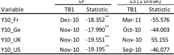
For the 1 year interest rate (variable Y1) series (Table 2), the LP tests fail to reject the null hypothesis of a unit-root at 1 percent significance level in three countries – GE, US and UK, revealing that the interest rates at 1 year of FR is stationary. The analyses of the 10 year interest rate (variable Y10) series reveal that all countries are (Table 3).
In light of these results, the cointegration hypothesis was tested with the Pi variable of the European countries against the Y1 variable of US (Table 4). The three most economically developed countries (GE, UK and US) revealed a similar pattern in the interest rate series (Y1), which could suggest a strong contagious phenomenon between them. The structural break points defined through the different
tests consistently coincide with important dates through the time-window analyzed, with special emphasis on the US.
The structural break points identified by the LS test (one break), reveal the economic impact of the September 11 2001 attacks on the US, and the repercussions in the following years with the concerted military action against Iraq.
By late 2003, the US was in the midst of the most serious world economic setback, originated by the credit boom (interest rates were at a 50-year-low and mortgage credit stood at an all-time high) and the housing bubble (prices had exceeded all previous levels).
The first half of 2004 was characterized by a trend towards gradual economic recovery. In the US, 1.2 million new jobs were created, and core inflation rose from 1.1% to 1.9%, leading the Federal Reserve to raise interest rates by 25 basis points to 1.25 %. However, the European Central Bank kept the interest rate on the main refinancing operations at 2%. The Nasdaq rose 2.22% and the Dow Jones and S&P 500 showed variations of 0.18% and 2.60%. In the Eurozone, the Paris CAC 40 and IBEX 35 went up
Variable TB1 Statistic TB1 Statistic Y1_Fr Sep‐07 ‐16.770** Sep‐07 ‐44.846 Y1_Ge Feb‐06 ‐2.048 Feb‐02 ‐4.271 Y1_UK Feb‐06 ‐2.048 Feb‐02 ‐4.271 Y1_US Feb‐06 ‐2.048 Feb‐02 ‐4.271 Note: aBoth Intercept and Trend
LS (1 break) LPa
Table 2 - Unit-root tests (variable Y1). (**) indicates critical values at 1%.
Variable TB1 Statistic TB1 Statistic Y10_Fr Dec‐10 ‐18.352** Mar‐11 ‐55.576 Y10_Ge Nov‐10 ‐17.990** Oct‐10 ‐44.003 Y10_UK Nov‐10 ‐19.551** Nov‐10 55.155 Y10_US Nov‐10 ‐19.195** Sep‐10 ‐46.077 Note: aBoth Intercept and Trend
LS (1 break) LPa
Table 3 - Unit-root tests (variable Y10). (**) indicates critical values at 1%.
4.92% and 4.41%, while the DAX in Frankfurt rose 2.64%.
During 2005, major equity markets continued their upward trend and the longer term interest rates declined. As a result of concerns about the potential inflationary consequences of the ample liquidity supply and possible lagged effects of the sharp rise in energy prices on price and wage setting, the ECB raised interest rates by 25 basis points in early December 2005. Despite this, the monetary policy remained accommodated. This partly offset the easing of overall monetary conditions due to the weakening of the euro; the ECB had taken this step in an attempt to bring short-term rates to a neutral position, as the United States Federal Reserve had done since July 2004.
Meanwhile, when the downturn in housing prices finally began in 2006, everyone had difficult in repaying their mortgages as home equity loans shrank. Subprime borrowers were, by definition, more prone to default on their mortgages than the average person. In addition, they were more likely to be poor and unemployed so had painfully few alternatives to defaulting. The tendency of increasing prices (to enable increased subprime lending) was another dangerous feedback loop of the housing bubble. As housing prices rose, banks became more inclined to increase subprime lending, which in turn spurred greater housing demand, thereby accelerating the price increase. While such cycles seemed to enable the bubble to inflate itself, they still depended on adherence to the irrational belief that housing prices would rise indefinitely. Bankers who allowed rising prices to overshadow the risks of subprime lending did so in this belief. Mimicking and reinforcing homebuyers’ representativeness heuristic (i.e. the belief that recent trends would continue unabated), the behavior of such bankers further challenges the assumed rationality of key economic actors.
Having plateaued in 2006, housing prices in 2007 stood on the edge of a precipice. They plummeted from the second quarter of that year until the first quarter of 2009, and fell 5% every three months i.e. faster than they had climbed. Housing prices continued to decline more gradually after 2009, sinking steadily through 2012 when they approached the pre-bubble, century-long average.
By 2008, developments took a turn for the worse, and the growth slowdown became acuter. In early 2009, the conclusion was that this would be a deeper
recession than the average of “Big Five” (those in Spain, 1977; Norway, 1987; Finland, 1991; Sweden, 1991 and Japan, 1992). The conjuncture of elements is illustrative of the two channels of contagion: cross-linkages and common shocks.
For instance, German and Japanese financial institutions sought more attractive returns in the US subprime market. Due to the fact that profit opportunities in domestic real estate were limited at best and dismal at worst. Indeed, in hindsight, it became evident that many financial institutions outside the US had considerable exposure to the US subprime market. Similarly, the governments of emerging markets had experienced stress, although of mid-2009 sovereign credit spreads had narrowed substantially in the wake of massive support from rich countries for the IMF fund. European banks began to face liquidity problems after August 2007, and German banks continued to lend heavily to peripheral borrowers in the mistaken belief that peripheral countries were a safe outlet. Net exposure rose substantially in 2008. Speculators focused on Greek public debt on account of the country’s large and entrenched current account deficit as well as because of the small size of the market in Greek public bonds. Greece was potentially the start of speculative attacks on other peripheral countries – and even on countries beyond the Eurozone, such as the UK – that faced expanding public debt.
By August 2011 a sharp drop in stock prices took place in markets across the US, Middle East, Europe and Asia, essentially due to fears of contagion of the European sovereign debt crisis to Spain and Italy, as well as concerns over France's current AAA rating, as well as slow economic growth in the United States and the downgrading of its credit rating. Severe volatility of stock market indexes continued for the rest of the year. In April, the S&P rating agency lowered the US credit rating to ‘negative’ from ‘stable’. Most developments in global financial markets between early September and the beginning of December were driven by news on the euro area sovereign debt crisis. In the midst of evaluation downgrades and political uncertainty, market participants demanded higher yields on Italian and Spanish -government debt. Meanwhile, difficulties in meeting fiscal targets in a recessionary environment weighed on prices for Greek and Portuguese sovereign bonds.
The contagion phenomenon quite evident in the results; reveal that the US/UK/GE trio are often the “head” of the problem followed by the remaining emergent markets (IR, FR, SP, PT and IT).
The cointegration hypothesis was tested by performing the relationship between the stock market prices and interest rates (Table 4). Bivariate cointegration was considered for this purpose, allowing for structural break tests between the price indexes of each European stock market and the interest rate at 1 year of USmarket benchmark.
(US). This test detects regime-shift as well as stable cointegration relationships. Thus, the rejection of the null hypothesis does not entangle the instability of the cointegration relationship. The differentiation of these situations is made using stationarity tests and with the structural breaks previously presented. It is possible to infer the US influence on the European equity markets through the timing of structural breaks (Tables 1 to 3) and because both variables show prolonged upward and downward movements (resumed in Table 4). An examination of the crisis reveals that economies are already quite integrated, and this resulted in its spread from the US to the rest of the world.
References
[1] Andreou, E., Ghysels, E., 2006. Monitoring disruptions in financial markets. Journal of
Econometrics, 135(1–2), 77-124.
[2] Andreou, E., Ghysels, E., Kourtellos, A., 2009.
Should macroeconomic forecasters look at daily financial data? University of North Carolina.
Mimeo.
[3] Andreou, E., Ghysels, E., Kourtellos, A., 2010. Regression models with mixed sampling frequencies. Journal of Econometrics, 158(2), 246-261.
[4] Arghyrou, M.G., 2007. The price effects of joining the Euro: Modeling the Greek experience using non-linear price-adjustment models.
Applied Economics, 39(4), 493-503.
[5] Bai, J., Perron, P., 1998. Estimating and testing linear models with multiple structural changes.
Econometrica, 66, 47-78.
[6] Bai, J., Perron, P., 2003a. Computation and analysis of multiple structural change models.
Journal of Applied Econometrics, 18, 1-22.
[7] Bai, J., Perron, P., 2003b. Critical values for multiple structural change tests. Econometrics
Journal, 6, 72-78.
[8] Bai, J., Perron, P., 2006. Multiple Structural
Change Models: A Simulation Analysis in
Econometric Theory and Practice: Frontiers of Analysis and Applied Research, D. Corbea, S. Durlauf and B. E. Hansen (eds.), Cambridge University Press, 212-237.
[9] Banerjee, A., Lumsdaine, R.L., Stock, J.H., 1992. Recursive and Sequential Tests of the Unit Root and Trend-Break Hypothesis: Theory and International Evidence. Journal of Business and
Economic Statistics, 10, 271-287.
[10] Baker, M., Nagel, S., Wurgler, J., 2007. The
Effect of Dividends on Consumption. Brookings
Papers on Economic Activity, Economic Studies Program, The Brookings Institution, 38(1), 231-292.
[11] Ben-David, D., Papell, D., 1995. Slowdowns and
Meltdowns: Post-war Growth Evidence from 74 Countries. CEPR Discussion Papers 1111.
[12] Ben-David, D., Papell, D.H., 1997. International trade and structural change. Journal of
International Economics, 43(3-4), 513-523.
[13] Ben-David, D., Lumsdaine, R.L., Papell, D.H., 2003. Unit roots, postwar slowdowns and long-run growth: Evidence from two structural breaks. Empirical Economics, 28(2), 303-319.
[14] Chou, W.L., 2007. Performance of LM-type unit root tests with trend break: A bootstrap approach.
Economics Letters, 94(1), 76-82.
[15] Demez, S., Ustaoglu, M., 2012. Exchange-Rate Volatility`s Impact on Turkey`s Exports: An Empirical Analyze for 1992-2010. Procedia -
Social and Behavioral Sciences, 41, 168-176.
[16] Esteve, V., Ibáñez, M.N., Prats, M.A., 2013. The Spanish term structure of interest rates revisited: Cointegration with multiple structural breaks, 1974–2010. International Review of Economics
& Finance, 25, 24-34. Cointegration Minimum
Variables Pi (market) and 1Y (US): models T‐Statistic 1% 5%
C ‐3.244 ‐5.130 ‐4.610 CT ‐3.515 ‐5.450 ‐4.990 CS ‐3.410 ‐5.470 ‐4.950 C ‐4.253 ‐5.130 ‐4.610 CT ‐4.079 ‐5.450 ‐4.990 CS ‐3.119 ‐5.470 ‐4.950 C ‐4.493 ‐5.130 ‐4.610 CT ‐3.671 ‐5.450 ‐4.990 CS ‐2.647 ‐5.470 ‐4.950 Note: the critical values from Gregory‐Hansen (1996a) Pi_Fr Pi_Ge Pi_UK Critical Values
[17] Gregory, A.W., Hansen, B.E., 1996. Tests for cointegration in models with regime and trend shifts. Oxford Bulletin of Economics and
Statistics, 58, 555-560.
[18] Ibrahim, S., 2009. East Asian Financial Integration: A Cointegration Test Allowing for Structural Break and the Role of Regional Institutions. International Journal of Economics
and Management, 3(1), 184-203.
[19] Karunaratne, N.D., 2010. The sustainability of Australia’s current account deficit – A reappraisal after the global financial crisis.
Journal of Policy Modeling, 32, 81-97.
[20] Kumar, A., Lee, C.M.C., 2006. Retail Investor Sentiment and Return Comovements. The
Journal of Finance, LXI (5), 2451-2486.
[21] Kurov, A., 2010. Investor sentiment and the stock market’s reaction to monetary policy.
Journal of Banking & Finance, 34, 139-149.
[22] Lee, J., Strazicich, M.C., 2003. Minimum Lagrange multiplier unit root test with two structural breaks. The Review of Economics and
Statistics, 85(4), 1082-1089.
[23] Lee, J. and Strazicich, M.C., 2004. Minimum LM
unit root test with one structural break.
Appalachain State University, Department of Economics, Working Paper No 17.
[24] Lee, J., List, J.A., Strazicich, M.C., 2006. Non-renewable resource prices: deterministic or stochastic trends? Journal of Environmental
Economics and Management, 51(3), 354-370.
[25] Lean, H.H., Smyth, R., 2007a. Do Asian stock markets follow a random walk? Evidence from LM unit root tests with one and two structural breaks. Review of Pacific Basin Financial
Markets and Policies, 10(1), 15-31.
[26] Lean, H.H., Smyth, R., 2007b. Are Asian real exchange rates mean reverting? Evidence from univariate and panel LM unit root tests with one and two structural breaks. Applied Economics, (39), 2109-20.
[27] Lumsdaine, R.L., Papell, D.H., 1997. Multiple Trend Breaks and the Unit Root Hypothesis.
Review of Economics and Statistics, 79 (2),
212-218.
[28] Marashdeh, H., Shrestha, M.B., 2008. Efficiency in emerging markets - evidence from the Emirates securities market. European Journal of
Economics, Finance and Administrative Sciences, (12), 143-150.
[29] Narayan, P.K., Smyth, R., 2005. Electricity consumption, employment and real income in Australia: evidence from multivariate granger causality tests. Energy Policy, 33, 1109-1116. [30] Narayan, P.K., 2006. The behavior of US stock
prices: evidence from a threshold autoregressive model. Mathematics and Computers in
Simulation, 71, 103-108.
[31] Nelson, C. and Plosser, C., 1982. Trends and Random Walks in Macroeconomics Time Series: Some Evidence and Implications, Journal of
Monetary Economics, 10, 139-162.
[32] Nunes, L.C., Newbold, P., Kuan, C.M., 1997. Testing for unit roots with breaks: Evidence on the Great Crash and the unit root hypothesis reconsidered. Oxford Bulletin of Economics and
Statistics, 59(4), 435-448.
[33] Perron, P., 1989. The Great Crash, the Oil Price Shock, and the Unit Root Hypothesis.
Econometrica, 57(6), 1361-1401.
[34] Perron, P., 1990. Testing for a Unit Root in a Time Series with a Changing Mean. Journal of
Business & Economic Statistics, 8(2), 153-162.
[35] Ranganathan, T., Ananthakumar, U., 2010. Give
it a break. 30th International Symposium on
Forecasting, San Diego, USA.
[36] Rao, B.B., Kumar, T.A.S., 2010. Systems GMM estimates of the Feldstein-Horioka puzzle for the OECD countries and tests for structural breaks. Economic Modelling, 27(5), 1269-1273. [37] Zivot, E., Andrews, D.W.K., 1992. Further
Evidence on the Great Crash, Oil Price Shock and the Unit Root Hypothesis. Journal of
Business and Economic Statistics, 10, 251-270.
[38] Baker, M., Nagel, S., Wurgler, J., 2007. The Effect of Dividends on Consumption. Brookings Papers on Economic Activity, Economic Studies Program, The Brookings Institution, 38(1), 231-292.
[39] Kumar, A., Lee, C.M.C., 2006. Retail Investor Sentiment and Return Comovements. The Journal of Finance LXI (5), 2451-2486.
[40] Lumsdaine, R.L., Papell, D.H., 1997. Multiple Trend Breaks and the Unit Root Hypothesis. Review of Economics and Statistics 79 (2), 212-218.
[41] Nunes, L.C., Newbold, P., Kuan, C.M., 1997. Testing for unit roots with breaks: Evidence on the Great Crash and the unit root hypothesis reconsidered. Oxford Bulletin of Economics and Statistics 59(4), 435-448.
[42] Lee, J., Strazicich, M.C., 2003. Minimum Lagrange multiplier unit root test with two
structural breaks. The Review of Economics and Statistics 85(4), 1082-1089.
[43] Lee, J., List, J.A., Strazicich, M.C., 2006. Non-renewable resource prices: deterministic or stochastic trends? Journal of Environmental Economics and Management 51(3), 354-370. [44] Narayan, P.K., 2006. The behavior of US stock
prices: evidence from a threshold autoregressive model. Mathematics and Computers in Simulation 71, 103-108.
[45] Chou, W.L., 2007. Performance of LM-type unit root tests with trend break: A bootstrap approach. Economics Letters 94(1), 76-82.
[46] Lean, H.H., Smyth, R., 2007a. Do Asian stock markets follow a random walk? Evidence from LM unit root tests with one and two structural breaks. Review of Pacific Basin Financial Markets and Policies 10(1), 15-31.
[47] Lean, H.H., Smyth, R., 2007b. Are Asian real exchange rates mean reverting? Evidence from univariate and panel LM unit root tests with one and two structural breaks. Applied Economics (39), 2109-20.
[48] Nelson, C. and Plosser, C., 1982. Trends and Random Walks in Macroeconomics Time Series: Some Evidence and Implications, Journal of Monetary Economics 10, 139-162.
[49] Perron, P., 1989. The Great Crash, the Oil Price Shock, and the Unit Root Hypothesis. Econometrica 57(6), 1361-1401.
[50] Perron, P., 1990. Testing for a Unit Root in a Time Series with a Changing Mean. Journal of Business & Economic Statistics 8(2), 153-162. [51] Andreou, E., Ghysels, E., 2006. Monitoring
disruptions in financial markets. Journal of Econometrics 135(1–2), 77-124.
[52] Andreou, E., Ghysels, E., Kourtellos, A., 2009. Should macroeconomic forecasters look at daily financial data? University of North Carolina. Mimeo.
[53] Andreou, E., Ghysels, E., Kourtellos, A., 2010. Regression models with mixed sampling frequencies. Journal of Econometrics 158(2), 246-261.
[54] Bai, J., Perron, P., 1998. Estimating and testing linear models with multiple structural changes. Econometrica 66, 47-78.
[55] Bai, J., Perron, P., 2003a. Computation and analysis of multiple structural change models. Journal of Applied Econometrics 18, 1-22. [56] Bai, J., Perron, P., 2003b. Critical values for
multiple structural change tests. Econometrics Journal 6, 72-78.
[57] Bai, J., Perron, P., 2006. Multiple Structural Change Models: A Simulation Analysis in Econometric Theory and Practice: Frontiers of Analysis and Applied Research, D. Corbea, S. Durlauf and B. E. Hansen (eds.), Cambridge University Press, 212-237.
[58] Zivot, E., Andrews, D.W.K., 1992. Further Evidence on the Great Crash, Oil Price Shock and the Unit Root Hypothesis. Journal of Business and Economic Statistics 10, 251-270. [59] Banerjee, A., Lumsdaine, R.L., Stock, J.H.,
1992. Recursive and Sequential Tests of the Unit Root and Trend-Break Hypothesis: Theory and International Evidence. Journal of Business and Economic Statistics 10, 271-287.
[60] Gregory, A.W., Hansen, B.E., 1996. Tests for cointegration in models with regime and trend shifts. Oxford Bulletin of Economics and Statistics 58, 555-560.
[61] Ben-David, D., Papell, D.H., 1997. International trade and structural change. Journal of International Economics 43(3-4), 513-523. [62] Ben-David, D., Papell, D., 1995. Slowdowns and
Meltdowns: Post-war Growth Evidence from 74 Countries. CEPR Discussion Papers 1111. [63] Ben-David, D., Lumsdaine, R.L., Papell, D.H.,
2003. Unit roots, postwar slowdowns and long-run growth: Evidence from two structural breaks. Empirical Economics 28(2), 303-319.
[64] Marashdeh, H., Shrestha, M.B., 2008. Efficiency in emerging markets - evidence from the Emirates securities market. European Journal of Economics, Finance and Administrative Sciences (12), 143-150.
[65] Narayan, P.K., Smyth, R., 2005. Electricity consumption, employment and real income in Australia: evidence from multivariate granger causality tests. Energy Policy 33, 1109-1116. [66] Ranganathan, T., Ananthakumar, U., 2010. Give
it a break. 30th International Symposium on Forecasting, San Diego, USA.
[67] Arghyrou, M.G., 2007. The price effects of joining the Euro: Modeling the Greek experience using non-linear price-adjustment models. Applied Economics 39(4), 493-503.
[68] Lee, J. and Strazicich, M.C., 2004. Minimum LM unit root test with one structural break. Appalachain State University, Department of Economics, Working Paper No 17.
[69] Ibrahim, S., 2009. East Asian Financial Integration: A Cointegration Test Allowing for Structural Break and the Role of Regional
Institutions. International Journal of Economics and Management 3(1), 184-203.
[70] Karunaratne, N.D., 2010. The sustainability of Australia’s current account deficit – A reappraisal after the global financial crisis. Journal of Policy Modeling 32, 81-97.
[71] Rao, B.B., Kumar, T.A.S., 2010. Systems GMM estimates of the Feldstein-Horioka puzzle for the OECD countries and tests for structural breaks. Economic Modelling 27(5), 1269-1273.
[72] Demez, S., Ustaoglu, M., 2012. Exchange-Rate Volatility`s Impact on Turkey`s Exports: An Empirical Analyze for 1992-2010. Procedia - Social and Behavioral Sciences 41, 168-176. [73] Esteve, V., Ibáñez, M.N., Prats, M.A., 2013. The
Spanish term structure of interest rates revisited: Cointegration with multiple structural breaks, 1974–2010. International Review of Economics & Finance 25, 24-34.